SWAT-Based Characterization of and Control Measures for Composite Non-Point Source Pollution in Yapu Port Basin, China

Abstract

The Soil and Water Assessment Tool (SWAT) was utilized to analyze the spatiotemporal distribution patterns of composite non-point source pollution in the Yapu Port Basin, China, and to quantify the pollutant load contributions from various sources. Scenario-based simulations were designed to assess the effectiveness of different mitigation strategies, focusing on both agricultural and urban non-point source pollution control. The watershed was divided into 39 sub-watersheds and 106 hydrologic response units (HRUs). Model calibration and validation were conducted using the observed data on runoff, total phosphorus (TP), and total nitrogen (TN). The results demonstrate good model performance, with coefficients of determination (R²) ≥ 0.85 and Nash–Sutcliffe efficiencies (NSEs) ≥ 0.84, indicating its applicability to the study area. Temporally, pollutant loads exhibited a positive correlation with precipitation, with peak values observed during the annual flood season. Spatially, pollution intensity increased from upstream to downstream, with the western region of the watershed showing higher loss intensity. Pollution was predominantly concentrated in the downstream region. Based on the composite source analysis, a series of management measures were designed targeting both agricultural and urban non-point source pollution. Among individual measures, fertilizer reduction in agricultural fields and the establishment of vegetative buffer strips demonstrated the highest effectiveness. Combined management strategies significantly enhanced pollution control, with average TN and TP load reductions of 22.18% and 22.70%, respectively. The most effective scenario combined fertilizer reduction, improved urban stormwater utilization, vegetative buffer strips, and grassed swales in both farmland and orchards, resulting in TN and TP reductions of 67.2% and 56.2%, respectively.

1. Introduction

Over the past three decades, rapid socio-economic development has significantly accelerated the pace of urbanization in China [1]. It is projected that the national urbanization rate will reach 80% by 2050 [2]. However, this rapid urban expansion has been accompanied by a series of environmental pollution issues, including water, air, and soil pollution [3]. Among these, water environment security has become a critical and strategic concern that constrains both urban and rural development [4]. Urbanization profoundly alters land use patterns, notably by increasing the extent of impervious surfaces, which intensifies the complexity and multi-source nature of non-point source pollution [5]. Composite non-point source pollution refers to environmental contamination caused by multiple pollution sources (agricultural, urban, and industrial) interacting through various transport pathways such as surface runoff, subsurface infiltration, and atmospheric deposition [6]. This type of pollution is characterized by pronounced spatiotemporal variability, a wide range of pollutant types, and complex interactions, making it difficult to quantitatively attribute contributions from individual sources. Agricultural and urban non-point source pollution are recognized as the two principal contributors to composite pollution [7]. Agricultural non-point source pollution typically arises from the application of fertilizers and pesticides, the discharge of livestock waste, and soil erosion via surface runoff, and is generally associated with permeable land surfaces. In contrast, urban NPS pollution is primarily linked to the proliferation of impervious surfaces—such as roads and rooftops—under intensified human activity, where rainfall events generate surface runoff that directly conveys pollutants into adjacent water bodies [8,9].

Pollution source apportionment is critical for addressing the inefficiencies of current water environment management strategies. Due to the complex land use patterns and interactions among human activities and hydrological processes, the generation mechanisms of composite non-point source pollution are more intricate than those associated with singular sources. Therefore, it is inappropriate to simplify watershed-scale pollution into either solely agricultural or solely urban sources [10,11]. The complex characteristics of composite non-point source pollution render its monitoring and control particularly challenging. To enhance resource allocation efficiency, improve pollution control capacity, and reduce environmental management costs, the quantitative identification of pollution sources is essential [12]. In China, research on non-point source pollution began relatively late, and several critical aspects such as spatiotemporal distribution patterns, pollutant load estimation, and reduction strategies remain insufficiently developed. In particular, quantitative source apportionment studies are especially scarce and often overlooked. Existing studies on non-point source pollution in the Taihu Lake Basin have predominantly focused on agricultural sources, with limited attention to the composite pollution characteristics and source contribution analysis. To address these research gaps, this study focuses on the transitional region of Xueyan Town in the Taihu Lake Basin, specifically the Yapu Port Basin. The Soil and Water Assessment Tool (SWAT) is employed to simulate and analyze the spatiotemporal distribution of composite non-point source pollution, quantify source contributions, and identify key water environment issues. The objective is to support the optimization of regional pollution control strategies and provide a scientific foundation for the integrated management of agricultural–urban runoff pollution.

The SWAT model is a semi-distributed watershed model widely used at multiple watershed scales to simulate pollutant transport, hydrological assessments, land management practices, and the impacts of land use change on non-point source pollution [13]. The model has demonstrated strong applicability in studies of both urban and agricultural non-point source pollution. For urban non-point sources, efforts have focused on refining the model’s urban database and quantifying pollutant loads. For example, Tie et al. constructed an urban non-point source pollution assessment model based on field surveys and sampling, incorporating modifications to land use data and the SWAT’s urban module to achieve high-resolution simulation and pollutant load estimation for small-scale urban watersheds [14]. In contrast, agricultural non-point source studies have focused on the effects of rainfall, land use, and management practices on pollutant distribution. Ouyang et al. applied the SWAT model to assess the impact of four land use scenarios on non-point source pollution in mountainous areas of the Yangtze River Basin, demonstrating the model’s effectiveness in pollutant accounting across land use types [15]. Similarly, Tong et al. used the SWAT to quantify agricultural pollutant loads in a target area, providing support for environmental policy-making [16]. Zhang et al. established a runoff and water quality monitoring network in the Ningxia Yellow River Irrigation District, integrating the SWAT to develop a monitoring model for agricultural non-point source pollution [17]. Wang et al. applied the model to simulate nitrogen and phosphorus reduction under various scenarios and identify optimal management practices for pollution control [18]. These studies typically treat non-point source pollution as a singular pollution type within a watershed. However, in transitional zones, where agricultural and urban sources overlap, such simplification can lead to inaccuracies. Therefore, a comprehensive approach is required to capture the complexity of composite non-point source pollution. Effective control of non-point source pollution depends on accurate source identification and the development of targeted management strategies. Control measures are generally categorized into source reduction, in-process interception, and end-of-pipe remediation. In composite pollution contexts, agricultural and urban control measures are often combined to maximize pollutant load reduction [19]. The effectiveness of such measures is highly spatially heterogeneous; thus, watershed modeling is essential to assess and optimize control efforts based on local conditions.

The Yapu Port Basin, situated within the Taihu Lake Basin, serves as the study area due to the frequent application of the SWAT model in investigating watershed-scale agricultural non-point source pollution in this region. For instance, Chang et al. employed the SWAT model to quantitatively examine the spatiotemporal dynamics of agricultural non-point source pollution in the Xitiaoxi River Basin—a key tributary of the Taihu Basin—and assessed the effects of implementing both individual and combined best management practices on water quality at the watershed outlet [20]. Similarly, Yang et al. utilized the SWAT model to simulate the distribution patterns of agricultural non-point source pollutants in the Taihu Lake Basin. Their research incorporated landscape dynamic analysis and various indices to evaluate how land use changes, alongside factors such as landscape metrics, rainfall, sediment yield, slope, and soil characteristics, influence pollution levels [21]. In summary, although the SWAT model has previously been applied in the Taihu Lake Basin, most studies emphasize agricultural non-point source pollution, lacking a quantitative analysis framework capable of classifying, zoning, and phasing pollution loads under the background of rapid urbanization. Furthermore, the application of quantitative, spatially explicit methodologies for source apportionment and classification remains limited in environmental management. Therefore, this study selects the Yapu Port Basin in Xueyan Town, Taihu Lake Basin, as the study area. The SWAT model is used to simulate the spatiotemporal characteristics of composite non-point source pollution and analyze its sources in terms of pollutant composition and critical source areas. Management scenarios for both agricultural and urban pollution control are evaluated to assess their respective reduction efficiencies. The findings aim to provide scientific guidance for the future management of composite non-point source pollution in the Taihu Lake Basin.

2. Materials and Methods

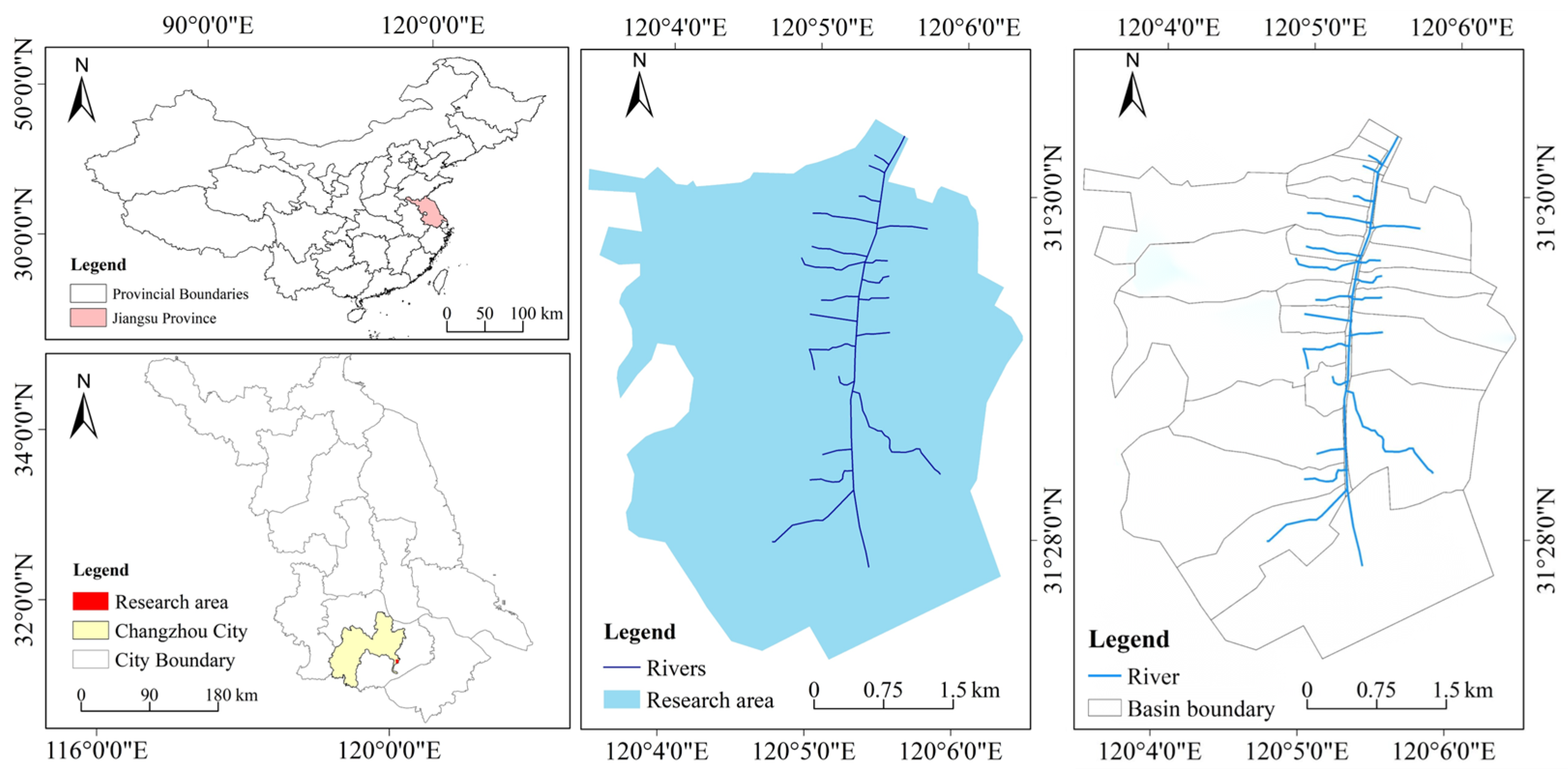
2.1. Background of the Study Area

The research site is situated in the Yapu Port Basin, Xueyan Town, Wujin District, Changzhou City, Jiangsu Province, China, spanning the latitudes 31°20′ to 31°48′ N and the longitudes 119°40′ to 120°12′ E. This area lies in the northern part of the Taihu Lake Basin, specifically within the Wujin Port Basin. It borders Mashan in Wuxi to the east and is adjacent to the Taihu Lake Basin to the south. Administratively, the region encompasses four villages: Nanshan, Yapu, Xiejia, and Taige, covering an area of 18.09 km². Within the area, there are 29 natural villages, 2618 households, a population of about 11,000, and 61 industrial enterprises. The specific geographic location of the study area is shown in Figure 1.

The study region experiences a subtropical monsoon climate, marked by four distinct seasons and plentiful sunshine. The average annual temperature is approximately 15.5 °C, with recorded extremes ranging from a high of 39.4 °C to a low of −15.5 °C. The annual average precipitation is 1068 mm, with the majority occurring during the summer and autumn months. Rainfall exhibits significant interannual variability and is unevenly distributed throughout the year. The soils in the hilly areas of the region are primarily yellow-brown soils, with a thickness ranging from 30 to 80 cm and a gravel content of 30–40%. The topsoil has a moderate humus content and medium fertility, with a slightly acidic pH of around 6.0. In the plain areas, paddy soils dominate. The topsoil tends to be acidic, while the subsoil approaches neutrality. The groundwater table is low during dry seasons, resulting in a long arable period suitable for cultivation. The physical and chemical properties of the soil are favorable for growing rice, vegetables, and fruit trees.

2.2. SWAT Model Establishment

The operation of the SWAT model depends fundamentally on two categories of input: geographic datasets and descriptive environmental parameters. Geographic data define the physical layout and spatial features of the watershed, forming the foundation for model construction. Descriptive parameters, on the other hand, provide detailed information on environmental conditions and human interventions, which the model uses to simulate key watershed processes such as runoff generation, nutrient transport, crop productivity, and soil degradation. All required inputs were collected from the relevant sources and converted into a model-compatible format, as summarized in

Table 1. Summary of input datasets used for SWAT model configuration.

	Data Type	Data Source
Spatial data	DEM	Geospatial Data Cloud
	Land use	National Cryosphere Desert Data Center
	Soil type	Institute of Soil Science, Chinese Academy of Sciences, Nanjing
Attribute data	Meteorological data	On-site automatic weather station data
	Hydrological data	Field surveys
	Physicochemical properties of soil	Harmonized World Soil Database (calculation by SPAW)

and depicted in Figure 2.

The digital elevation model (DEM), with a spatial resolution of 8 m, was obtained from the Geospatial Data Cloud platform. Land cover information, with a 30 × 30 m resolution, was sourced from the National Cryosphere Desert Data Center. The classification codes and corresponding area proportions of each land use category, as defined by the SWAT, are detailed in

Table 2. SWAT land use classification codes and their respective coverage within the watershed.

SWAT Name	Land Use Description	Proportion of Total Basin Area %
UTRN	Road	1.71%
ORCD	Orchard	21.89%
AGRL	Farmland	54.95%
URLD	Residential Area	16.42%
UNIS	Non-Built-Up Land	1.60%
WATR	Water	3.59%

.

Soil-related information was acquired from the Institute of Soil Science, Chinese Academy of Sciences, in Nanjing. Given the sparse and uneven distribution of meteorological stations across the study region, the observed climate records were incomplete. To address these data gaps, the SWAT model’s internal Weather Generator (WXGEN) was utilized to produce synthetic meteorological datasets. WXGEN serves as a robust module for generating daily weather variables—such as rainfall, air temperature, solar radiation, relative humidity, and wind speed—particularly useful when direct measurements are lacking. These climatic inputs play a critical role in simulating watershed-scale processes including evapotranspiration, crop development, and soil moisture dynamics.

The primary meteorological inputs used in this study were sourced from the Liyang weather station (elevation: 8.1 m; coordinates: 119.29° E, 31.26° N), spanning the years 2013 to 2024. The dataset comprised daily precipitation records, along with minimum and maximum temperature data. To compensate for incomplete observations, the available data were merged with WXGEN-generated outputs. The final climate data were formatted into daily time step .txt files, conforming to SWAT input requirements.

2.3. The Parameter Sensitivity of the SWAT Model

Sensitivity analysis was conducted using the Sequential Uncertainty Fitting (SUFI-2) algorithm within the SWAT-CUP (version 5.1.6) interface. A global sensitivity approach was adopted, wherein greater absolute values of the t-statistic reflect stronger parameter sensitivity, and p-values approaching zero indicate statistical significance.

2.4. Rating and Validation

Model performance was assessed using three key indicators: relative error (RE), coefficient of determination (R²), and the Nash–Sutcliffe Efficiency (NSE). In general, simulations are considered acceptable if R² exceeds 0.6, NSE is greater than 0.5, and RE falls within ±25%. The performance classification standards for these indices are summarized in

Table 3. Classification of Model Performance Evaluation Criteria.

Performance Rating	RE (%)	R2	NSE
Very Good	−10 ≤ RE ≤ +10	0.95 ≤ R2 ≤ 1.00	0.75 < NSE ≤ 1.00
Good	±10 < RE≤ ±15	0.8 < R2 < 0.95	0.65 < NSE ≤ 0.75
Satisfactory	±15 < RE ≤ ±25	0.6 < R2 ≤ 0.8	0.5 < NSE ≤ 0.65
Unsatisfactory	RE > 25 or RE < −25	R2 ≤ 0.6	NSE ≤ 0.50

[22,23].

3. Results and Analysis

3.1. Division of Sub-Basins and HRUs

The study area is located in a plain with minimal elevation variation; the DEM-based watershed delineation results can significantly deviate from actual river flow directions. To address this, a combined approach using the Burn-in algorithm and pre-defined sub-basin boundaries was adopted for improved sub-basin delineation. Specifically, the DEM was first imported, and the actual river network vector data were incorporated using the Burn-in function to assist in delineating each sub-basin. The resulting sub-basins and stream network files were then merged in ArcGIS, followed by importing the predefined watershed and river network data through the pre-defined function in SWAT. This process allowed for the accurate assignment of real sub-basin attributes based on extracted river network characteristics.

Finally, threshold values for land use, soil type, and slope were set to define the HRUs, with each HRU maintaining uniform vegetation, soil, and slope characteristics. As a result, the study area was divided into 39 sub-basins and 106 HRUs. The spatial distribution is shown in Figure 1.

3.2. The Calibration and Validation of the SWAT Model

3.2.1. Results of Runoff Calibration and Validation

The SUFI-2 algorithm in the SWAT-CUP (version 5.1.6) software was used to perform a global sensitivity analysis on the aforementioned runoff parameters, with the number of iterations set to 500. In the global sensitivity analysis, a larger P-value indicates lower parameter sensitivity, while a higher absolute value of t-Stat indicates greater sensitivity. According to the relevant literature on SWAT runoff simulation, parameters with a P-value less than 0.4 and an absolute t-Stat value greater than 1 are considered to be highly sensitive. After the iterative computations, a total of 12 highly sensitive parameters were selected for subsequent model calibration and validation, as shown in Supplementary Table S1.

In this study, the SWAT model was calibrated and validated using the monthly observed runoff data from January 2022 to December 2024 at the Yapu Port Bridge section monitoring point in Xueyan Town. The calibration period was set from 2022 to 2023, and the validation period from January 2024 to December 2024. The comparison between the simulated and observed runoff during both periods is shown in Figure 3. The model performance metrics for runoff simulation during the calibration and validation periods are presented in

Table 4. Model evaluation results for runoff calibration and validation periods.

Simulation Period	Date	NSE	R2	Re
Calibration Period	2022–2023	0.86	0.87	6.33%
Validation Period	2024	0.85	0.86	5.43%

. During the calibration period, the runoff simulation yielded Re = 6.33%, R² = 0.87, and NSE = 0.86. For the validation period, the results were Re = 5.43%, R² = 0.86, and NSE = 0.85, indicating that the model performed well during both the calibration and validation phases.

3.2.2. Results of TP and TN Calibration and Validation

A similar approach to that used for runoff parameters was applied to calibrate and validate the water quality parameters. Based on a review of the relevant literature and the model user manual, 21 parameters from the water quality module were initially selected. After iterative computation and sensitivity analysis, 12 parameters with high sensitivity were identified. These parameters significantly affect the model’s accuracy and simulation performance, and therefore require focused adjustment and optimization during the subsequent calibration process. Detailed information on the highly sensitive parameters is presented in Supplementary Table S1.

In this study, based on monthly monitoring data on TN and TP concentrations from the Yapu Port Bridge section in Xueyan Town from January 2022 to December 2024, twelve highly sensitive water quality parameters were calibrated through multiple iterations. The calibration period was set from 2022 to 2023, and the validation period from January 2024 to December 2024. The SUFI-2 algorithm in the SWAT-CUP software was used to perform multiple simulations, with 500 iterations per run. All parameters were adjusted within the recommended value ranges provided by the software. After repeated simulations, the parameter values that yielded the best performance were retained as the calibrated values for the water quality module.

The comparison of simulated and observed TN and TP loadings during the calibration and validation periods is shown in Figure 4. Model performance evaluation results for both periods are presented in

Table 5. Model evaluation results for TP and TN calibration and validation periods.

	Simulation Period	Date	NSE	R2	Re
TP	Calibration Period	2022–2023	0.85	0.86	6.97%
	Validation Period	2024	0.84	0.85	1.57%
TN	Calibration Period	2022–2023	0.87	0.89	6.01%
	Validation Period	2024	0.85	0.88	2.83%

. During the calibration period, TN simulation yielded Re = 6.01%, R² = 0.89, and NSE = 0.87, while in the validation period, the results were Re = 2.83%, R² = 0.88, and NSE = 0.85. For TP, the calibration results were Re = 6.97%, R² = 0.86, and NSE = 0.85, while the validation results were Re = 1.57%, R² = 0.85, and NSE = 0.84. These results indicate that the model performs satisfactorily for water quality simulation.

3.3. Temporal and Spatial Distribution Patterns of Composite Non-Point Source Pollution

Based on the calibration and validation of runoff and water quality parameters within the Yapu Port Basin, the model achieved satisfactory performance during both the calibration and validation periods, demonstrating strong reliability and applicability. The simulation outcomes also reflected a reasonable degree of representativeness. These results confirm that the model is well-suited for hydrological and water quality simulations in the Yapu Port Basin, offering dependable technical support for further studies in this region.

3.3.1. Temporal Distribution Patterns

• Selection of Representative Years

This study selected representative hydrological years based on the Pearson Type III distribution of annual rainfall in the Yap Port watershed from 2013 to 2024. Specifically, the years 2020, 2013, and 2021 correspond to high-flow (1433.5 mm, 20% assurance), average-flow (1229.36 mm, 50% assurance), and low-flow (1036.24 mm, 90% assurance) conditions, respectively. These years were used to analyze temporal variations in non-point source pollution.

2.

Inter-Annual Variation in Composite Non-Point Source Pollution Loads

The load of composite non-point source pollutants is influenced by multiple factors, including soil type, land use patterns, topography, and human activities. Given the short study period (2013–2021), it was assumed that no significant changes occurred in terrain, soil properties, or land use patterns within the watershed. Thus, rainfall was considered the primary factor affecting nitrogen (N) and phosphorus (P) pollutant loads across different years. As shown in Figure 5, rainfall impacts runoff volume, which serves as the main driver for nitrogen and phosphorus loads. During the study period, there were notable inter-annual variations: TN and TP loads were highest in the high-flow year (2020) and lowest in the low-flow year (2021). This indicates that rainfall exerts a decisive influence on nitrogen and phosphorus loss. According to the model outputs, rainfall significantly affects pollutant transport in the Yapu Port Basin, as nitrogen and phosphorus pollutants are mainly conveyed into water bodies via surface runoff. Increased precipitation results in greater runoff, thereby intensifying nitrogen and phosphorus losses.

3.

Intra-Annual Variation in Composite Non-Point Source Pollution Loads

Monthly TN and TP loads were extracted from the SWAT model’s output files for further analysis. Figure 6a,b illustrate the intra-annual variations for the high-flow year (2020). The results show that TN and TP loads were unevenly distributed across months, mainly concentrating during the rainy season (June–September), and fluctuated with changes in runoff, showing an initial increase followed by a decline. The TN loads peaked in July, coinciding with heavy rainfall events (319.40 mm and 475.55 mm, respectively), matching the watershed’s rainy season pattern. Similarly, the TP loads exhibited a pattern similar to that of TN, with peaks occurring in June and July. Monthly averages of TN and TP loads showed strong positive correlations with monthly rainfall; during months with low precipitation, non-point source pollution levels were minimal.

In the low-flow year (2021), Figure 6c,d shows the corresponding TN and TP loads. Although the overall pollution loads were significantly lower compared to the high-flow year, the intra-annual pattern remained similar, with the highest values occurring in the middle of the year and lowest at the beginning and end of the year. Notably, while TN and TP loads peaked in July, the runoff volume peaked in June, indicating a slight lag between peak runoff and peak pollutant loads. In months with runoff volumes below 1 m³/s, TN and TP loads accounted for less than 5% of the annual total, whereas rainy season runoff contributed approximately 48.8% of the annual load. The annual TN and TP loads were 32.4 tons and 6.6 tons, respectively, with nitrogen loads being approximately four times greater than phosphorus loads.

Figure 6e,f present the results in the average-flow year (2013). The intra-annual variation in TN and TP loads was consistent with that of the high-flow and low-flow years, with pollutant loads concentrated during the rainy season (June–September). Although the correlations with rainfall were slightly weaker compared to the high-flow year, rainfall remained the dominant factor influencing non-point source pollution. Annual TN and TP loads in the average-flow year (36.5 tons and 9.9 tons, respectively) were intermediate between those of the high- and low-flow years.

3.3.2. Spatial Distribution Patterns of Composite Non-Point Source Pollution

4.

Spatial Distribution of Nitrogen Loads in Typical Years

Figure 7c shows the spatial distribution of nitrogen loads in the low-flow year (2021). Nitrogen load intensity ranged from 0.88 to 2.78 kg/ha, with significant variation across sub-watersheds. The most heavily impacted sub-watersheds (Nos. 37, 38, and 39) were located downstream. Overall, nitrogen load intensity increased from upstream to downstream, with higher losses on the western side of the watershed compared to the eastern side. The highest nitrogen loss occurred in sub-watershed 39 (2.78 kg/ha). The upstream areas have steeper slopes and experience more severe rainfall erosion; however, industrial activity and population density are low, making soil erosion and agricultural fertilization the main pollution sources. Meanwhile, the western part of the watershed is densely planted with fruit orchards, which substantially contribute to nitrogen loss due to intensive farming practices. In the low-flow year, pollution hotspots were concentrated downstream, characterized by dense population, widespread peach orchards, and significant contributions from agricultural and domestic wastewater—making these areas critical zones for pollution control.

In the high-flow year (2020), Figure 7a shows even greater spatial variability in nitrogen loss across sub-watersheds. Higher rainfall led to increased runoff and soil erosion, resulting in greater nitrogen losses. Nitrogen runoff ranged from 4.25 to 8.03 kg/ha, with peaks in sub-watersheds 34, 38, and 39, and a maximum of 8.03 kg/ha in sub-watershed 39. The highest nitrogen losses were observed in the downstream regions, especially in areas dominated by intensive fruit orchard cultivation. In the average-flow year (2013), Figure 7b indicates that nitrogen runoff intensities ranged between those of the high- and low-flow years, from 3.12 to 5.18 kg/ha. The most severely affected areas were again the downstream orchard regions, where orchards accounted for approximately 62.7% of the land use.

5.

Spatial Distribution of Phosphorus Loads in Typical Years

Figure 8c shows the spatial distribution of phosphorus runoff in the low-flow year (2021). Due to reduced rainfall and surface runoff, phosphorus runoff was the lowest among the three typical years, ranging from 0.17 to 0.47 kg/ha. The most affected sub-watersheds (Nos. 37, 38, and 39) were located downstream, with runoff intensities exceeding 0.38 kg/ha. These areas are characterized by intensive fruit orchard and grain cultivation, high fertilizer application rates, and poor drainage conditions, leading to elevated phosphorus loss. The lack of ecological buffer zones or effective runoff control measures further aggravated phosphorus discharge into water bodies.

In the high-flow year (2020), Figure 8a shows phosphorus runoff intensities ranging from 0.44 to 0.88 kg/ha, again with hotspots located in the downstream sub-watersheds (Nos. 38 and 39). Heavy rainfall during the high-flow year facilitated the mobilization of both organic and mineral-bound phosphorus into surface runoff. Moreover, the overlap of fertilization periods with the rainy season, combined with poor soil drainage and inadequate runoff control measures, exacerbated phosphorus losses. Figure 8b shows the spatial distribution of phosphorus in the average-flow year. Phosphorus runoff intensities fell between those of the high- and low-flow years (0.30 to 0.62 kg/ha). Similarly to nitrogen, phosphorus pollution was mainly concentrated in the downstream areas, particularly in sub-watersheds 38 and 39.

3.4. The Identification of Critical Source Areas for Composite Non-Point Source Pollution in the Watershed

Based on the total nitrogen (TN) and total phosphorus (TP) loss intensity data output from the SWAT model for the Yap Port watershed, the Load per Unit Area Index (LPIAI) method was employed to identify the critical source areas (CSAs) of pollution. This method uses the loss intensity of nitrogen and phosphorus per unit area as the core indicator for evaluating non-point source pollution, and applies the Natural Breaks (Jenks) classification method to categorize TN and TP loss intensities into five levels: very mild, mild, medium, heavy, and very heavy. The classification standards are shown in

Table 6. Classification Categories and Assignment Standards for Evaluation Factors.

Indicators	Assignment Standard
TN(kg/ha)	2.750–3.005	3.005–3.513	3.513–4.160	4.160–4.544	4.544–5.330
TP(kg/ha)	0.306–0.356	0.356–0.425	0.425–0.509	0.509–0.568	0.568–0.661
Loss intensity	Very mild	Mild	Medium	Heavy	Very heavy

with sub-watersheds classified as “very heavy” designated as critical source areas. For ease of analysis, the average TN and TP loss intensities per unit area during the typical hydrological year were used for evaluation. According to the classification standards, the critical source areas were delineated using ArcGIS. The identified TN and TP critical source areas in the Yap Port watershed are shown in Figure 9a,b.

Spatially, the loss intensity generally increased from upstream to downstream, with the western watershed exhibiting higher pollution loss intensities than the eastern side. The spatial variation patterns of TN and TP loss were similar, but TP loss intensity was generally lower than that of TN. From the figure, it can be observed that the spatial distribution trends of TN and TP loss intensity were consistent, with TP pollution levels being lower than TN. The areas of very heavy TN and TP loss were mainly concentrated in the downstream region. Sub-watersheds No. 37 and 38 showed the highest TN loss intensities, while sub-watersheds No. 37, 38, and 39 exhibited the highest TP loss intensities. Overall, sub-watersheds 37, 38, and 39 had the highest loss intensities for both TN and TP and were thus identified as the critical source areas for non-point source pollution control in the watershed. These sub-watersheds cover a total area of 4.21 km², accounting for 23.29% of the entire watershed area, yet contributed 36.47% and 35.72% of the total TN and TP pollution loads, respectively. The dominant land uses in these areas are farmland and orchards, with a dense population distribution.

3.5. Evaluation of Pollution Reduction Effectiveness of Control Measures

3.5.1. Evaluation of Individual BMP Effectiveness

Considering the natural features, socio-economic development, and non-point source pollution status of the Yap Port watershed, two major categories of management measures were set: agricultural non-point source pollution control measures and urban non-point source pollution control measures. The agricultural measures targeted farmland and orchards separately and included farmland fertilizer reduction, orchard fertilizer and pesticide reduction, vegetative buffer strips, and grassed waterways. The urban measures included improving urban rainwater utilization and upgrading urban wastewater treatment facilities. The specific configurations are shown in Supplementary Table S2.

• Agricultural Non-point Source Pollution Control Measures

Under the scenario of reducing farmland fertilizer application by 20%, TN and TP reduction rates across different HRUs ranged from 29.82 to 31.77% and 24.15 to 25.22%, respectively, with average reduction rates of 30.80% and 24.67%. Under the scenario of reducing orchard fertilizer application by 25%, TN and TP reduction rates ranged from 6.89 to 7.61% and 3.21 to 4.73%, respectively, with average reduction rates of 7.25% and 3.97%. With a 5 m-wide vegetative buffer strip installed, TN and TP reduction rates ranged from 26.12 to 27.41% and 28.97 to 30.01%, with average reductions of 26.77% and 29.49%, respectively. After implementing 5 m-wide grassed waterways in farmlands and orchards, TN and TP reduction rates ranged from 24.31 to 25.63% and 26.73 to 27.35%, with average reductions of 24.97% and 27.04%, respectively. Grassed waterways significantly reduced non-point source pollutants in the watershed, particularly phosphorus.

2.

Urban Non-point Source Pollution Control Measures

Urbanization increases impervious surfaces due to human activities, sediment deposition, and waste accumulation, decreasing soil infiltration and increasing non-point source pollution runoff. Increasing the pervious area helps pollutants infiltrate the soil, thus reducing runoff. According to the simulation results, reducing the urban impervious area by 20% resulted in TN and TP reduction rates across different HRUs of 12.31–13.18% and 9.81–11.45%, respectively, with average reductions of 12.75% and 10.63%. Upgrading urban wastewater treatment to improve efficiency by 30% led to TN and TP reduction rates of 1.04–2.31% and 0.91–1.07%, respectively, with average reductions of 1.68% and 0.99%. Overall, the effectiveness of single management measures in reducing TN loads from highest to lowest was: farmland fertilizer reduction > vegetative buffer strips > grassed waterways > improving urban rainwater utilization > orchard fertilizer reduction > upgrading urban wastewater treatment. For TP loads, the order from highest to lowest effectiveness was: vegetative buffer strips > grassed waterways > farmland fertilizer reduction > improving urban rainwater utilization > orchard fertilizer reduction > upgrading urban wastewater treatment. Comparative results are shown in Figure 10.

In conclusion, agricultural non-point source pollution control measures (such as farmland fertilizer reduction, vegetative buffer strips, and grassed waterways) and the urban measure of improving rainwater utilization showed the best TN and TP removal efficiencies. However, watershed non-point source pollution control should not be limited to these measures. The selection and implementation of best management practices (BMPs) must also consider cost-effectiveness, local economic development, natural conditions, and social factors to develop targeted and practical strategies. The comprehensive evaluation of management effectiveness and feasibility is crucial for selecting the optimal pollution control measures.

3.5.2. Evaluation of Combined BMP Effectiveness

In practical watershed management, relying solely on individual best management practices (BMPs) is often insufficient to meet water quality improvement goals. A combination of multiple BMPs is generally required to maximize the effectiveness of non-point source pollution control. Therefore, this study adopted an integrated approach to non-point source pollution management by selecting and combining those agricultural and urban BMPs that demonstrated superior performance in reducing total nitrogen (TN) and total phosphorus (TP) loads. The selected BMPs included fertilizer reduction in farmland, vegetative buffer strips, grassed swales in agricultural and orchard lands, and enhanced urban rainwater utilization. Based on this, four combined BMP scenarios were developed, as summarized in

Table 7. Configuration of Combined BMP Scenarios in the Yapu Port Basin.

Scenario Number	Measure Project	Parameter Adjustment
7	Farmland Fertilizer Reduction+ Vegetative Buffer Strip	Scenario Number 1+ Scenario Number 3
8	Farmland Fertilizer Reduction+ Grassed Waterway in Farmland/Orchard	Scenario Number 1+ Scenario Number 4
9	Farmland Fertilizer Reduction+ Improve Urban Rainwater Utilization+ Vegetative Buffer Strip	Scenario Number 1+ Scenario Number 3+ Scenario Number 5
10	Farmland Fertilizer Reduction+ Improve Urban Rainwater Utilization+ Vegetative Buffer Strip+ Grassed Waterway in Farmland/Orchard	Scenario Number 1+ Scenario Number 3+ Scenario Number 4+ Scenario Number 5

.

Model simulation results (Figure 11) indicated that combined BMPs were significantly more effective in reducing TN and TP loads compared to individual measures, with average increases in TN and TP reduction rates of 22.18% and 22.70%, respectively. Among the four combined scenarios, the most comprehensive one—comprising fertilizer reduction, improved urban rainwater utilization, vegetative buffer strips, and grassed swales—achieved the highest reduction rates, with TN and TP reductions reaching 57.91% and 50.42%, respectively. The reduction effectiveness of the other combinations ranked as follows: fertilizer reduction + vegetative buffer strips > fertilizer reduction + grassed swales > fertilizer reduction + improved urban rainwater utilization + vegetative buffer strips.

It is evident that combined BMPs outperform individual measures in terms of pollutant reduction efficiency. However, the improvement in effectiveness is not linearly cumulative. As the number of implemented BMPs increases, the marginal gains in TN and TP reductions tend to diminish, indicating that BMP efficiency may plateau beyond a certain threshold. This highlights the importance of optimizing BMP combinations rather than simply increasing their quantity.

4. Discussion

The results of this study indicate that variations in nitrogen (N) and phosphorus (P) pollution loads within the Yapu Port Basin are significantly influenced by hydrological year type and agricultural activities. Differences in precipitation and runoff significantly affect the spatiotemporal dynamics of N and P loads. In high-flow years, increased rainfall and runoff enhance the mobilization and transport of pollutants, resulting in substantially elevated loads. In contrast, low-flow years with reduced hydrological activity are associated with lower pollutant loads. Due to the study area’s flat topography and limited supplementary water sources, rainfall serves as the primary driver of surface runoff, which in turn governs non-point source pollutant migration. This pattern is consistent with previous findings identifying precipitation variability as a key determinant of non-point source pollution [24,25]. For example, Geng et al. reported that a 20% increase in precipitation was shown to raise TN and TP loads by 70.8% and 78.3%, respectively, while a 20% decrease reduced them by 55.3% and 57.2%. These results support our finding that higher rainfall intensifies nutrient transport and pollution load in high-flow years [26].

Previous studies have shown that during flood seasons, concentrated precipitation intensifies surface erosion and sediment transport, leading to the runoff-mediated delivery of sediment-bound N and P into river systems [27]. In this study, intra-annual analyses similarly reveal that pollutant losses peak during the rainy season (June to August), coinciding with seasonal agricultural activities such as fertilization and irrigation. These seasonal practices, combined with frequent rainfall events, accelerate nutrient mobilization and dispersion. The results underscore the combined effects of agricultural non-point source pollution and stormwater runoff on water quality, particularly under high-flow conditions when pollution load disparities become more pronounced. Consistent with our findings, Hu et al. reported that 58.5% of annual TN and 76.0% of TP losses occurred during the rainy season (July–September) [28], highlighting the co-influence of rainfall and agricultural practices.

The spatial analysis of composite non-point source pollution reveals substantial interannual variation in N and P loss intensities, modulated by hydrological year type, land use, and ecological characteristics. In high-flow years, heightened precipitation and runoff amplify soil erosion and the export of fertilizer-derived nutrients, particularly in downstream areas with frequent agricultural activity and high rainfall. In contrast, low-flow years show lower nutrient losses due to limited runoff. Farmlands and orchards are identified as the major contributors to non-point source pollution, especially during low-flow years when fertilization periods coincide with peak rainfall, resulting in pronounced nitrogen and phosphorus losses. Downstream sub-watersheds exhibit the highest loads due to a combination of intensive land use, soil erosion, and inadequate control measures. These findings are consistent with previous studies indicating a strong correlation between nutrient loads and land use, especially in agricultural regions [29]. In the downstream areas of the watershed, excessive and improperly timed fertilization in farmlands and orchards exacerbates nitrogen and phosphorus losses [30]. The absence of effective runoff management and pollutant interception further facilitates the direct discharge of agricultural pollutants into water bodies, intensifying water quality degradation. In our study, agricultural land contributed over 70% of the total TN load and 60% of the TP load during typical years, which is consistent with previous findings in similar agricultural watersheds. For instance, a study in the Nansi Lake Basin reported that cropland was the dominant source of TN, with an average contribution rate of 62.48%, and that TN accounted for more than 94% of total non-point source pollution annually. In contrast, TP mainly originated from rural domestic sewage and livestock farming, contributing 41.74% and 40.30%, respectively [31]. The study also highlighted precipitation as the most dynamic factor influencing annual variations in both TN and TP loads. These findings reinforce the key role of agricultural activities and rainfall variability in shaping nutrient pollution patterns across different watershed systems.

Although industrial discharge and domestic sewage also contribute to nutrient pollution within the watershed, their impact is relatively minor compared to agricultural sources [32]. Fertilizer reduction measures in this study led to a 30.80% decrease in TN and 24.67% in TP, compared to only 12.75% and 10.63% reductions under urban rainwater management improvements. This highlights the characteristic diffusivity and management challenges of non-point source pollution. Therefore, pollution mitigation strategies should prioritize agricultural sources, particularly in orchards and croplands [33]. The implementation of science-based fertilization practices, optimized irrigation scheduling, and improved agricultural wastewater treatment infrastructure are essential to reduce nutrient losses and protect watershed water quality.

The results of this study indicate that agricultural BMPs generally outperform urban measures. This superiority is not solely due to differences in pollution source intensity, but also closely related to the differences in intervention pathways and operational scales between the two types of measures. Agricultural practices such as fertilizer reduction, grassed swales, and vegetative buffer strips directly influence the release and transport pathways of non-point source pollutants, offering strong capabilities for interception and reduction during transport processes [34,35]. These measures are typically implemented along slopes, field margins, or drainage ditches, where they effectively intercept nitrogen and phosphorus in surface runoff and facilitate their sedimentation, adsorption, or transformation through biological, physical, and chemical processes [36,37]. As a result, they present a “low-cost, high-benefit” potential for pollution control. In contrast, urban BMPs often rely on retrofitting impervious surfaces or enhancing wastewater treatment capacity [38]. Their intervention pathways are generally longer and more vulnerable to management discontinuities or unexpected discharge events. While measures such as increased stormwater infiltration can help reduce runoff loads, the more complex processes of pollutant deposition and accumulation in urban systems often lead to less immediate and observable pollution reduction compared to agricultural practices.

Among integrated BMP scenarios, the synergistic effects among different measures further validate the importance of “systematic management” in non-point source pollution control. Source control measures (e.g., fertilizer reduction) and transport pathway interventions (e.g., buffer strips, swales) can work in tandem to reduce overall pollutant input while increasing the residence time of pollutants in soil or vegetation systems, thus promoting their stabilization or degradation. This creates a more comprehensive pollution control chain [39]. However, it is important to note that the benefits of combining measures are not infinitely additive. As management intensity increases, functional overlap or saturation may occur among some measures, leading to diminishing marginal returns for additional BMPs. This suggests that watershed management should avoid the misconception of “more is better” and instead emphasize structural complementarity and functional layering among BMPs.

Furthermore, the sustainability and regional adaptability of measures are critical factors for practical implementation. For example, fertilizer reduction may show rapid short-term benefits but could negatively impact crop yields without a supporting nutrient management system. Vegetative buffer strips, on the other hand, require sufficient land area and regular maintenance, making them more suitable for large fields or gently sloped terrains. Therefore, the selection and deployment of any BMP should be based on a comprehensive understanding of watershed pollution characteristics, land use patterns, hydrological processes, and socio-economic context, in order to develop the most effective management strategies. While this study identifies fertilizer reduction and buffer strip implementation as effective BMPs for mitigating non-point source pollution in the Yapu Port Basin, their practical application requires careful consideration of local socio-economic and land use contexts. For instance, widespread fertilizer reduction in orchard-dominated areas may face resistance from smallholder farmers who are concerned about potential yield losses and economic returns. Moreover, the establishment of buffer strips is spatially constrained by fragmented land ownership and high land use intensity in peri-urban zones. Additionally, the lack of institutional incentives and technical support for BMP adoption may further limit their effectiveness. Therefore, policy interventions should prioritize stakeholder engagement, provide financial subsidies or ecological compensation, and encourage pilot demonstrations to balance environmental goals with farmers’ livelihoods. Tailoring BMPs to local conditions is crucial to ensure their feasibility, scalability, and long-term sustainability.

5. Conclusions

This research centers on the Yapu Port Basin, aiming to explore the spatial and temporal patterns of non-point source pollution using a model-driven approach. By assessing nitrogen and phosphorus loss intensities across the watershed, critical source zones for targeted pollution management were identified. Subsequently, simulation scenarios were developed from two angles: reducing agricultural non-point source emissions and managing urban-originated diffuse pollution. The principal findings are summarized as follows:

(1)

A composite non-point source pollution model for the Yapu Port Basin was developed using data on topography, land cover, climate, and soil properties. The model was calibrated and validated with runoff and water quality observations—specifically total nitrogen (TN) and total phosphorus (TP)—from 2022 to 2024, utilizing the SWAT-CUP software. The results indicate that the coefficients of determination (R²) for runoff, TN, and TP all exceeded 0.85, and the Nash–Sutcliffe efficiency (NSE) values were above 0.84. These metrics confirm that the model reliably replicates hydrological behavior and pollutant transport processes in the basin, making it suitable for continued application in this context.

(2)

The spatial and temporal dynamics of composite non-point source pollution and its contributing sources across the watershed were comprehensively assessed. Simulations using the SWAT model showed that nitrogen and phosphorus followed closely aligned spatial and seasonal distribution trends. Both pollutants displayed marked intra-annual variability, with significantly elevated loads during the wet season (June–September) compared to the dry season. Spatial analysis revealed a gradient of increasing pollution intensity from the upper to lower watershed, with the western region experiencing greater pollutant export. The most impacted zones were located downstream, predominantly occupied by agricultural land and orchards. Critical source zones were pinpointed using a unit-area pollutant load index. Total nitrogen and phosphorus outputs were classified into five categories using the natural breaks method. Sub-watersheds 37, 38, and 39 consistently ranked among the highest contributors to TN and TP loads. Though these areas represent only 23.29% of the watershed, they accounted for 36.47% of TN and 35.72% of TP export.

(3)

The effectiveness of various pollution control strategies in reducing composite non-point source pollution was assessed through scenario analysis. Evaluation of individual control measures indicated that practices such as fertilizer reduction in agricultural fields, the establishment of vegetative buffer zones, and the implementation of grassed swales in farmland and orchards achieved relatively high pollutant removal efficiencies, with average reduction rates exceeding 20%. Conversely, upgrading urban wastewater treatment plant discharge standards yielded limited benefits, with mean reduction rates for total nitrogen and total phosphorus remaining below 2%. Combined management strategies outperformed individual measures, enhancing the average reduction efficiencies of total nitrogen and total phosphorus by 22.18% and 22.70%, respectively. Among the various scenarios evaluated, the combined implementation of agricultural fertilizer reduction, enhancement of urban rainwater utilization, vegetative buffer zones, and grassed swales in agricultural and orchard lands resulted in the most significant pollution mitigation, achieving reduction rates of 57.91% for total nitrogen and 50.42% for total phosphorus.

6. Limitations and Future Research Directions

Although the SWAT model demonstrated satisfactory performance in simulating nitrogen and phosphorus pollution loads in the study area, several limitations remain. First, the model’s accuracy relies heavily on the availability and quality of input data, particularly long-term hydrological and water quality monitoring data, which were limited in some sub-basins. Second, while SWAT is well-suited for agricultural non-point source pollution simulation, it has a relatively coarse representation of urban runoff processes and lacks detailed urban hydrology modules, which may affect the precision of urban non-point source pollution estimations. Third, the model simplifies nutrient transport and transformation processes, which may lead to under- or over-estimations under extreme rainfall or land use change scenarios. Lastly, future research should consider integrating higher-resolution land use data, improved representation of impervious surfaces, and coupling the SWAT with urban hydrology models or pollutant fate models to enhance simulation accuracy, especially in rapidly urbanizing and ecologically sensitive regions like the Taihu Lake Basin.

References

1. Yang, L.; Fu, H.; Zhong, C.; Zhou, J.; Ma, L. Human activities accelerated increase in vegetation in Northwest China over the three decades. Atmosphere 2023, 14, 1419. [Google Scholar] [CrossRef]
2. Wang, S.T.; Bai, X.M.; Zhang, X.L.; Reis, S.; Chen, D.L.; Xu, J.M.; Gu, B.J. Urbanization can benefit agricultural production with large-scale farming in China. Nat. Food 2021, 2, 183–191. [Google Scholar] [CrossRef]
3. Liang, L.W.; Wang, Z.B.; Li, J.X. The effect of urbanization on environmental pollution in rapidly developing urban agglomerations. J. Clean. Prod. 2019, 237, 117649. [Google Scholar] [CrossRef]
4. Zhang, T.; Yang, Y.H.; Ni, J.P.; Xie, D.T. Best management practices for agricultural non-point source pollution in a small watershed based on the AnnAGNPS model. Soil Use Manag. 2020, 36, 45–57. [Google Scholar] [CrossRef]
5. Wang, Z.H.; Zhang, S.; Peng, Y.R.; Wu, C.H.; Lv, Y.P.; Xiao, K.X.; Zhao, J.; Qian, G.R. Impact of rapid urbanization on the threshold effect in the relationship between impervious surfaces and water quality in shanghai, China. Environ. Pollut. 2020, 267, 115569. [Google Scholar] [CrossRef]
6. Xue, J.Y.; Wang, Q.R.; Zhang, M.H. A review of non-point source water pollution modeling for the urban-rural transitional areas of China: Research status and prospect. Sci. Total Environ. 2022, 826, 154146. [Google Scholar] [CrossRef] [PubMed]
7. Parihar, C.M.; Singh, A.K.; Jat, S.L.; Dey, A.; Nayak, H.S.; Mandal, B.N.; Saharawat, Y.S.; Jat, M.L.; Yadav, O.P. Soil quality and carbon sequestration under conservation agriculture with balanced nutrition in intensive cereal-based system. Soil Tillage Res. 2020, 202, 104653. [Google Scholar] [CrossRef]
8. Wang, M.M.; Jiang, T.H.; Mao, Y.B.; Wang, F.J.; Yu, J.; Zhu, C. Current Situation of Agricultural Non-Point Source Pollution and Its Control. Water Air Soil Pollut. 2023, 234, 104653. [Google Scholar] [CrossRef]
9. Wang, S.R.; Rao, P.Z.; Yang, D.W.; Tang, L.H. A Combination Model for Quantifying Non-Point Source Pollution Based on Land Use Type in a Typical Urbanized Area. Water 2020, 12, 729. [Google Scholar] [CrossRef]
10. Wang, H.H.; Khayatnezhad, M.; Youssefi, N. Using an optimized soil and water assessment tool by deep belief networks to evaluate the impact of land use and climate change on water resources. Concurr. Comput. Pract. Exp. 2022, 34, e6807. [Google Scholar] [CrossRef]
11. Echogdali, F.Z.; Boutaleb, S.; Taia, S.; Ouchchen, M.; Id-Belqas, M.; Kpan, R.B.; Abioui, M.; Aswathi, J.; Sajinkumar, K.S. Assessment of soil erosion risk in a semi-arid climate watershed using SWAT model: Case of Tata Basin, South-East of Morocco. Appl. Water Sci. 2022, 12, 137. [Google Scholar] [CrossRef]
12. Chen, L.; Han, L.X.; Ling, H.; Wu, J.F.; Tan, J.Y.; Chen, B.; Zhang, F.X.; Liu, Z.X.; Fan, Y.B.; Zhou, M.T.; et al. Allocating Water Environmental Capacity to Meet Water Quality Control by Considering Both Point and Non-Point Source Pollution Using a Mathematical Model: Tidal River Network Case Study. Water 2019, 11, 900. [Google Scholar] [CrossRef]
13. Wang, Y.P.; Jiang, R.G.; Xie, J.C.; Zhao, Y.; Yan, D.F.; Yang, S.Y. Soil and Water Assessment Tool (SWAT) Model: A Systemic Review. J. Coast. Res. 2019, 93, 22–30. [Google Scholar] [CrossRef]
14. Chen, T.; Sun, F.; Yang, S.; Chen, L.; Xiong, X.; Wang, Y. Load quantification and effect evaluation of urban non-point source pollution in the Guanlan river Basin based on SWAT model. Chin. J. Environ. Eng. 2020, 14, 2866–2875. [Google Scholar]
15. Ouyang, W.; Hao, F.H.; Wang, X.L.; Cheng, H.G. Nonpoint source pollution responses simulation for conversion cropland to forest in mountains by SWAT in China. Environ. Manag. 2008, 41, 79–89. [Google Scholar] [CrossRef] [PubMed]
16. Tong, S.T.Y.; Liu, A.J.; Goodrich, J.A. Assessing the water quality impacts of future land-use changes in an urbanising watershed. Civ. Eng. Environ. Syst. 2009, 26, 3–18. [Google Scholar] [CrossRef]
17. Zhang, S.; Zhang, L.L.; Meng, Q.Y.; Wang, C.C.; Ma, J.J.; Li, H.; Ma, K. Evaluating agricultural non-point source pollution with high-resolution remote sensing technology and SWAT model: A case study in Ningxia Yellow River Irrigation District, China. Ecol. Indic. 2024, 166, 112578. [Google Scholar] [CrossRef]
18. Wang, X.; Zhang, K.; Shen, X.; Shen, F.; Guo, Y.; Shen, S. Simulation of the best management practices for agricultural non-point source pollution in the Erhai Lake Basin based on SWAT model. Chin. J. Eco-Agric. 2025, 33, 240–251. [Google Scholar] [CrossRef]
19. Liu, Y.Z.; Engel, B.A.; Flanagan, D.C.; Gitau, M.W.; McMillan, S.K.; Chaubey, I. A review on effectiveness of best management practices in improving hydrology and water quality: Needs and opportunities. Sci. Total Environ. 2017, 601, 580–593. [Google Scholar] [CrossRef]
20. Chang, J.; Yu Jie, Y.J.; Wang Fei’er, W.F.; Siyuan, Z. Cost-effectiveness analysis of best management practices for non-point source pollution in watersheds: A review. J. Zhejiang Univ. (Agric. Life Sci.) 2017, 43, 137–145. [Google Scholar] [CrossRef]
21. Yang, J.L.; Zhang, R.; Zhang, Y.Y.; Wang, G. Study on change of non-point source nitrogen and phosphorus load in Taihu Lake Basin from 1980 to 2018. Chin. J. Environ. Prot. Sci. 2022, 48, 93–101. [Google Scholar] [CrossRef]
22. Moriasi, D.N.; Arnold, J.G.; van Liew, M.W.; Bingner, R.L.; Harmel, R.D.; Veith, T.L. Model evaluation guidelines for systematic quantification of accuracy in watershed simulations. Trans. ASABE 2007, 50, 885–900. [Google Scholar] [CrossRef]
23. Nash, J.E.; Sutcliffe, J.V. River flow forecasting through conceptual models part I—A discussion of principles. J. Hydrol. 1970, 10, 282–290. [Google Scholar] [CrossRef]
24. Wang, M.C.; Huang, X.J.; Dong, Y.M.; Song, Y.Y.; Wang, D.Y.; Li, L.; Qi, X.X.; Lin, N.N. Spatiotemporal drivers of agricultural non-point source pollution: A case study of the Huang-Huai-Hai Plain, China. J. Environ. Manag. 2024, 370, 122606. [Google Scholar] [CrossRef]
25. Hu, C.C.; Wu, Q.X.; Liu, G.D.; Ran, H.Y.; Guo, M.Z.; Zhu, J.P.; Zeng, J. Nitrogen and phosphorus non-point source pollution in the upper Wujiang River Karst Basin: Critical source areas identification and influencing factors. Ecol. Indic. 2025, 170, 112989. [Google Scholar] [CrossRef]
26. Geng, R.; Zhang, P.; Pang, S.; Wang, X.; Ma, W. Impact of different climate change scenarios on non-point source pollution losses in Miyun Reservoir watershed. Trans. Chin. Soc. Agric. Eng. 2015, 31, 240–249. [Google Scholar] [CrossRef]
27. Liu, X.H.; Yang, L.Y.; Liu, L.L.; Fu, W.Z.; Wu, C.H. SWAT-Based Characterization of Agricultural Area-Source Pollution in a Small Basin. Water 2025, 17, 338. [Google Scholar] [CrossRef]
28. Hu, W.H.; Li, G.Y.; Meng, G.X.; Liming, X. Evaluation of non-point source pollution load in Fenhe Irrigation District based on SWAT model. J. Hydraul. Eng. 2013, 44, 1309–1316. [Google Scholar] [CrossRef]
29. Aboelnour, M.A.; Tank, J.L.; Hamlet, A.F.; Bertassello, L.E.; Ren, D.; Bolster, D. A SWAT model depicts the impact of land use change on hydrology, nutrient, and sediment loads in a Lake Michigan watershed. Model. Earth Syst. Environ. 2025, 11, 22. [Google Scholar] [CrossRef]
30. Tian, L.; Liu, Y.J.; Ma, Y.C.; Duan, J.; Chen, F.X.; Deng, Y.S.; Zhu, H.D.; Li, Z.W. Combined role of ground cover management in altering orchard surface-subsurface erosion and associated carbon-nitrogen-phosphorus loss. Environ. Sci. Pollut. Res. 2024, 31, 5655–5667. [Google Scholar] [CrossRef]
31. Zhang, H.; Jing, Y.; Sun, X. Evolution of spatio-temporal pattern and prevention partition of TN and TP of non-point source pollution in Nansi Lake Basin. Bull Soil Water Conserv. 2018, 38, 19–26. [Google Scholar] [CrossRef]
32. Zhang, X.Q.; Chen, P.; Dai, S.N.; Han, Y.H. Analysis of non-point source nitrogen pollution in watersheds based on SWAT model. Ecol. Indic. 2022, 138, 108881. [Google Scholar] [CrossRef]
33. Chen, L.A.; Zhang, W.S.; Tan, J.Y.; Shao, X.H.; Qiu, Y.L.; Zhang, F.X.; Zhang, X. Nitrogen and Phosphorus Pollutants Removal from Rice Field Drainage with Ecological Agriculture Ditch: A Field Case. Phyton-Int. J. Exp. Bot. 2022, 91, 2827–2841. [Google Scholar] [CrossRef]
34. Wu, S.T.; Bashir, M.A.; Raza, Q.U.; Rehim, A.; Geng, Y.C.; Cao, L. Application of riparian buffer zone in agricultural non-point source pollution control—A review. Front. Sustain. Food Syst. 2023, 7, 985870. [Google Scholar] [CrossRef]
35. Line, D.E.; Jennings, G.D.; McLaughlin, R.A.; Osmond, D.L.; Harman, W.A.; Lombardo, L.A.; Tweedy, K.L.; Spooner, J. Nonpoint sources. Water Environ. Res. 1999, 71, 1054–1069. [Google Scholar] [CrossRef]
36. Xia, Y.F.; Zhang, M.; Tsang, D.C.W.; Geng, N.; Lu, D.B.; Zhu, L.F.; Igalavithana, A.D.; Dissanayake, P.D.; Rinklebe, J.; Yang, X.; et al. Recent advances in control technologies for non-point source pollution with nitrogen and phosphorous from agricultural runoff: Current practices and future prospects. Appl. Biol. Chem. 2020, 63, 8. [Google Scholar] [CrossRef]
37. Schoumans, O.F.; Chardon, W.J.; Bechmann, M.E.; Gascuel-Odoux, C.; Hofman, G.; Kronvang, B.; Rubæk, G.H.; Ulén, B.; Dorioz, J.M. Mitigation options to reduce phosphorus losses from the agricultural sector and improve surface water quality: A review. Sci. Total Environ. 2014, 468, 1255–1266. [Google Scholar] [CrossRef] [PubMed]
38. Sansalone, J.; Raje, S.; Kertesz, R.; Maccarone, K.; Seltzer, K.; Siminari, M.; Simms, P.; Wood, B. Retrofitting impervious urban infrastructure with green technology for rainfall-runoff restoration, indirect reuse and pollution load reduction. Environ. Pollut. 2013, 183, 204–212. [Google Scholar] [CrossRef]
39. Quill, L.; Ferreira, D.; Joyce, B.; Coleman, G.; Harper, C.; Martins, M.; Hodkinson, T.; Trimble, D.; Gill, L.; O’Connell, D.W. An integrated mitigation approach to diffuse agricultural water pollution—A scoping review. Front. Environ. Sci. 2024, 12, 1340565. [Google Scholar] [CrossRef]
Figure 1. Geographic location of study area.
Water 17 01759 g001
Figure 2. Spatial distribution maps of key geographic features in the study region: (a) Elevation. (b) Land use. (c) Soil type.
Water 17 01759 g002
Figure 3. Simulated and measured monthly runoff.
Water 17 01759 g003
Figure 4. Simulated and measured monthly TP and TN.
Water 17 01759 g004
Figure 5. Output loads of (a) TN and (b) TP in different years.
Water 17 01759 g005
Figure 6. Monthly nitrogen and phosphorus loads in different hydrological years. (a) Total nitrogen load in high-flow year. (b) Total phosphorus load in high-flow year. (c) Total nitrogen load in low-flow year. (d) Total phosphorus load in low-flow year. (e) Total nitrogen load in average-flow year. (f) Total phosphorus load in average-flow year.
Water 17 01759 g006
Figure 7. Spatial distribution of total nitrogen load output in different hydrological years. (a) High-flow year. (b) Average-flow year. (c) Low-flow year.
Water 17 01759 g007
Figure 8. Spatial distribution of total phosphorus load output in different hydrological years. (a) High-flow year. (b) Average-flow year. (c) Low-flow year.
Water 17 01759 g008
Figure 9. Spatial distribution of (a) TN and (b) TP loss intensity in study area.
Water 17 01759 g009
Figure 10. Average TN and TP Reduction Rates under Different Scenarios.
Water 17 01759 g010
Figure 11. Average TN and TP Reduction Rates under Different Combined Scenarios.
Water 17 01759 g011