Phosphorus Retention in Treatment Wetlands? A Field Experiment Approach: Part 2, Water Quality

Abstract

In this study, we hypothesized and tested that physical parameters (flow, transport, and water depth) have a significantly greater influence on phosphorus (P) retention in wetlands than biogeochemical factors. Specifically, we evaluated the null hypothesis (H₀), that no significant difference exists between the influence of physical and biogeochemical parameters on phosphorus retention, against the alternative hypothesis (H₁), that physical parameters are more influential. We investigated two large wetlands (stormwater treatment areas, STAs) in south Florida: STA34C2A, which is dominated by emergent aquatic vegetation (EAV), and STA2C3, which is dominated by submerged aquatic vegetation (SAV). Building on Part 1, which mapped spatial flow resistance (K) as a vegetation-type-independent proxy for hydraulic resistance, this study (Part 2) applied a novel high-frequency (hourly) data approach with time-lagged regression modeling to estimate total phosphorus (TP) outflow concentrations. The key variables included inflow TP concentration, vegetation volume, water depth, nominal hydraulic residence time (HRT), hydraulic loading rate (HLR), phosphorus loading rate (PLR), and time lag (“P-spiral”). Multi-linear regression models for each STA identified inflow TP and water depth, a controllable physical parameter, as the most significant predictors of TP outflow, while the hour of day (a temporal proxy) contributed the least. Optimal model performance occurred with lag times of 8 and 9 days, producing R² values of 0.5788 (STA34C2A) and 0.5354 (STA2C3). In STA34C2A, high TP retention was linked to shallow water depth, dense EAV, and low K values, indicating high hydraulic resistance and reduced short circuiting. In contrast, lower TP retention in STA2C3 was associated with longer flow paths, sparse SAV, and high K values, suggesting less hydraulic control despite similar nominal HRTs. These results provide empirical support for rejecting the null hypothesis (H₀) in favor of the alternative (H₁): physical parameters, especially water depth, hydraulic resistance, and inflow dynamics, consistently exert a stronger influence on P removal than biogeochemical factors such as PLR. The findings highlight the importance of optimizing flow and depth controls in wetland design and management to enhance phosphorus removal efficiency in large, constructed wetland systems.

1. Introduction

Wetlands serve as important natural and constructed buffers that mitigate phosphorus (P) transport from terrestrial to aquatic systems and are widely recognized for their role in improving water quality by acting as sinks for nutrients, particularly P, which is a leading contributor to eutrophication in aquatic ecosystems [1,2]. Phosphorus, a key nutrient driving eutrophication in freshwater environments, is retained within wetland systems through a range of biogeochemical and physical processes (Figure 1). Biogeochemical mechanisms such as sediment interactions, redox conditions, microbial activity, and vegetation uptake have been widely studied and are commonly recognized as primary drivers of P retention [3,4]. Meanwhile, physical processes, including hydraulic loading rate (HLR), hydraulic residence time (HRT), water depth, and internal flow dynamics, have received comparatively less attention, particularly at the system scale. Wetlands’ effectiveness regarding P retention rely on both biogeochemical and physical parameters, operating over various spatial and temporal scales. Understanding the interactions between these factors is crucial for predicting and enhancing P retention.

Previous studies have shown that vegetation can influence both biogeochemical and hydrodynamic processes by slowing water flow, promoting sedimentation, and altering nutrient cycling [5]. Yet, despite this dual role, most investigations have emphasized biogeochemical attributes over the physical mechanisms that directly govern water movement and solute transport. In fact, design guidelines for constructed wetlands often treat physical parameters as fixed, rather than as dynamic and manageable variables. This oversight limits the ability to optimize wetlands for maximum phosphorus retention.

The interactions between vegetation and flow were also investigated in a series of publications [6,7,8], demonstrating how vegetation resistance and P retention depends on flow type (steady vs. pulsed) and flow characteristic (e.g., laminar, turbulent, or transient).

Despite the recognized importance of biogeochemical processes, physical parameters such as HLR, HRT, flow path, and water depth are also critical to P removal. Yet, those parameters receive disproportionately less attention in the literature. Studies that do explore these variables often do so in isolation or use generalized empirical models that fail to account for their interactions or site-specific behavior [9,10,11].

In the first phase of this research [12], we demonstrated that wetland vegetation substantially alters flow patterns, creating low-velocity zones favorable for sedimentation and P retention. We introduced the parameter “wetland transmissivity” (K) to quantify vegetation-induced flow resistance, revealing how vegetation density influences residence time and, by extension, P removal performance. These findings emphasized the need to better understand and quantify how physical parameters shape retention outcomes.

We [12] also investigated how wetland vegetation influences internal flow patterns. Using hydrodynamic modeling and field measurements, we demonstrated that plant density/type and species distribution significantly alter residence time distribution and create low-velocity zones conducive to phosphorus sedimentation. This aligns with previous findings that vegetation enhances P retention by increasing particle settling and promoting conditions favorable for P sorption onto sediments [9]. Furthermore, ref. [12] introduced a surrogate parameter, “wetland transmissivity” (K), to represent vegetation resistance to water flow. Vegetation porosity remains independent of both vegetation type and flow regime [12]. High K values correspond to sparse vegetation, or open water, and are associated with lower resistance and a faster flow regime. Conversely, low K values indicate higher plant density and higher vegetation resistance, consistent with slower moving water [12]. These findings emphasized the need to better understand and quantify how physical parameters shape P retention outcomes.

In the current study (Part 2), we build on these findings by systematically evaluating how key physical drivers such as HLR, HRT, water depth, and flow path, affect P retention in a large, constructed wetland. This study utilizes high-resolution, hourly data to investigate the relationships between hydraulic processes and total phosphorus (TP) concentrations at inflow and outflow points, offering a more refined subtle understanding of the physical controls on P removal than traditional low-frequency sampling approaches.

HLR and HRT are especially important because they directly influence the contact time between water and reactive substrates, sedimentation rates, and redox conditions, all of which mediate P transformations [13,14]. Water depth, in turn, affects thermal stratification, vegetation establishment, and the spatial distribution of aerobic versus anaerobic zones, which are crucial for P cycling. However, most wetland design guidelines treat these factors as fixed inputs rather than dynamic, manageable variables.

Wetland size (aspect ratio), morphology, and flow path also impact P retention. Shallow, low-gradient wetlands promote laminar flow, enhancing P sedimentation. Channelization or deep zones may lead to short circuiting, reducing retention. Previous studies [7,9,15] have found that increasing the flow path and contact time between inflow water and wetland substrate increased total P retention. Meanwhile, ref. [7] proposed a diagram representing P retention in terms of flow per wetland’s unit width, water depth, and water slope.

This oversight of physical parameters limits the potential to optimize wetland design and operation for P removal. As ref. [5] notes, understanding how these hydrodynamic controls interact with nutrient loads is vital for enhancing treatment performance, particularly in large-scale or agricultural catchment settings.

The second phase of our research (Part 2) aims to bridge this knowledge gap by systematically evaluating the impact of physical drivers such as HLR, HRT, and water depth on P retention in a constructed wetland. We hypothesize that among these variables one or more may emerge as both highly influential and controllable through practical design or operational interventions. To test this hypothesis, we conducted extensive phosphorus concentration monitoring at both the inflow and outflow of a large wetland system over two experimental periods and varying hydrologic conditions.

This data-driven approach offers new insights into the treatment performance of constructed wetlands. The primary focus of the current research is to investigate the relationship between hydraulic processes (i.e., water transport) and phosphorus retention. A clearer understanding of this relationship can inform strategies for optimizing P removal by managing hydraulics. Particularly, how water flows through varying vegetation communities (e.g., EAV, SAV) and how those communities influence key parameters such as HRT, water depth, and subsequently the overall P removal efficiency. Our goal is to identify which physical factors are most strongly associated with P retention and to develop evidence-based recommendations for wetland design and management. By considering this, we aim to provide practitioners and researchers with a framework that balances both biogeochemical and physical considerations, advancing the performance of wetlands as sustainable nutrient removal systems.

In summary, this investigation centers on a fundamental question: can physical parameters, which are directly controllable through wetland design and operational strategies, exert a greater influence on P retention than biogeochemical factors, which are typically less flexible or more difficult to manipulate? If so, this would have major implications for wetland management and design, offering practitioners more precise tools to enhance water treatment performance.

To explore this question, we test the following hypotheses:

• Null Hypothesis (H₀): there is no significant difference between the influence of physical parameters and biogeochemical factors on phosphorus retention in wetlands.
• Alternative Hypothesis (H₁): physical parameters (flow, transport, and water depth) have a significantly greater influence on phosphorus retention in wetlands than biogeochemical factors.

By focusing on the interaction between flow dynamics and wetland structure, including (EAV and SAV), this study seeks to identify which physical variables most strongly correlate with P retention performance. Ultimately, we aim to develop evidence-based recommendations for the design and operation of treatment wetlands that integrate both hydrodynamic and ecological considerations, offering a framework for more effective nutrient management at landscape scales.

2. Materials and Methods

2.1. Experiment Locations

Two experimental sites were selected to represent contrasting vegetative regimes: the first site is dominated by submerged aquatic vegetation (SAV) at STA-2 Cell 3 (STA2C3; Figure 2A), while the second site is dominated by emergent aquatic vegetation (EAV) at STA-3/4 Cell 2A (STA34C2A; Figure 2B). Site selection was also guided by the aspect ratio of the wetland cells, a dimensionless metric describing the proportional relationship between width and length in a rectangular system. The aspect ratios of STA2C3 and STA34C2A were 0.43 and 0.78, respectively, indicating that STA2C3 was significantly more elongated (4600 m vs. 3600 m in length) compared with STA34C2A (Figure 2A,B).

STA2C3 is characterized by two vegetation types (Figure 2A). The top and the western part of Cell 3 is dominated by SAV and open water areas, while the eastern part and the western lower section are dominated by EAV. The section with the EAV is heavily vegetated and may only be accessed via helicopter. The cell interior is intercepted in the longitudinal and transverse directions by remnant agricultural canals. Most of the transverse canals are perpendicular to the southerly flow and dominated by EAV, which affected water flow. During this experiment, flow (HLR), water depths, and P concentrations at inflow and outflow were collected in STA2C3 between 30 August 2013, and 2 December 2013. A hydraulic wave experiment with a pre-determined frequency (Part 1) was conducted between 8 October 2013, and 30 October 2013.

STA34C2A is EAV dominated (Figure 2B). Flow, water depth, and P concentrations at inflow and outflow were collected between 19 May 2014, and 1 February 2015 for the P removal experiment. The hydraulic wave test with a pre-determined frequency was conducted from 4 August 2014 to 24 September 2014. Missing data were excluded from the analysis when there were no discharges at the inflow site in both cells (i.e., G333 and G377).

Water level loggers were deployed in both cells at numerous locations to monitor water surface elevations at 15 min intervals (Figure 1; [8]). Data collected by these loggers were used to determine a surrogate (K) for vegetation resistance [7,8], calculate dynamic water levels (i.e., water depth) inside the cell during the experiments [8], and determine flow type (fast or slow/plug flow type), independent of vegetation type.

2.2. Definitions of Key Variables

2.2.1. Hydraulic Loading Rate (HLR)

HLR is calculated using the following equation:

$$HLR=\mathrm{86,400}{\displaystyle \frac{\mathrm{Q}}{\mathrm{A}}}$$

(1)

where Q is surface water inflow (m³ s⁻¹), A is the effective treatment (wetted perimeter) area of the constructed wetland (m²), and HLR is the hydraulic loading rate in meter day⁻¹, and 86,400 is the number of seconds in a day.

2.2.2. Water Depth (D)

Water depth is commonly calculated as the average stage between tail (at inflow structure) and head (at outflow structure) water stages, minus the average ground elevation inside the wetland [16,17,18]. A dynamic water depth was calculated as the average of all observations from all interior stations deployed inside the wetland (e.g., 20 and 23 pressure sensors in both experiments) minus the average ground elevation. The dynamic water depth was calculated on an hourly basis from all water level loggers’ measurements. There was almost no significant difference (α < 0.05) between the two means from the two different methods, and, therefore, the average water depth for this analysis was calculated using the conventional method [(tail + head)/2 − (average cell ground elevation)].

2.2.3. Nominal Hydraulic Residence Time (HRT₁)

The treatment efficiency of a wetland depends on HRT [19,20,21,22,23,24,25]. HRT is the amount of time a parcel of water, for example, introduced through the inflow, travels through the wetland, and leaves at the outflow structures. It is hypothesized that outflow P concentration will decrease as HRT increases, yet it is not a linear relationship. As water can move at different rates and volumes through large, constructed wetlands, particularly in those heavily vegetated STAs (EAV or SAV), the “actual” or true HRT is hard to measure. Hydraulic retention time (HRT) is the average amount of time a compound/nutrient remains in a treatment wetland. In general, a nominal HRT or HRT₁ (in days) is easily calculated using a simple equation [1,26,27,28]:

$${HRT}_1={\displaystyle \frac{A·D}{Q_{out}·\mathrm{86,400}}}$$

(2)

where Q_out is the surface water outflow in m³ s⁻¹ (i.e., G334 or G377), A is the constructed wetland’s effective treatment area in m², and D is the water depth in meters. Nominal HRT₁ is commonly known as HRT and, for most STAs in south Florida, the annual average HRT₁ is approximately 2 weeks (14 days). HRT₂ is calculated by Equation (2), where A is calculated by subtracting the area occupied by vegetation from the total wetland area (wetland’s effective treatment area in m²; Figure 2). Of particular interest is the approach to correct HRT estimates based on errors introduced by ignoring plant volume (i.e., phytomass) and topographic uncertainty in estimating water volume in a heavily vegetated wetland system. Water volume projected by the novel approach, below 2 feet water depth, overestimated water volume by 60 percent, a significant impact on estimating HRT values in a heavily vegetated wetland. HRT also can be determined through conservative tracer studies, which provide a one-time value, a snapshot. Tracer studies are expensive to implement in a large, constructed wetland, designed to determine hydraulic efficiency, and areas of short circuiting [1,26,27,28].

2.3. Water Quality Sampling Method

Phosphorus concentrations (μg L⁻¹) were measured at sub-daily intervals with two remote phosphorus analyzers (RPA). The RPA combines automated sampling equipment with an automated micro-laboratory and is able to collect a considerable number of TP samples at remote locations for extended periods of time [19]. One RPA was deployed at the center structure of the inflow and outflow of each cell during the experiments. RPA sampling intervals started a few weeks prior to the start of the hydraulic field experiment, at 3-h, then 1.5-h sampling intervals during both field experiments and thereafter for 1 week, and then back to the 3-h sampling intervals. RPA data gaps existed at STA34C2A due to a power failure (lightning strikes). Linear interpolation was used to fill in small data gaps, while HEC-DSSVue (https://www.hec.usace.army.mil/software/hec-dssvue/downloads.aspx, accessed on 21 February 2025) was used to linearly interpolate those observations into hourly datasets. HEC-DSSVue is a Java-based visual utilities program that allows users to plot, tabulate, edit, and manipulate data in a HEC-DSS database file. The data were combined with discharge inflow (Q = m³ s⁻¹) and the wetland effective treatment area (A = m²) to calculate phosphorus loading rate (PLR = g m⁻² year⁻¹):

$$PLR={\displaystyle \frac{{TP}_{in}·Q·\mathrm{31,556.952} }{A}}$$

(3)

RPA data for STA2C3 covered the P experiment period from 30 August 2013, to 2 December 2013 (Figure 3); the hydraulic experiment period began on 8 October 2013, and ended on 30 October 2013 (Figure 4). Data collection during the hydraulic wave experiment was hourly as often as possible. All hydraulic and P data collected at the inflow and outflow structures for STA34C2A were reviewed for missing data. The final data analysis period extended from 20 June 2014, to 1 February 2015, and from 4 August 2014, to 24 September 2014, representing P removal and hydraulic sampling experiment periods, respectively (Figure 5 and Figure 6).

Hourly discharges and TP concentrations at inflows (G333 and G377) and outflows (G334 and G378) were used to calculate TP/mass loading (Equation (3)) and hydraulic loading rates (Equation (1)) for further data analysis. Average water depth within Cell 3 and Cell 2A, collected on an hourly basis, were obtained by subtracting average ground elevation (topographic survey in 2010) from the average stage elevations at inflow and outflow structures. All variables used in the analysis were either collected or interpolated (using HEC-DSSVue) to obtain hourly values and were combined into a single database for further analysis.

2.4. Data Analysis

A combination of descriptive statistics together with graphical techniques were employed to identify seasonality or trends, and describe relationships, if any, in the time series observations. All analyses were performed with the hourly values calculated from the original observations. Statistics were calculated with JMP (Version 12, SAS Institute Inc., Cary, NC, USA) and SigmaPlot (Version 13, SPSS, Inc. Chicago, IL, USA). The level of significance (α) was set at 0.05 for all analyses. Other techniques were used: box and whisker plots were developed and summarized (i.e., top and bottom of box = 75th and 25th percentiles, respectively, midline in box = median; ends of whiskers denote 5th and 95th percentile, respectively, solid black line = mean values). Linear and multi-linear regressions were used to assess the relationship between P concentrations at the outflow sites (G334 and G378), and other key variables such as HLR, PLR, HRT, water depth, and time of day (hour).

3. Results

3.1. Phosphorus Concentration Dynamics During Experimental Periods

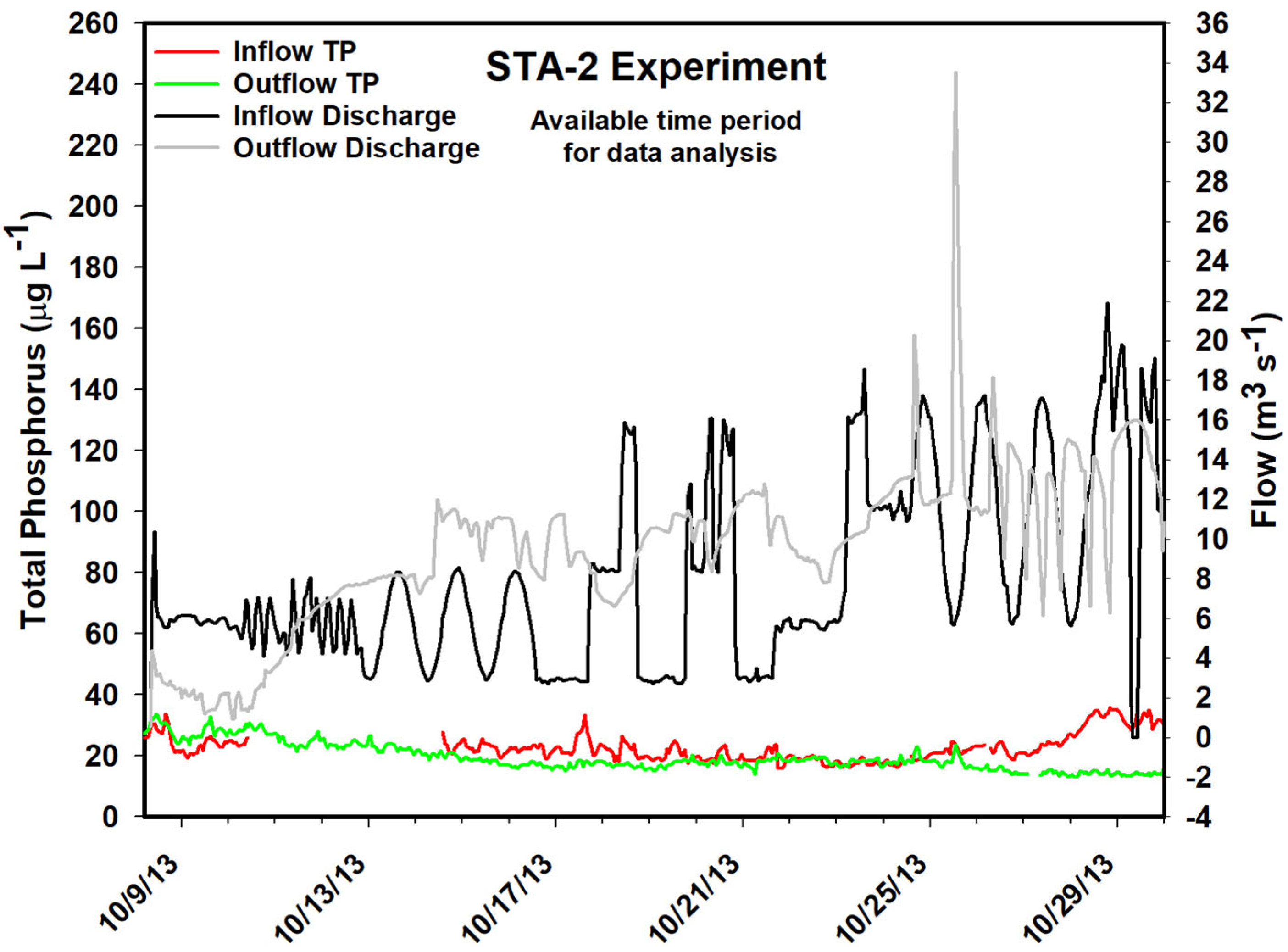
A marked discrepancy in TP concentration values was observed between the P removal experiment and the hydraulic field experiment in STA2C3, a trend not evident in STA34C2A (

Table 1. Descriptive statistics of all variables (hourly intervals) used in the analysis for the period 30 August 2013, through 2 December 2013, and during the hydraulic field test (8 October 2013, through 30 October 2013) in STA2C3.

P Removal Sampling Period: 30 August 2013, Through 2 December 2013 (STA2C3)
Variables	Size	Missing	Mean	Std. Dev	Std. Error	Range	Max	Min	Median	25%	75%
Qin (m3 s−1)	2265	0	3.53	6.40	0.14	32.45	32.45	0.00	0.00	0.00	5.56
Qout (m3 s−1)	2265	0	5.41	6.35	0.13	41.73	39.69	−2.04	3.46	0.00	8.93
TPin (µg L−1)	2265	141	47.00	34.00	0.73	216.00	231.00	15.00	34.00	24.00	60.00
TPout (µg L−1)	2265	250	20.00	4.00	0.08	26.00	38.00	12.00	20.00	18.00	23.00
Water Depth (cm)	2265	0	55.40	11.40	0.24	74.90	102.10	27.20	53.00	48.50	60.70
PLR (g/m2/yr)	2265	0	0.77	2.49	0.05	19.35	19.35	0.00	0.00	0.00	0.28
HLR (cm/day)	2265	0	3.39	6.16	0.13	31.21	31.21	0.00	0.00	0.00	5.35
HRT2 (days)	2265	0	19.90	20.50	0.40	63.0	63.20	0.10	8.50	4.30	41.2
HRT1 (days)	2265	0	27.90	22.60	0.50	65.8	70.60	4.80	14.80	9.30	50.3
Hydraulic Field Test Period Sampling Period:8 October 2013, through 30 October 2013 (STA2C3)
Qin (m3 s−1)	530	0	8.08	4.61	0.20	21.90	21.90	0.00	6.43	4.99	11.42
Qout (m3 s−1)	530	0	9.51	3.99	0.17	32.75	33.79	1.04	10.09	7.70	11.76
TPin (µg L−1)	530	104	22.78	4.59	0.22	20.50	36.50	16.00	21.88	19.34	24.41
TPout (µg L−1)	530	4	19.29	4.51	0.20	20.75	33.75	13.00	18.00	16.25	22.00
Water Depth (cm)	530	0	59.40	7.28	0.32	33.83	74.98	41.158	60.05	57.00	63.09
PLR (g/m2/yr)	530	104	0.69	0.48	0.02	2.51	2.51	0.00	0.56	0.36	0.93
HLR (cm/day)	530	0	7.77	4.43	0.19	21.06	21.06	0.00	6.18	4.80	10.98
HRT2 (days)	530	0	4.74	4.62	0.20	61.88	63.17	1.29	4.04	3.50	4.29
HRT1 (days)	530	0	13.24	18.00	0.78	64.50	69.50	5.00	6.67	5.92	9.01

and

Table 2. Descriptive statistics of all variables (hourly intervals) used in the analysis for the P removal sampling period 19 May 2014, through 1 February 2015, and during the hydraulic field experiment (4 August 2014, through 24 September 2014) in STA34C2A.

P Removal Sampling Period: 19 May 2014, Through 1 February 2015 (STA34C2A)
Variables	Size	Missing	Mean	Std. Dev	Std. Error	Range	Max	Min	Median	25%	75%
Qin (m3 s−1)	6196	0	4.96	9.36	0.12	68.41	68.41	0.00	0.00	0.00	6.23
Qout (m3 s−1)	6196	0	3.82	6.21	0.08	28.31	28.31	0.00	0.25	0.00	6.18
TPin (µg L−1)	5645	142	55.00	19.00	0.26	324.00	343.00	19.00	54.00	45.00	62.00
TPout (µg L−1)	5795	853	17.00	3.00	0.05	23.00	30.00	7.00	16.00	14.00	19.00
Water Depth (cm)	6196	0	56.08	14.32	0.18	60.31	98.27	37.96	50.23	45.78	62.22
PLR (g/m2/yr)	5129	108	1.23	2.91	0.04	38.55	38.55	0.00	0.00	0.00	1.34
HLR (cm/day)	6196	0	4.17	7.86	0.10	57.45	57.45	0.00	0.00	0.00	5.24
HRT2 (days)	6196	0	18.10	16.20	0.20	66.70	66.80	0.10	13.8	5.50	24.60
HRT1 (days)	6196	0	22.50	17.20	0.20	74.30	74.30	0.10	18.1	9.30	28.80
Hydraulic Sampling Period: 4 August 2014, through 24 September 2014 (STA34C2A)
Qin (m3 s−1)	1248	0	11.92	12.58	0.36	68.41	68.41	0.00	9.68	0.00	21.21
Qout (m3 s−1)	1248	0	7.09	7.92	0.22	28.31	28.31	0.00	3.47	0.00	15.28
TPin (µg L−1)	1248	77	57.00	11.00	0.33	82.00	108.00	26.00	55.00	49.00	62.00
TPout (µg L−1)	1248	40	16.00	3.00	0.09	20.00	27.00	7.00	16.00	14.00	18.00
Water Depth (cm)	1248	0	67.33	15.83	0.45	54.24	96.58	42.34	68.03	51.85	82.42
PLR (g/m2/yr)	1248	77	2.22	2.46	0.07	13.62	13.62	0.00	1.51	0.00	4.22
HLR (cm/day)	1248	0	10.01	10.56	0.30	57.45	57.45	0.00	8.13	0.00	17.82
HRT2 (days)	1248	0	11.00	9.50	0.30	28.00	29.60	1.50	6.50	2.50	19.20
HRT1 (days)	1248	0	15.70	10.30	0.30	29.90	34.50	4.60	12.80	5.80	24.70

). During the P removal period (30 August–2 December 2013), mean TP concentrations in STA2C3 were 47 ± 0.73 µg L⁻¹ at the inflow and 20 ± 0.08 µg L⁻¹ at the outflow. In contrast, during the hydraulic experiment period, mean TP concentrations were 23 ± 0.22 µg L⁻¹ at the inflow and 19 ± 0.20 µg L⁻¹ at the outflow (Table 1).

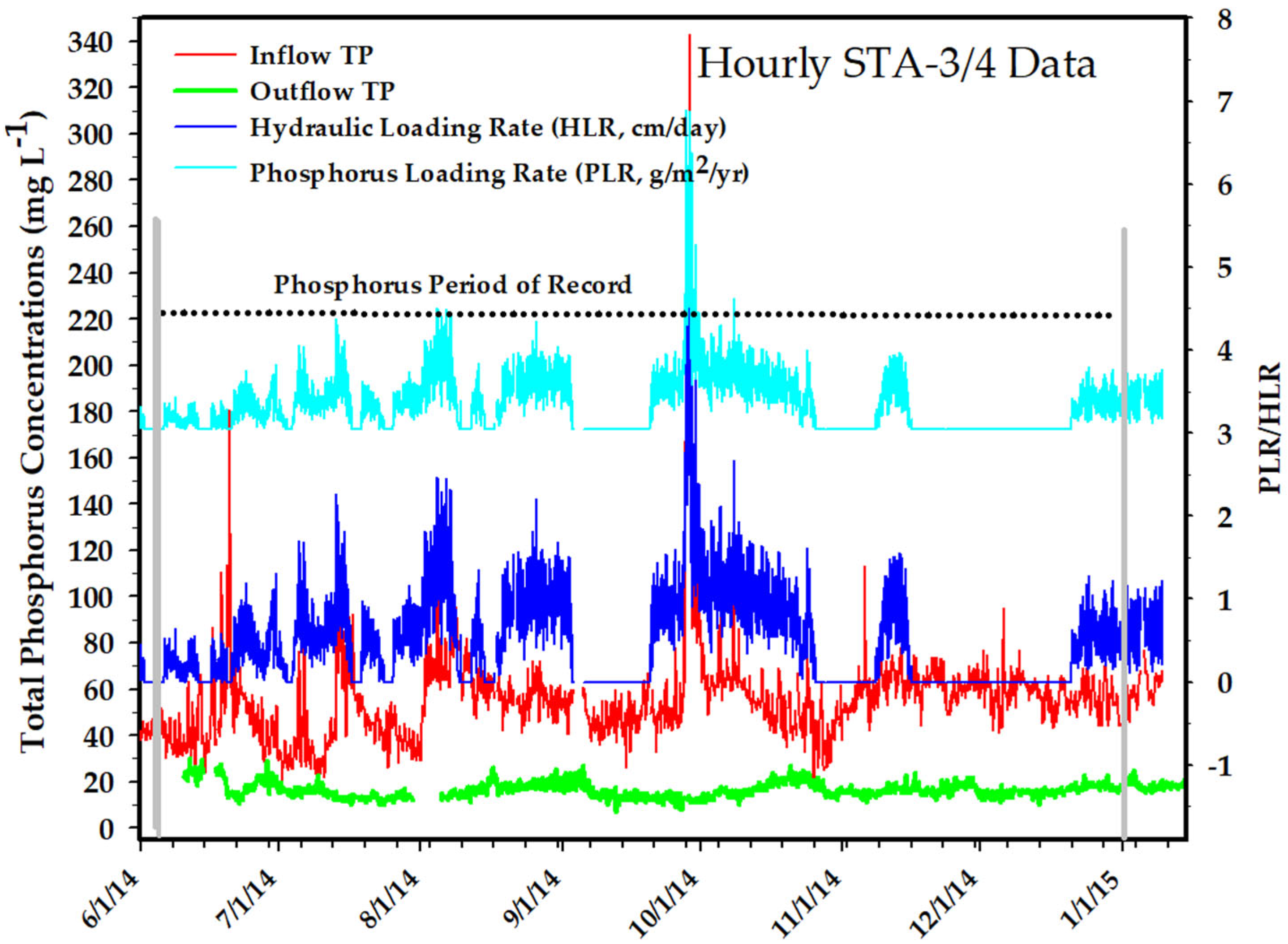
Similarly, STA34C2A exhibited consistent P concentrations across both experimental periods. During the P removal period, mean TP values were 55 ± 0.26 µg L⁻¹ at the inflow and 17 ± 0.05 µg L⁻¹ at the outflow. These values closely align with those observed during the hydraulic period, where TP concentrations averaged 57 ± 0.33 µg L⁻¹ and 16 ± 0.09 µg L⁻¹ at the inflow and outflow, respectively (Table 2).

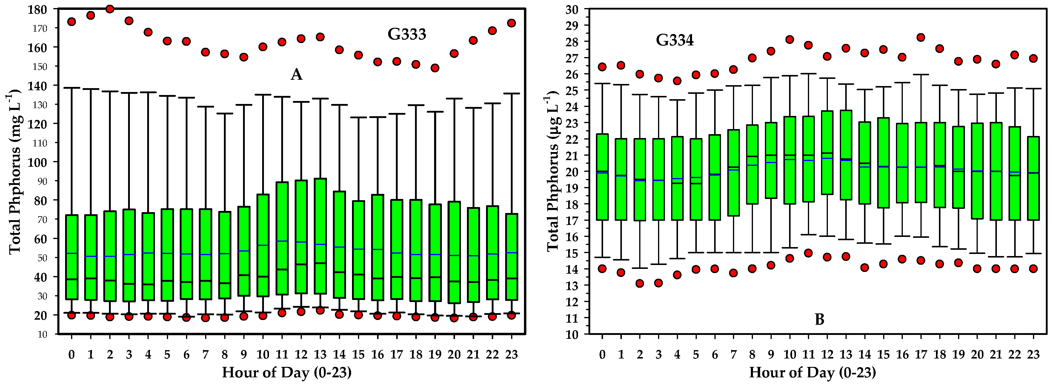
The hourly TP concentration measurements at both inflow and outflow locations revealed a consistent diel (24 h) cycle during both experimental phases (Figure 7). TP concentrations increased gradually beginning around 07:00, peaking between 12:00 and 13:00, and declining steadily to a minimum around midnight (Figure 7B). These diel trends are consistent with previous findings on nutrient cycling in wetland systems [20].

The statistical analysis confirmed significant differences in TP concentrations between diurnal (daytime) and nocturnal (nighttime) periods (p = 0.05), with this pattern being more pronounced at the outflow sites (Figure 7B). Paired t-tests for STA2C3 further indicated statistically significant differences between the concentrations measured at 10:00 and 23:00 at both inflow and outflow locations (α = 0.02). In contrast, for STA34C2A, this time-based difference was significant only at the outflow site (G378; α = 0.025), with no corresponding significance observed at the inflow (G377) (Figure 8A,B).

Normality testing using the Shapiro–Wilk test indicated that TP concentration data at inflow sites in both STA2C3 and STA34C2A deviated from a normal distribution, suggesting a stochastic component in P dynamics. For the STA34C2A outflow (G378), the difference in median TP values between 10:00 and 23:00 was not statistically significant (p = 0.165), indicating that observed variations may be attributed to random sampling variability. Conversely, the inflow site (G377) exhibited a statistically significant difference in median TP between the same time points (p = 0.002), pointing to a non-random, time-dependent fluctuation in TP levels.

The findings of this study highlight the critical role of physical parameters, particularly hydraulic retention time (HRT), water depth, and flow path geometry, in governing P retention in constructed wetlands. These physical factors often surpass biogeochemical processes in determining the efficiency of P removal. For instance, a study by [21] demonstrated that water residence time is a primary factor controlling P retention in small, constructed wetlands treating agricultural drainage water. Their research indicated that during high discharge events, shorter residence times led to reduced P retention, emphasizing the importance of maintaining adequate HRT for effective nutrient removal. Similarly, ref. [22] found that sediment deposition and accumulation, influenced by hydraulic load and flow dynamics, significantly affect P retention in small, constructed wetlands. Their study highlighted that high hydraulic loads can lead to increased resuspension and reduced sediment accumulation, thereby diminishing the wetland’s capacity to retain phosphorus. Moreover, a meta-analysis revealed that wetland hydrology and morphometry, including flow regulation and wetland size, are key controls of phosphorus retention [23]. The study emphasized that regulated flow regimes and appropriate wetland sizing can enhance P retention by promoting settling and uptake processes. Meanwhile, ref. [24] demonstrated that the effects of both water depth and wetland area, and also wetland water volume, may be important for N removal.

These studies collectively underscore the importance of considering physical design and operational parameters in the development and management of constructed wetlands for P removal. By optimizing factors such as HRT, water depth, and flow path geometry, it is possible to enhance the efficiency of P retention, thereby improving water quality outcomes in agricultural and wastewater treatment contexts.

3.2. Hourly Regression Results

Simple linear regression analyses did not yield statistically significant relationships between outflow TP concentrations and individual predictor variables (e.g., PLR) for either STA2C3 or STA34C2A. This outcome was consistent across both experimental periods (i.e., phosphorus removal and hydraulic field studies) and for both hourly and daily average datasets. In contrast, multiple linear regression (MLR) models provided improved explanatory power compared with univariate models (Figure 9).

In the MLR analysis, a time of day variable (“Hour”, ranging from 00 to 23) was incorporated as a predictor to account for diel variation in TP concentrations. The regression model was consistently applied to both stormwater treatment areas (STAs) using the following formulations, where Equations (4) and (5) are used for daily-averaged and hourly data:

TP_out = PLR + TP_in + water depth + HLR + HRT

(4)

TP_out = Hour + TP_in + water depth +PLR + HLR + HRT

(5)

To evaluate transport time dynamics, a time lag variable (ranging from 0 to 240 h or 0–10 days) was introduced to Equation (5). This lag represents the estimated travel time for P from inflow to outflow, encompassing HRT, biogeochemical spiraling, and short circuiting within the wetland system. When the lag variable was included, HRT was excluded from the regression model to avoid multicollinearity.

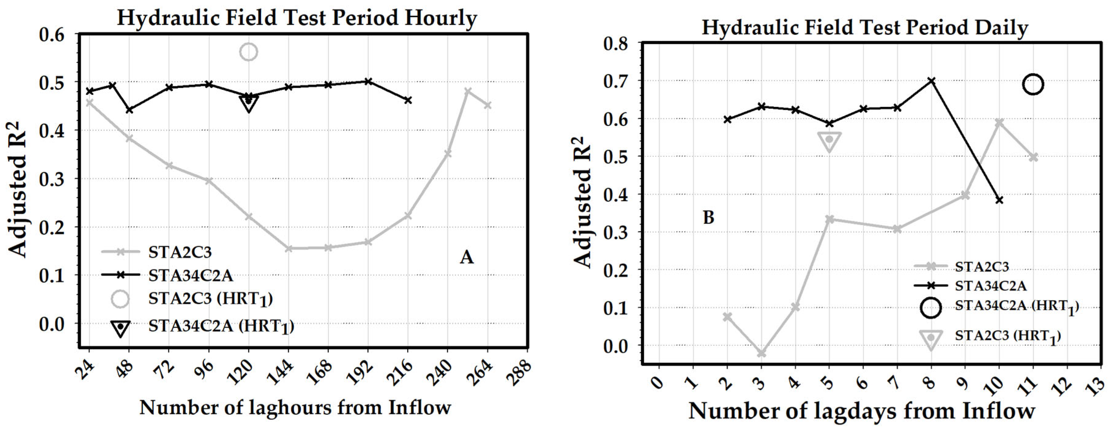
During the hydraulic sampling period, the MLR model incorporating a 0-h lag produced adjusted R² values of 0.5616 (0.5834 with HRT₁) for STA2C3 and 0.4558 (0.5554 with HRT₁) for STA34C2A (Figure 9A). This indicates an improved model fit when nominal HRT (HRT₁) was used compared with the empirically adjusted HRT₂.

In STA2C3, the most influential predictors were water depth, hydraulic loading rate (HLR), PLR, inflow TP concentration, and HRT₂ (all p << 0.01), with the hour of day variable being the least significant. Substituting HRT₁ for HRT₂ yielded a similar ranking, with water depth remaining the most influential variable and hour, again, being the least significant.

Conversely, in STA34C2A, inflow TP concentration emerged as the most significant predictor, followed by HRT₂, water depth, PLR, and hour (p << 0.01), with HLR being the least significant. When HRT₁ was used in place of HRT₂, the order shifted slightly: HRT₁ > water depth > inflow TP > PLR > hour (p < 0.01), with HLR remaining the least significant.

When the lag variable replaced HRT in the model, the highest adjusted R² values indicated optimal lags of 216 h (9 days) for STA2C3 and 192 h (8 days) for STA34C2A during the hydraulic period (Figure 9A). These values are within range but slightly lower than the nominal HRT estimates derived from field data, which were 16 days (384 h) for STA2C3 and 13 days (312 h) for STA34C2A using HRT₁, and 11 days (264 h) and 5 days (120 h), respectively, using HRT₂ (Figure 9B).

Notably, the inclusion or exclusion of the hour of day variable did not significantly affect the adjusted R² values in either STA, suggesting that diel variability, while present, contributes minimally to the overall variability in outflow TP concentrations at this scale.

Finally, the higher adjusted R² values obtained using HRT₁ rather than HRT₂ suggest potential inaccuracies in the empirical adjustments applied to derive HRT₂, which accounts for vegetative volume and topographic irregularities. These discrepancies highlight the importance of accurate site-specific hydrological characterization for the predictive modeling of phosphorus dynamics in treatment wetlands.

The multiple-linear regression model results improved using HRT₁ (i.e., nominal HRT) compared with HRT₂ for STA2C3 and STA34C2A, respectively, during the hydraulic sampling period. The noted increase in adjusted R² when HRT₁ was included in the place of HRT₂ suggests that the error model used to account for the volume of vegetation and topographic irregularities in the study site to calculate HRT₂ is inaccurate (Figure 9B).

3.3. Daily Regression Results

During the hydraulic sampling period (8–30 October 2013), the daily mean TP concentrations in STA2C3 were 23 ± 1.28 μg L⁻¹ at the inflow and 19 ± 4.43 μg L⁻¹ at the outflow (

Table 3. Descriptive statistics of all variables (daily intervals) used in the analysis during the hydraulic field experiment (8 October 2013, through 30 October 2013) in STA2C3 for the period 5 August 2014, through 24 September 2014 (for STA34C2A).

Variables (STA2C3)	Size	Missing	Mean	Std. Dev.	Std. Error	Range	Max	Min	Median	25%	75%
TPin	23	4	23.60	5.59	1.28	20.88	38.50	17.63	22.25	19.63	25.25
TPout	23	0	18.99	4.43	0.92	14.25	27.88	13.63	17.38	16.13	21.25
Water Depth (cm)	23	0	60.50	8.25	1.72	34.70	77.10	42.40	60.70	57.30	63.70
PLR	23	4	0.69	0.53	0.12	2.32	2.32	0.00	0.59	0.37	0.76
HLR	23	0	7.20	4.51	0.94	17.53	17.53	0.00	5.78	4.06	9.00
HRT1	23	0	15.60	21.33	4.45	65.13	70.38	5.25	6.71	5.83	9.79
Variables (STA34C2A)	Size	Missing	Mean	Std. Dev	Std. Error	Range	Max	Min	Median	25%	75%
TPin (µg L−1)	52	1	56.63	9.80	1.37	44.76	87.54	42.78	55.58	49.63	60.85
TPout (µg L−1)	51	0	16.28	2.70	0.38	10.64	22.79	12.15	16.07	13.78	18.64
Water Depth (cm)	52	0	67.33	15.88	2.20	52.15	95.07	42.91	67.59	51.05	82.20
PLR (g/m2/yr)	52	1	2.17	2.15	0.30	7.91	7.91	0.00	1.61	0.00	4.30
HLR (cm/day)	52	0	10.01	9.32	1.29	33.91	33.91	0.00	8.89	0.00	17.91
HRT1 (days)	52	0	15.73	10.42	1.45	29.55	34.43	4.88	12.79	5.79	25.00

). In STA34C2A, the corresponding values were 56 ± 1.37 μg L⁻¹ at the inflow and 16 ± 0.38 μg L⁻¹ at the outflow (Table 3). Although inflow TP concentrations exhibited greater variability in STA2C3 compared with STA34C2A (nearly twice the range), the mean and median TP values within each STA were nearly identical, indicating a relatively symmetrical distribution of daily TP measurements.

Multiple linear regression (MLR) models incorporating lag times (i.e., from 1 to 10 days) were applied to assess the delayed response of outflow TP concentrations (TP_out) to changes in inflow concentrations (TP_in), alongside other key hydraulic and biogeochemical variables (Figure 9B). For STA2C3, the strongest model performance was observed with a 10-day lag, yielding an adjusted R² of 0.5889. In this model, TP_in was the most influential predictor (p = 0.056), followed by hydraulic loading rate (HLR), phosphorus loading rate (PLR), and water depth.

A parallel analysis using hydraulic residence time (HRT) instead of lag days showed that models incorporating nominal HRT (HRT₁) outperformed those using empirically adjusted HRT (HRT₂). Specifically, a model with a zero-day lag and HRT₁ yielded an adjusted R² of 0.5562, compared with 0.5440 when HRT₂ was used. Field-based estimates of mean HRT₁ and HRT₂ for STA2C3 during this period were 5 ± 0.20 and 13 ± 0.78 days, respectively (Figure 9B), indicating a potential overestimation by HRT₂ due to the correction factors for vegetation volume and topographic variability.

In STA34C2A, similar trends were observed. The highest adjusted R² values occurred with TP_in lagged by 8 to 10 days, consistent with the results from the hourly regression analysis (Figure 9B). The strongest model performance was observed at a 10-day lag, while all other lag durations (1–12 days) yielded considerably lower correlations. When comparing HRT metrics, the model using HRT₁ achieved an adjusted R² of 0.6900, whereas the model with HRT₂ yielded 0.5727. The mean field-based estimates of HRT₁ and HRT₂ for STA34C2A during the hydraulic sampling period were 11 ± 0.30 and 16 ± 0.30 days, respectively (Figure 9B).

Variable importance rankings, based on significance (p-values), consistently identified TP_in as the most significant predictor of TP_out in STA34C2A (p << 0.01), followed by water depth and HLR (p << 0.01), and PLR (p < 0.01). These findings reinforce the utility of time-lagged inflow TP concentrations and residence time metrics in predicting phosphorus export dynamics at the outflow.

4. Discussion

4.1. Key Variables Effect

Over the past several decades, extensive research has been conducted on wetlands, with a significant focus on their application in domestic wastewater treatment [25,26] and nutrient reduction, particularly P removal [7,24,25,26,27,28,29,30]. Some of these studies have also examined the key variables influencing wetland performance, regardless of whether the primary target was P or N removal. In the past decade alone, the construction of large-scale wetlands (exceeding 40 hectares) has become more common, particularly for treating agricultural and urban runoff [7,29]. These large, engineered wetlands introduce new complexities in estimating standard operational parameters, such as hydraulic loading rate (HLR) and hydraulic retention time (HRT), which are essential for predicting phosphorus removal efficiency. The integration of advanced design elements, such as multiple large cells and controlled inflow and outflow structures, has further complicated the management of these systems for optimal phosphorus removal. For instance, changes in cell size directly influence HLR estimates [1]. These developments prompt a critical question: how can the design and operation of large, engineered wetlands be optimized to enhance P removal performance?

A summary of a recent discussion concerning some of these challenges can be found in [28]. The study [28] concluded that the large-sized wetlands exhibit a more restricted performance spectrum compared with the broader group of wetlands of all sizes, and that seasonality typically has a minimal effect on steady flow systems. This review, however, excluded the impact of P monitoring frequency and hydrology on P retention in those large-sized STAs and wetlands.

The focus of our research was mainly driven by testing and identifying the dominant role in P retention in wetlands; is it biogeochemical processes or physical parameters (transport, flow, and wave) and the monitoring frequency of those parameters that impacts P performance in those systems? Part 2 of our study specifically examined P monitoring frequency in large, constructed wetlands. We employed an unprecedented hourly monitoring approach in two large treatment cells: STA34C2A, characterized by a short travel distance, and STA2C3, with a long travel distance. This high-frequency data allowed us to determine key variables and compare P retention performance based on flow types and sampling frequency.

Field experiments and data collection are essential for understanding cause-and-effect relationships in wetland nutrient removal. Our field experiments aimed to identify which variable or combination of variables can predict TP concentrations at the outflow, thereby improving the management of treatment wetlands for P retention. We also explored how altering the sampling frequency (hourly vs. daily) would affect the influence of these variables on our ability to predict outflow TP concentrations. The data collected provided valuable insights into the internal dynamics of these systems under various operating conditions and existing vegetation.

Interestingly, simple linear regression analysis did not reveal a significant correlation between the outflow TP concentrations and phosphorus loading rate (PLR) or other individual key variables in either STA, regardless of the sampling period or frequency. However, multiple linear regression model results showed a better fit. This analysis introduced two new variables: hour (representing the time of day) and lag (representing the combined effect of hydraulic retention time (HRT), phosphorus spiral, and short circuiting). Model predictions were used to evaluate methods for estimating HRT. For example, the multiple regression model suggested that HRT₂, which accounts for vegetation volume, evapotranspiration (ET), and topographic irregularity, yielded less favorable results than nominal HRT₁, indicating a need for further research on HRT calculation in large, heavily vegetated constructed wetlands.

The multi-regression model results indicated that water depth and inflow TP (TP_in) were the most significant factors explaining the variability in outflow TP (TP_out) in STA2C3 and STA34C2A, respectively, during the hydraulic sampling period, irrespective of sampling frequency. Water depth consistently influenced TP_in. While these findings align with previous research on wetland databases, the ranking of other key variables differed between the two STAs. For STA2C3, water depth was dominant, followed by hydraulic loading rate HLR, PLR, and HRT₂, with hour being the least influential. In STA34C2A, TP_in was the most dominant, followed by HRT₂, water depth, PLR, and hour, with HLR being the least influential. HRT₂ generally improved the model’s ability to predict TP_out compared with HRT₁, highlighting its importance. The higher statistical significance for STA34C2A further underscores the need for improved HRT calculation methods in large, constructed wetlands.

Our findings reveal both similarities and differences between the two STAs, providing insights into cause-and-effect relationships. For instance, lag time and mean water depth were similar in both STAs. However, they differed in which key variable most strongly predicted TP_out. Despite similar water depths, TP_in was the primary predictor in STA34C2A, while water depth was the primary predictor in STA2C3. Both STAs also had different aspect ratios, with STA2C3 being considerably longer. Although the longer length of STA2C3 suggests more contact time for P removal, STA34C2A exhibited better P performance, achieving the target P concentration (≤13 µg L⁻¹) at the outflow more frequently.

We hypothesize that the superior performance of STA34C2A is due to a more plug-flow-like condition (physical parameter), where water moves through the dense emergent aquatic vegetation (EAV) and reaches the outflow structure uniformly with minimal short circuiting. Contour maps show equal arrival times across the width of STA34C2A. In contrast, STA2C3, dominated by submerged aquatic vegetation (SAV) and open water areas, is more susceptible to short circuiting, with wildlife creating preferential flow paths (Video S1). Although both STAs had a similar HRT, the dense EAV and shorter travel distance with low transmissivity (K) in STA34C2A likely contributed to higher TP removal compared with STA2C3, which has less dense vegetation and higher transmissivity [7].

The available literature concluded that plug-flow conditions enhance P removal [1]. The presence of SAV and open water in STA2C3, leading to braided channels and less resistance to flow, likely resulted in faster water movement along certain paths despite the longer overall distance. This fast movement in STA2C3 resulted in a similar lag time to the slower moving water in the shorter, but densely vegetated, STA34C2A. The contrasting characteristics of the two STAs highlight the importance of vegetation type and flow patterns in influencing P removal efficiency, with the shorter distance in STA34C2A emphasizing the influence of inflow TP concentration and the longer distance in STA2C3 emphasizing the role of water depth.

4.1.1. Hydraulic Residence Time (HRT)

Water flow through wetlands is influenced by resident vegetation, making it challenging to estimate HRT using a simple mathematical expression [7]. Large, heavily vegetated wetlands with diverse vegetation types (EAV, SAV, and open water) create a complex environment for determining hydraulic retention time (HRT), a key variable in predicting TP_out outflow concentrations and P removal performance. HRT is one of the key variables to predict TP_out and its influence on P removal performance is a function of inflow discharge and vegetation density and resistance. Yet, the accurate prediction of TP_out is desired to understand the factors that affect TP performance.

HRT in small and large wetlands is influenced by inflow discharge, plant density, and vegetation resistance. The time lag introduced in our model (Equation (5), Figure 8) represents P residence time, which is a product of hydraulic residence time, P spiral, and short circuiting in a wetland. Yet, the presence of three different water volumes in a wetland [1,28,29,31,32] also impacted HRT, and identified three zones, actively flowing main channel, temporary storage zone, and isolated/dead zone, where the first and second exchange water and constituents, hence impact HRT and P retention. Wind also can play a key role in enhancing mixing and water exchange between the different zones [33].

In large, constructed wetlands, there is a considerable delay between input and output, due to their size. We introduced a delay component as a variable to examine the system (i.e., lag in days), calculating it using data association techniques. The cross-correlation technique assumes stochastic input–output data and calculates the correlation between the two sets. The amount of the delay depends on the operating rules of those wetlands and STAs. We defined this delay factor as the HRT_p for TP_out (driven by a combination of the hydraulics, short circuiting, and the P spiral in a wetland, all of which are representative of physical parameters).

The results of the multi-regression model revealed an average of 9 and 10 days of HRT_P (HRT₁ and HRT₂), based on a data association method for STA34C2A and STA2C3, respectively (Figure 9A). The daily results of the multi-linear regression (Figure 9B) confirmed those results (HRT_P = 8 and 8 days). A dye release study also estimated HRT to be 7–10 days in STA-2C3 [22], agreeing with our regression model results. Based on the multi-linear regression model results using lags, the average HRT during the hydraulic period of recording was 10 days. HRT values calculated by the regression model agree with the dye release experiment [22]. This suggests that lag (delay), as calculated using data association techniques, is a new way to estimate HRT_P in large, constructed wetlands.

The observed HRT in STA2C3 is influenced by several factors (Figure 1), including aspect ratio, SAV growth and expansion, and wildlife interactions. SAV provides food and habitats for waterfowl and fish [34], causing changes in SAV presence and affecting P retention. In contrast, heavily vegetated wetlands with EAV are less prone to wildlife impacts. Water moved slowly through high-density EAV in STA34C2A, reaching the outflow site at the same time as fast moving water in STA2C3, which traveled twice the distance. This may have led to the observed difference in P performance between the two wetlands.

Interaction among all those factors is the cause for the observed P retention, which is less effective in STA2C3 compared with STA34C2A, as evident in the mean and median TP_out values (Table 1 and Table 2). Numerous interactions in STA2C3, such as wildlife interactions with SAV, SAV interactions with flow (short circuiting), wind drag on water, open water areas, vegetation, etc., compared with STA34C2A impacted the P retention results. Because the results of those interactions are a daily occurrence, in addition to HLR, PLR, water depth, and atmospheric deposition, it caused wide fluctuations in the estimated HRT values. Consequently, wide HRT fluctuations are evident in the STA2C3 parameter values when compared with mean values during the P removal and hydraulic sampling periods (Table 1). The marked differences in key parameter values between the two sampling intervals are only observed in STA2C3, not in STA34C2A (Table 1 and Table 2). On the contrary, heavily vegetated wetlands with EAV resulted in slow moving water in STA34C2A (low K values), while fast moving water in STA2C3 (high K values) led to the observed and less significant P performance compared with STA34C2A. A longer distance allows for more contact time with resident biota that should lead to high P performance [1,13,24].

The outcomes of our analysis underscore the critical role of considering the interplay of physical and hydrodynamic factors within expansively constructed wetlands. The significant variations observed in key parameter values between sampling periods at STA2C3, contrasting with the relative consistency at STA34C2A, indicate that emergent aquatic vegetation (EAV) wetlands may offer favorable conditions and foster a more stable environment concerning P retention. We recommend further investigation to elucidate the intricate relationships among the variables that influence P retention in these systems.

4.1.2. Sampling Frequency

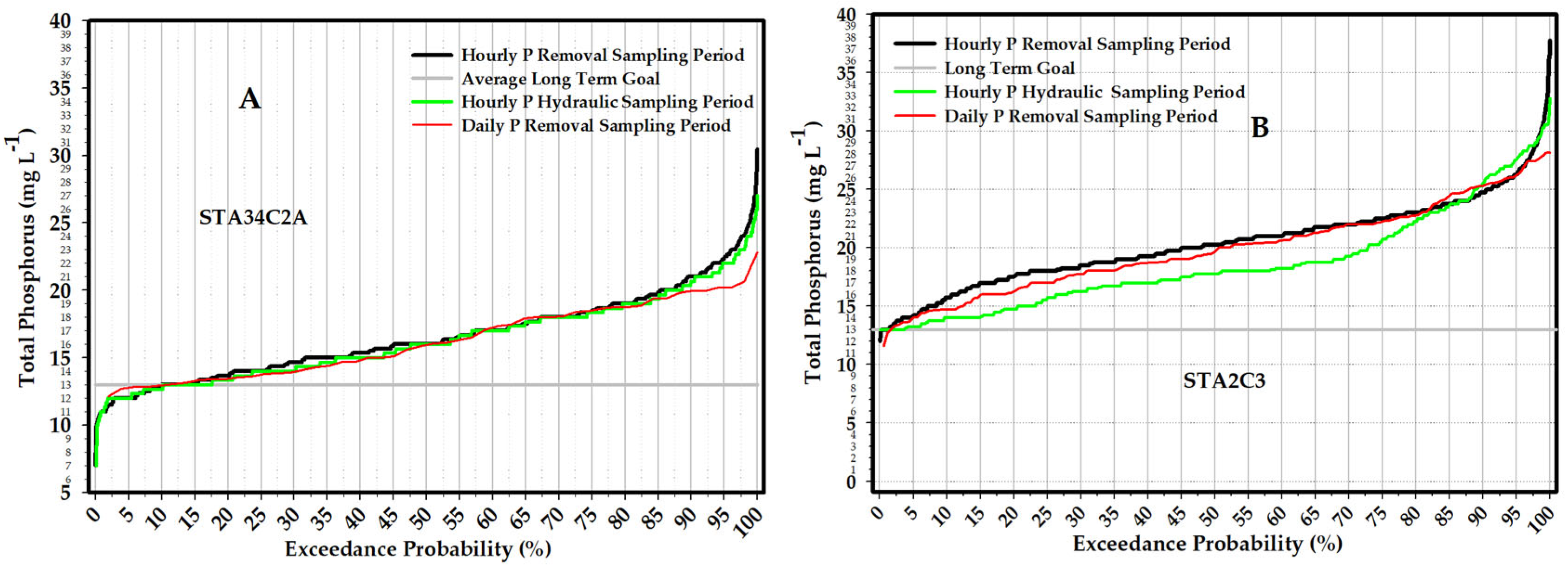
Exceedance probability plots are another tool to compare TP_out performance (Figure 10). STA34C2A clearly achieved TP_out values less than 13 µg L⁻¹ for almost 18% of the experiment time, regardless of the time period analyzed (hourly or daily) during both hydraulic P removal experiment periods (Figure 10A). In contrast, STA2C3 achieved TP_out values of 13 µg L⁻¹ for less than 3% of the experiment time (Figure 10B). A better performance in TP_out between 13 and 23 µg L⁻¹ for STA2C3 compared with STA34C2A was observed, which may be related to the wave frequency set during the experiment (Figure 10). A more recent study demonstrated higher dispersion (hydrodynamics and physical parameter) values with generated hydraulic waves [8] compared with steady state flow [35]. Dispersion is a key factor in spreading pollutants and nutrients in water bodies such as lakes, wetlands, and rivers/streams. We speculate that the observed high performance in STA2C3 (TP_out between 13 and 23 µg L⁻¹) during these experiments may have been caused by wave-generated high-dispersion values (Figure 10B).

The high phosphorus (P) removal performance observed in STA34C2A can primarily be attributed to the combination of its aspect ratio and vegetation density index (as detailed in Part 1), alongside its plug flow-type characteristics resulting from low hydraulic conductivity (K) values and high vegetation resistance (also discussed in Part 1). This is substantiated by the considerable number of observations indicating low P concentrations at the outflow (Figure 10A).

Despite STA2C3 having an aspect ratio twice as large as STA34C2A, the latter still achieved high P removal. This success is likely due to its aspect ratio in conjunction with the resident vegetation, specifically emergent aquatic vegetation (EAV) as opposed to submerged aquatic vegetation (SAV). The dense EAV type contributes to significant vegetation resistance, as evidenced by the low observed K values and vegetation index (Part 1), thereby fostering a plug flow regime.

Although median total phosphorus (TP) concentration values were comparable for the two time periods across both STAs (Table 1 and Table 2), observed TP concentrations were consistently lower in STA34C2A relative to STA2C3, suggesting superior P retention. In light of these variations in P retention, the aspect ratio (length/width) and vegetation type (EAV, SAV) warrant careful consideration in the design of future wetlands and the management of large, constructed wetlands.

Figure 8, Figure 9 and Figure 10 of Part 1 [12] show contour maps of arrival time at locations inside the cells. Porosity (i.e., plant density index) clearly demonstrates that vegetation resistance affects flow type and, consequently, TP removal performance. The observed change in TP concentrations in a treatment cell is likely to be lower at the outflow compared with the inflow and is determined, among other factors, by vegetation resistance or porosity (hydraulics). High and low porosity values [12] resulted in the observed high and low P retentions in STA34C2A and STA2C3, respectively.

4.1.3. Time of Sampling

RPA hourly sampling during the experiment revealed an interesting phenomenon, in which P concentration changed as a function of “hour of day” or sampling time (Figure 7 and Figure 8). This trend is clearly demonstrated at the outflow compared with the inflow sites and is also statistically significant among day and night hours. For example, for the t-test results at G377 (10:00 AM and midnight hour 23), the difference in the median values between the two groups is greater than would be expected by chance, i.e., there is a statistically significant difference (p = 0.002). The difference in the median values between the two groups (07:00 AM and midday/noon hour 12:00) at G377 is statistically significant (p = 0.002). However, the difference in the median values between the two groups at G377 (07:00 AM and midnight hour 23) is not statistically significant (p = 0.532). Meanwhile, the difference in the median values between the two groups (10:00 AM and midnight hour 23) at G378 is not statistically significant (p = 0.165). Also, the difference in the median values between the two groups (07:00 AM and midnight hour 23) at G378 is not statistically significant (p = 0.744). Yet, the difference in the median values between the two groups (07:00 AM and midday/noon hour 12:00) at G378 is greater than would be expected by chance, i.e., statistically significant (p = 0.019).

4.2. Hypothesis Testing and Interpretation of Results

This study was designed to evaluate the relative influence of physical and biogeochemical factors on P retention in large, constructed wetlands, testing the following hypotheses: the null hypothesis (H₀) postulates that there is no significant difference between the influence of physical parameters and biogeochemical factors on P retention, while the alternative hypothesis (H₁) proposed that physical parameters, specifically flow, transport, and water depth, exert a significantly greater influence on P retention than biogeochemical factors.

Our multi-regression model analyses, supported by high-frequency field data, strongly support the alternative hypothesis. The results indicate that physical parameters, particularly water depth, hydraulic residence time (HRT), and flow path characteristics, are the dominant drivers of P removal in this study. Among these, water depth and inflow TP concentration (TP_in) emerged as the most consistent and robust predictors of outflow TP concentration (TP_out) across both STA2C3 and STA34C2A. In contrast, simple linear regression revealed a weak or non-significant relationship between TPout and PLR, a key biogeochemical variable, suggesting that PLR alone has limited predictive power.

Additionally, lag time and HRT, both physical transport metrics, effectively accounted for phosphorus residence time, flow delays, and short circuiting within the systems, contributing to improved model performance. The type of vegetation and associated flow structures, such as EAV versus SAV, also played a significant role in shaping the hydrodynamics and, thus, phosphorus retention. Notably, STA34C2A exhibited superior TP removal performance despite its shorter flow path, likely due to the differences in vegetation and hydraulic structure. Furthermore, the field-based estimates of HRT closely matched modeled lag times, providing additional validation for the critical role of physical transport processes in phosphorus retention within constructed wetlands.

4.3. Hypothesis Evaluation

The collective findings of this study refute the null hypothesis (H₀) and provide strong support for the alternative hypothesis (H₁), demonstrating that physical parameters exert a greater influence than biogeochemical factors on P retention in large, constructed wetlands. This dominance of physical drivers was consistent across multiple sites, varying sampling frequencies, and diverse model configurations. Although biogeochemical factors such as the PLR contribute to the overall nutrient dynamics within the system, they were not the primary determinants of P removal efficiency. Instead, physical processes related to water movement, system geometry, and flow resistance, mediated by vegetation type and structural design, were found to be more critical in governing P retention.

These findings have important implications for the design, modeling, and management of large-scale treatment wetlands. First, hydraulic design and vegetation configuration should be prioritized to enhance plug-flow conditions and reduce short circuiting, which can compromise treatment performance. Second, monitoring strategies should incorporate high-resolution hydrologic data to effectively capture temporal variability in flow and transport processes. Finally, the use of lag-based metrics and hydraulic residence time (HRT) estimates derived from data association techniques offers a valuable approach for system assessment, performance optimization, and adaptive management.

5. Conclusions

Our study tested the following hypotheses:

• Null Hypothesis (H₀): There is no significant difference between the influence of physical parameters and biogeochemical factors on phosphorus retention in wetlands.
• Alternative Hypothesis (H₁): Physical parameters (flow, transport, and water depth) have a significantly greater influence on phosphorus retention in wetlands than biogeochemical factors.

Our results provide strong support for the alternative hypothesis (H₁). The analysis clearly demonstrated that physical parameters, particularly HLR, water depth, and HRT, exert a greater and more consistent influence on P removal performance in constructed wetlands than biogeochemical factors like PLR or internal biogeochemical cycling.

Constructed treatment wetlands, especially large STAs, are governed by a mix of controllable (e.g., HLR, water depth, and vegetation type) and uncontrollable (e.g., wildlife activity, storm events, and wind) factors. However, among these, physical and hydraulic controls consistently emerged as the most influential variables shaping TP outflow concentrations across diverse conditions and configurations.

Wetlands characterized by short travel distances and dominated by EAV provided optimum conditions that promote plug-flow hydraulics, and the optimization of HLR and HRT was found to be the most effective in achieving lower TP outflow concentrations. Conversely, in large, single-cell systems dominated by SAV, open water or sparse vegetation, water depth control, and reduction in short circuiting were the most critical physical variables. Despite similar HRT values between the two experiment sites, the wetlands with lower hydraulic conductivity (K) and dense EAV achieved superior P retention, highlighting the importance of hydraulic factors and flow path uniformity.

These findings refute the null hypothesis, as biogeochemical variables such as PLR did not significantly predict TP removal when evaluated alone, and their influence was secondary to hydraulic factors. Even when vegetation type indirectly influenced biogeochemistry, it did so through its primary effect on flow structure and retention time.

Moreover, our study introduced a novel application of data association techniques (cross-correlation analysis) to estimate effective HRT (HRT_P) in large wetland systems, demonstrating strong agreement with dye tracer experiments. This approach offers a practical, data-driven alternative for estimating residence time, which is a key variable in P removal modeling.

We also evaluated the impact of monitoring frequency. While hourly TP sampling revealed variability in outflow concentrations not captured by daily averages, this increased frequency did not improve overall P performance outcomes. However, it emphasized the importance of sample timing in system assessments, suggesting that synchronizing sampling with flow dynamics may be more cost effective than increasing frequency alone.

In summary, the evidence gathered supports the conclusion that physical drivers dominate P retention performance in constructed wetlands. Design and management strategies should prioritize hydraulic control (e.g., HLR, HRT, and water depth) and vegetation structure (EAV vs. SAV) to promote plug-flow conditions and reduce short circuiting. Managing controllable physical parameters offers the greatest potential for optimizing P removal in the face of variable biogeochemical processes and natural disturbances.