Article

Optimization of 3D Borehole Electrical Resistivity Tomography (ERT) Measurements for Real-Time Subsurface Imaging

Department of Geophysics, School of Geology, Aristotle University of Thessaloniki, 54124 Thessaloniki, Greece
Water 2025, 17(11), 1695; https://doi.org/10.3390/w17111695
Submission received: 30 April 2025 / Revised: 23 May 2025 / Accepted: 28 May 2025 / Published: 3 June 2025
(This article belongs to the Special Issue Application of Geophysical Methods for Hydrogeology—Second Edition)

Abstract

:
In this work, we explore the optimization of 3D Electrical Resistivity Tomography (ERT) measurement protocols for a 3D borehole grid configuration. Currently, there is no widely accepted standard measurement scheme for such setups. The use of numerous electrodes and the possibility of cross-borehole configurations lead to an extremely large number of potential electrode combinations. However, not all these combinations contribute significantly to the final resistivity model, and a complete measurement cycle requires substantial time to perform. This becomes particularly problematic in dynamic subsurface conditions, where changes may occur during data acquisition. In such cases, the measurements collected within a single cycle may reflect different subsurface states. Conversely, attempting to shorten acquisition time can result in too few measurements to resolve the subsurface structure at high resolution. Furthermore, most existing approaches assume a uniform half-space model and treat all measurements equally, failing to prioritize those that are most sensitive to actual subsurface changes. To address these challenges, we propose a 3D measurement optimization approach that yields an efficient acquisition scheme. This method produces inversion results comparable to those obtained from much larger datasets while reducing both measurement and processing requirements. Our optimization is based on a sensitivity-driven selection algorithm that accounts for the real subsurface structure rather than assuming a generic half-space. The proposed methodology is validated using synthetic data and tested with experimental data obtained from a laboratory tank setup. These experimental measurements were used to monitor permeation grouting; a technique applied to reduce permeability and/or increase the strength of granular soils through targeted injection.

1. Introduction

Permeation grouting has a long history, going back to the early 18th century, as hand pumps were used to inject a cement slurry into the gravel bases of dams to hinder water seepage [1,2]. Historically, grouting has been a ‘blind’ procedure: the grout cannot be tracked as it moves through the soil. While hand pumps have been replaced by electrical or diesel pumps and simple cement mixtures have been replaced by many chemical grouts or custom-made ultrafine cements, the injection procedure has seen little change over the centuries: an injection tool is inserted into ground, and either a sufficiently large volume of grout is injected or a pressure limit is reached, indicating clogging. Injection point density is designed based on an assumed shape around the injection point (generally spherical or column-shaped), from which a necessary density can be calculated to achieve sufficient coverage.
This is a costly procedure, as it requires a high density of injection points. There is no guarantee that the grout will be delivered in the designed shape. The success of the permeation grouting procedure can only be evaluated after finishing: the groundwater has ceased flowing, or it has not. If the created barrier is insufficiently impermeable, the procedure must be repeated. Since it is not clear where the leak is located, there is no guarantee that the second injection round will result in an impermeable barrier.
Traditional monitoring methods include borehole pressure measurements, core sampling, and visual inspection through test pits. While these methods provide direct information, they are often invasive, time-consuming, and spatially limited. Borehole pressure monitoring involves measuring the pressure within boreholes during and after grouting operations. This technique helps in understanding grout flow dynamics and ensuring the integrity of structures. Core sampling entails extracting cylindrical sections of soil or rock to analyze the subsurface conditions. This method provides direct evidence of grout penetration and the effectiveness of grouting in reinforcing geological formations. Visual inspection involves examining soil cuttings and core samples to classify soil types and detect changes in stratigraphy [3]. Geophysical methods, particularly Electrical Resistivity Tomography (ERT), have emerged as valuable non-invasive alternatives for real-time and volumetric monitoring. ERT is especially promising due to its sensitivity to changes in pore fluid conductivity and saturation, making it suitable for tracking grout spread and curing dynamics. Studies have shown its effectiveness in both laboratory [4,5] and field settings [6].
This research was performed specifically in the context of a novel iron-hydroxide-based chemical grout. The key chemical reaction is the oxidation of soluble Fe(II) into insoluble Fe(III). The iron in solution strongly increases electrical conductivity, making the grout traceable by Electrical Resistivity Tomography (ERT), especially in a real-time monitoring setup. The experiments were aimed at testing a new delivery principle as well, by making use of injections and extraction to force groundwater flow [7]. The techniques described in this paper are applicable to any grout provided it has a markedly higher electrical conductivity than the background groundwater.
The ERT real-time monitoring of grout flow opens many doors to improve the injection procedure:
  • The flow can be adjusted in real-time to force the delivery of the grout, when grout does not flow as designed.
  • Delivery can be evaluated in the short term. If necessary, a part of the target area can be treated immediately (rather than waiting for leaks to spring).
  • (Non-real-time): At a later point in time, the grout barrier can be located and evaluated and expanded or repaired if necessary.
Several papers demonstrate the usability of ERT monitoring in hydrogeophysics (i.e., [8]). Real-time monitoring is a hard task due to the time needed to collect and process measurements. Without real-time monitoring, injection proceeds “blind”, and optimization is impossible as the subsoil contains too much heterogeneity to produce regularly shaped grout curtains. This paper presents a scheme for optimizing the measuring arrays in 3D to allow the almost near-real-time monitoring of grouting.

2. Principles of Electrical Resistivity Tomography
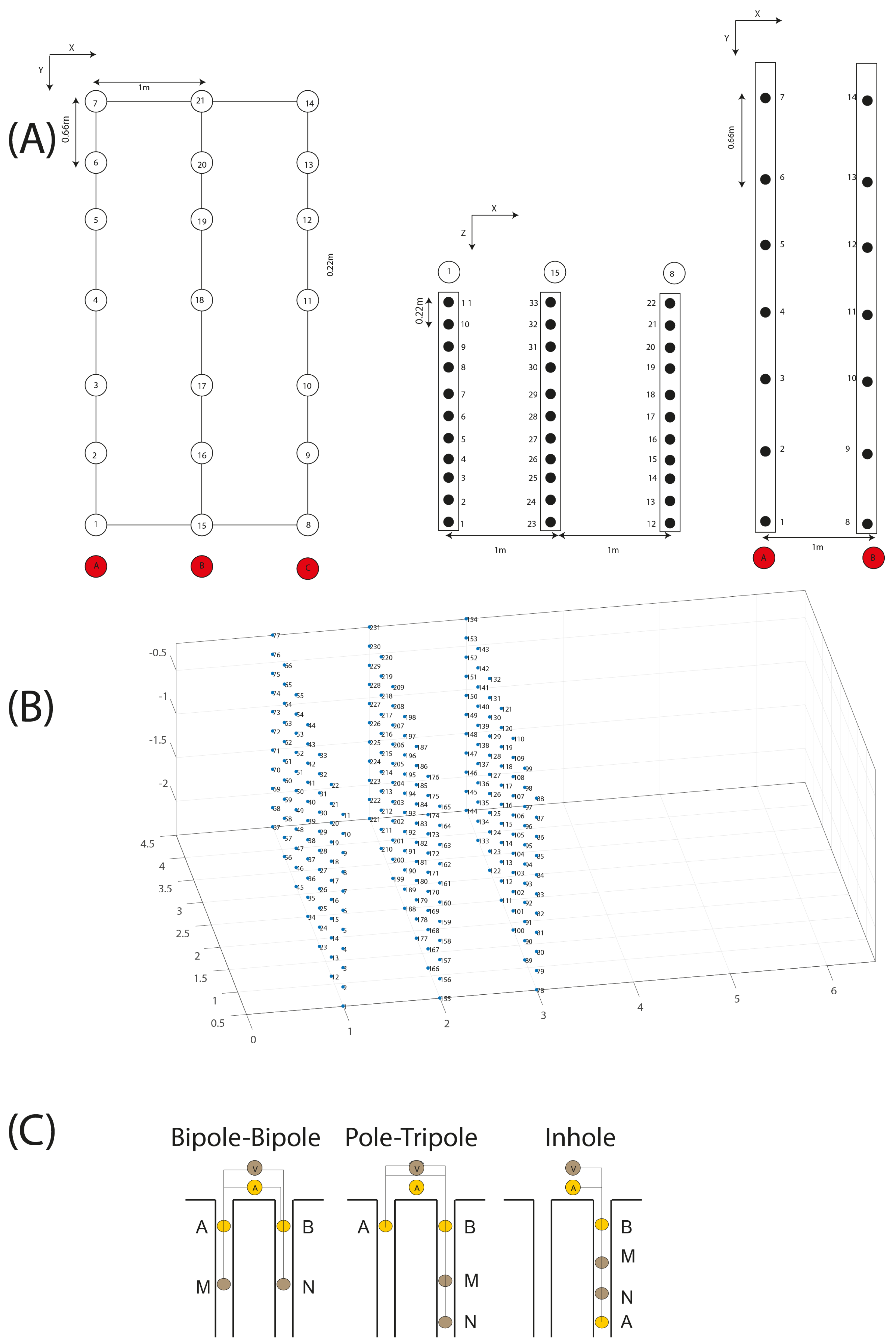
The ERT (Electrical Resistivity Tomography) method is a geophysical technique used to image the subsurface by measuring electrical resistivity. It involves deploying multiple electrodes on the ground surface to inject electrical current and measure the resulting voltage differences. The way in which the current and potential electrodes are arranged on the Earth’s surface is called an array. By changing the configurations of the array, the properties of the subsurface are mapped. An emerging field of application is he geoelectrical monitoring, which is increasingly used for assessing, among others, geotechnical, environmental, and hydrogeological processes [9]. Several geoelectrical instruments specially designed for monitoring are now in operation and allow the fast collection of large amounts of data which are then processed with special time-lapse inversion algorithms.
In this case, we consider 3D cross-hole ERT measurements. Although many cross-hole ERT array configurations have been proposed in the literature, there is not a standard measuring scheme that is considered optimum and thus there is no “standard practice” regarding array selection. Such methods have become common in geoelectrical prospecting and are used not only to replace any “standard” measuring configurations but, most importantly, to generate protocols in cases where no conventional ones exist, such as multiple boreholes installed in a 3D grid. An analogous situation exists for the 3D geoelectrical surveys, as a vast variety of electrode combinations is possible in 3D mode, and no standard practice exists for 3D ERT data collection. It follows that array optimization in the combined case of 3D and cross-borehole surveys can result in a vast number of possible measurements, so optimization is especially important as it can select a reasonable number of electrode combinations that can offer an improved resolution. Thus, optimizing arrays in 3D for monitoring experiments, with reducing acquisition time as a target, is not a well-studied case. This work contributes to optimizing 3D arrays and anticipates being used as a starting point.
The main advantage of using a measurement optimization approach is that it can produce protocols with a minimized amount of data without really sacrificing the overall geoelectrical imaging quality. This is a particularly important feature in many geoelectrical monitoring situations in which monitoring time and associated costs are important. Array optimization approaches follow an experimental approach, and they are either based on the model resolution matrix and a related goodness function [10,11,12,13] (3D and cross-hole arrays; 2015-long arrays) or they directly use the sensitivity matrix [14,15,16].
The idea of using optimized arrays in geoelectrical monitoring was recently extended to produce adaptive time-lapse optimized arrays, which change in every time-step to better map the geoelectrical changes. Such an approach has been proposed by [17,18]. Note that in our approach, we emphasize the reduction in acquisition time. We consider this experiment as a two-step measuring approach: a fast one that measures during the injection, where the acquisition time is reduced, and a second step after the injection, where we measure a more extensive dataset to image all features. In this work, we emphasize the first step.

3. Laboratory Test

In this section, we describe the actual grout injection principle and the steps we follow to monitor it in real-time. We used a three-step approach.
(1)
Numerical modeling to evaluate the optimum array (Section 4.1).
(2)
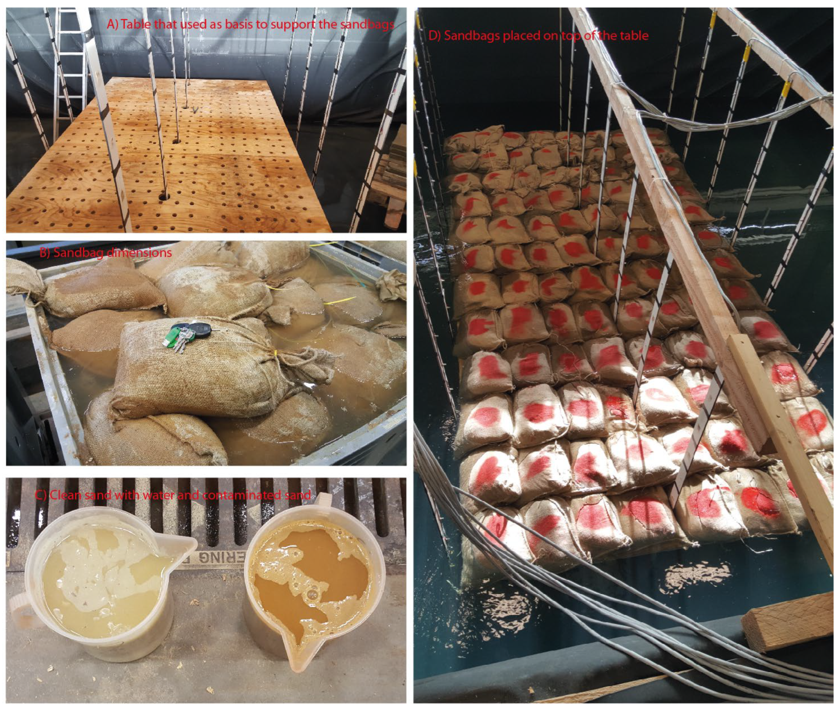
Evaluate the results with real data, collected from a tank filled with water. In the water-filled tank (Section 4.2), we placed a layer of sandbags (Section 4.4). We replaced a few of the sandbags with iron-grout sandbags and evaluated the performance of the reduced arrays.
(3)
We show the grout experiment data and results (Section 5).

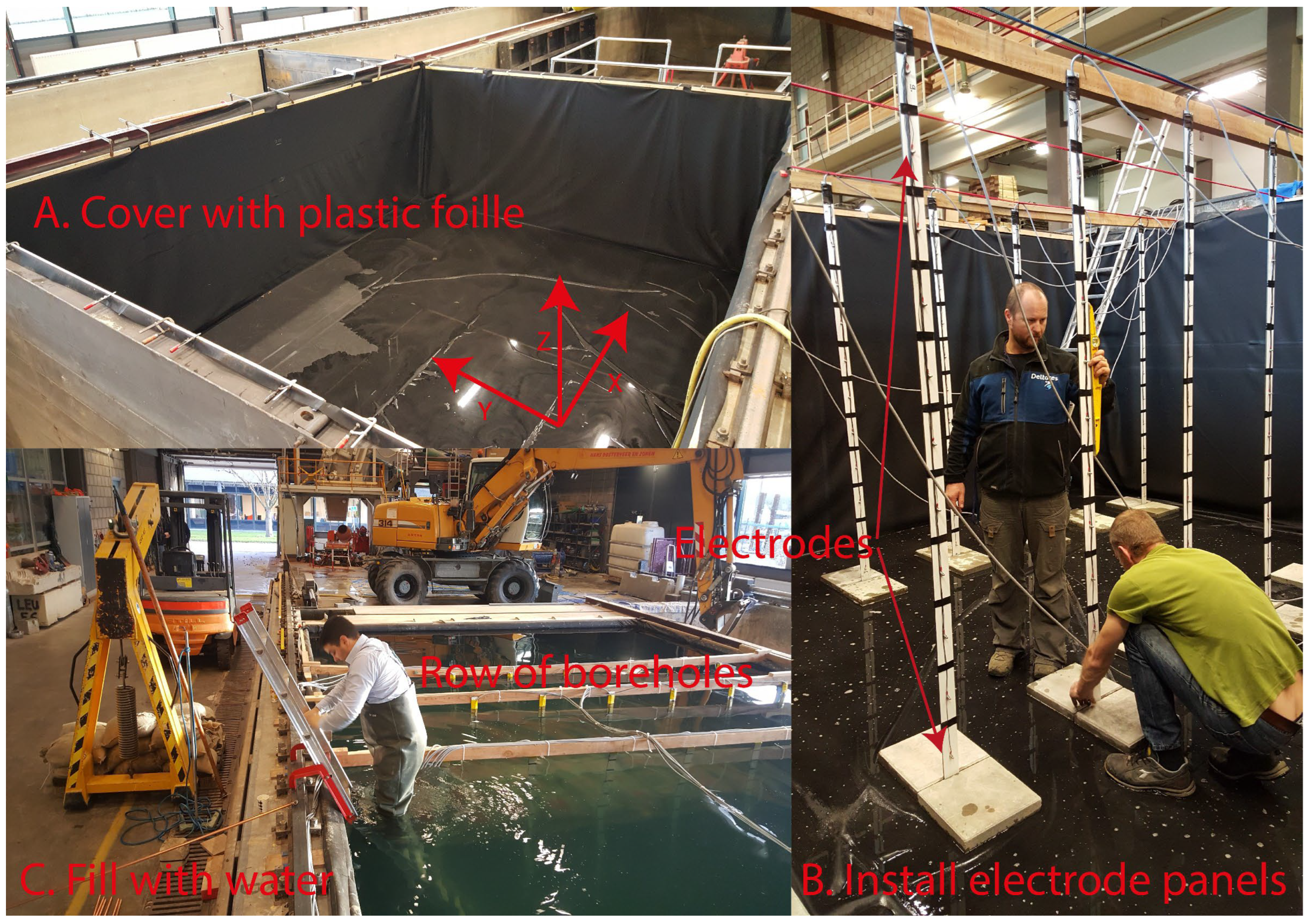
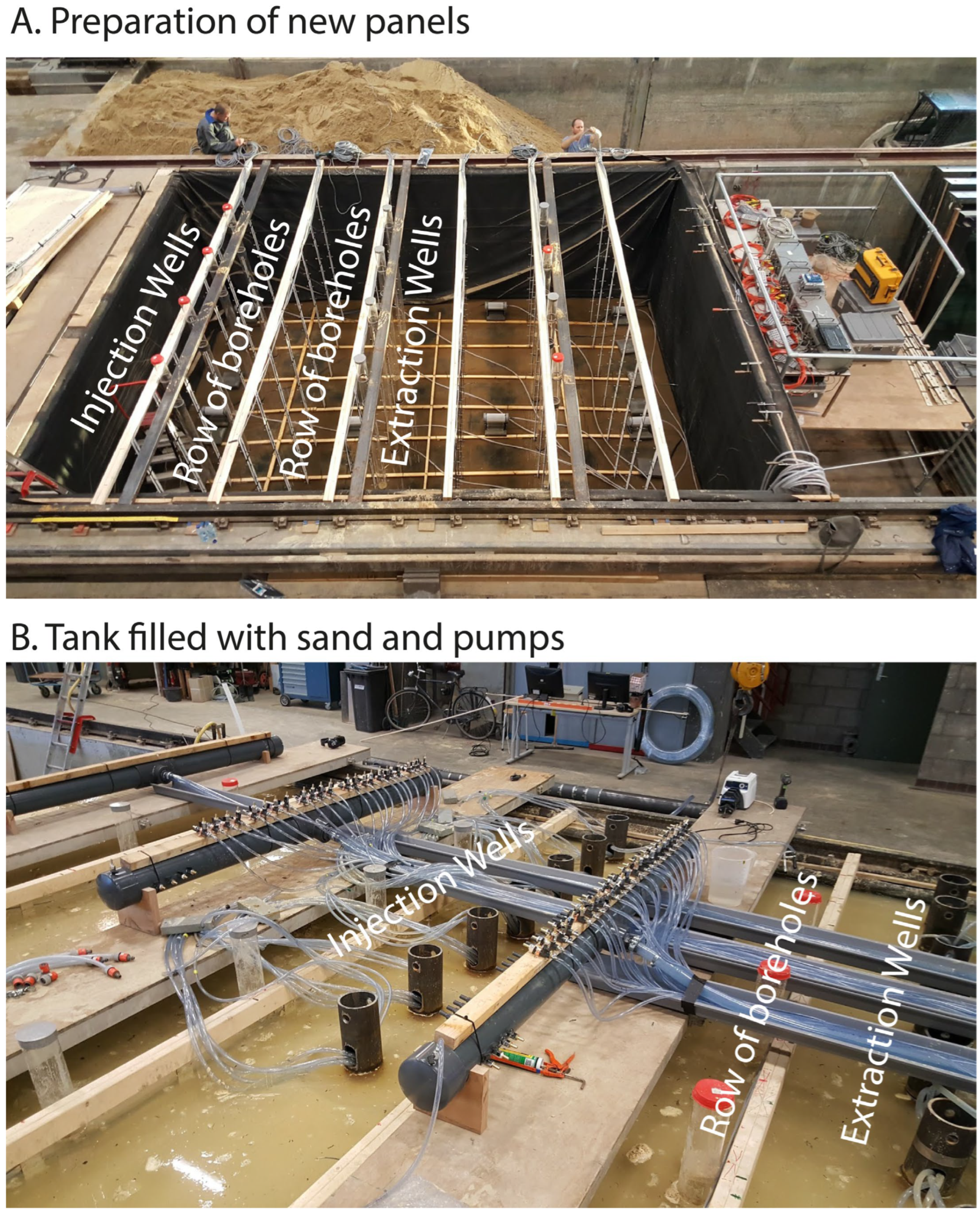
Details of the Lab Setup

The injection test took place in a 7 × 4.5 × 2.5 m tank. The sides of the tank were covered with a plastic foil (Figure 1A) before the installation of the test electrode panels (Figure 1B). Firstly, the tank was filled with water to ensure both waterproofing and electrical insulation from the surroundings (Figure 1C). The measured resistance between the tank interior and the external walls was of the order of 2 GOhm, suggesting full electrical insulation. During these initial trials, we installed only 3 rows of boreholes, with 7 boreholes per row, totaling 21 boreholes (Figure 2A). Each borehole has 11 electrodes with 22 cm of interspacing. Each electrode is an M8 stainless steel bolt, attached to the wooden frame. We ended up with 231 electrodes in total (Figure 2B). The array set used for measurement is a combination of bipole–bipole, pole–tripole, and inhole measures (Figure 2C).
The first step in the design of the acquisition setup is to detect the interspacing between the boreholes on the XZ plane. This step is the most crucial for the rest of the experiment, since it dictates the total number of borehole rows to be installed. The choice of the seven boreholes per row originates from the design of the actual injection system to be used in the field, where each borehole is also an injection needle. Thus, optimizing in the Y direction was not an option for this experiment. Note that we define two working planes, on the XZ plane and the XY plane (Figure 2A). This is because the length of each borehole on the XZ plane is 2.2 m, while if we consider the electrodes on the XY plane as electrodes belonging to a borehole, then the length is 4.5 m. This allows us to use that plane as a measuring plane and increase the resolution between the boreholes.
There are several authors describing the optimal distance between the boreholes with respect to the total length of the borehole and resolution (e.g., [11]), and we will not repeat it here. We note that high resolution in both the XY and XZ planes was required. Thus, we performed a numerical investigation of only the XZ plane to identify a thin target of 20 cm thickness and a width of 2 m (Figure 3). We simulate data for considering an optimal array of bipole–bipole, pole–tripole, and inhole measurements (Figure 1C), which totals 1150 measurements, in each plane (B1–B2, B2–B3, and B1–B3) (Figure 3). In the next section, we will discuss the optimization process per plane. Figure 3 shows the inversion results when we use data from both B1–B2 and B2–B3 against data from just B1–B3. It is obvious that the inversion image fails to correctly image the middle part accurately when only using data from the B1–B3 plane. The use of data from the XY plane might help increase the resolution on the center part, but it was decided to proceed with 1 m inter-borehole spacing due to the needs of this project.
Note that data are processed with three different types of software, [19,20,21], due to the different tasks of the project, 2D, 3D, or 4D inversion aspects, and access to the source code. For instance, we can easily extract the sensitivity matrix and statistics per measurement from IPI4DI, while in DCPRO, the 2D numerical modeling is more straightforward and robust, and RES3DINV is much faster than the other two to process the big 3D data, and it is the only code that can easily incorporate tank boundary conditions. Thus, the figures are not homogeneous between the different tasks. Yet, the inversion settings remained similar among all types of software, and they are based on an iterative gradient-based algorithm using a 4D inversion scheme, with the same level of fitting and stopping criteria (a less than 2% improvement between two subsequent iterations) and an automated damping value based on the l-curve. Mesh is based on orthogonal (in 2D) or hexagonal (in 3D) structures with the same area or volume across the inversion domain. More information about the inversion settings can be found in [21]. We mention here that the inversion RMS was around 3%, which is a rather low value given the level of complexity.

4. Optimization in Water Tank

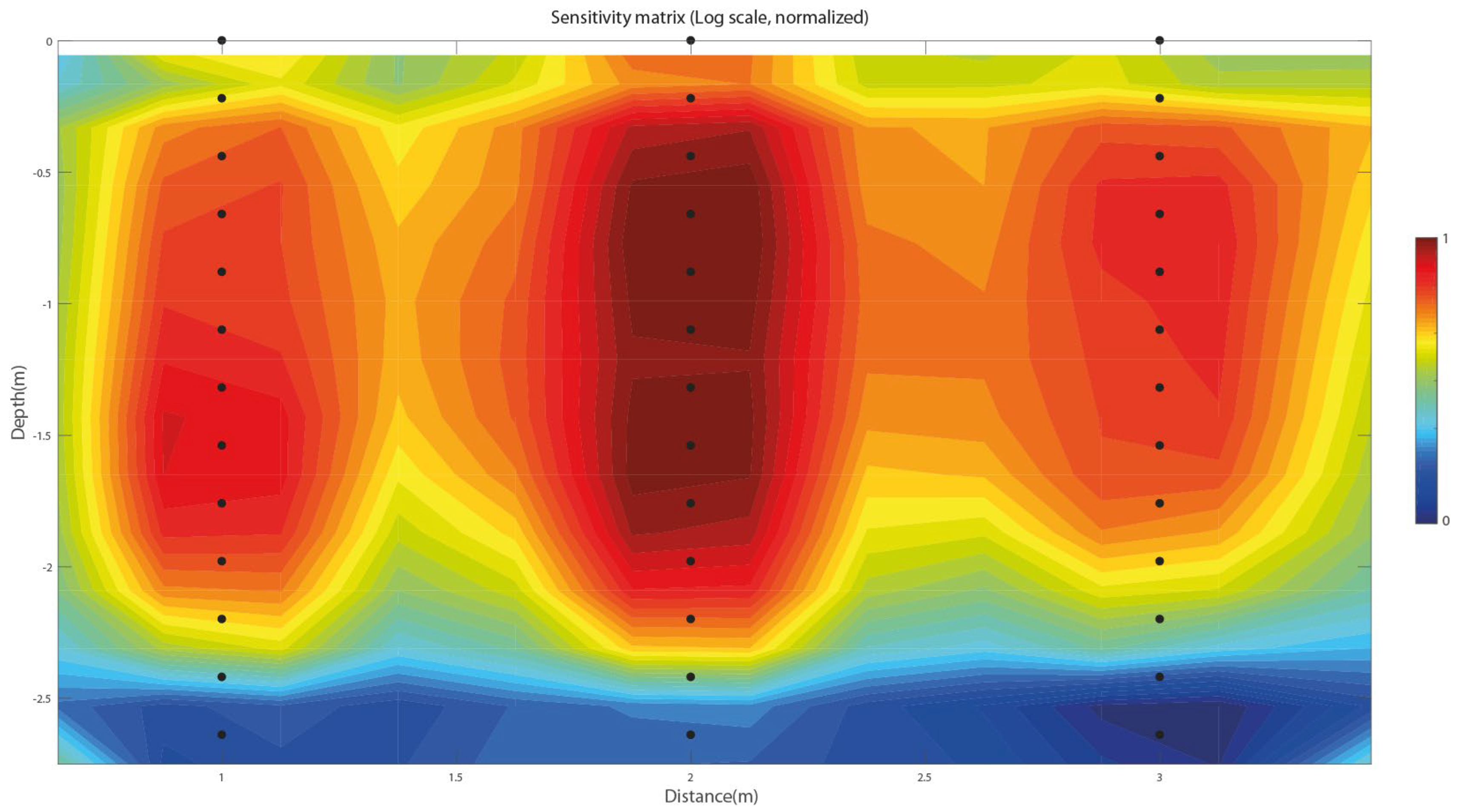
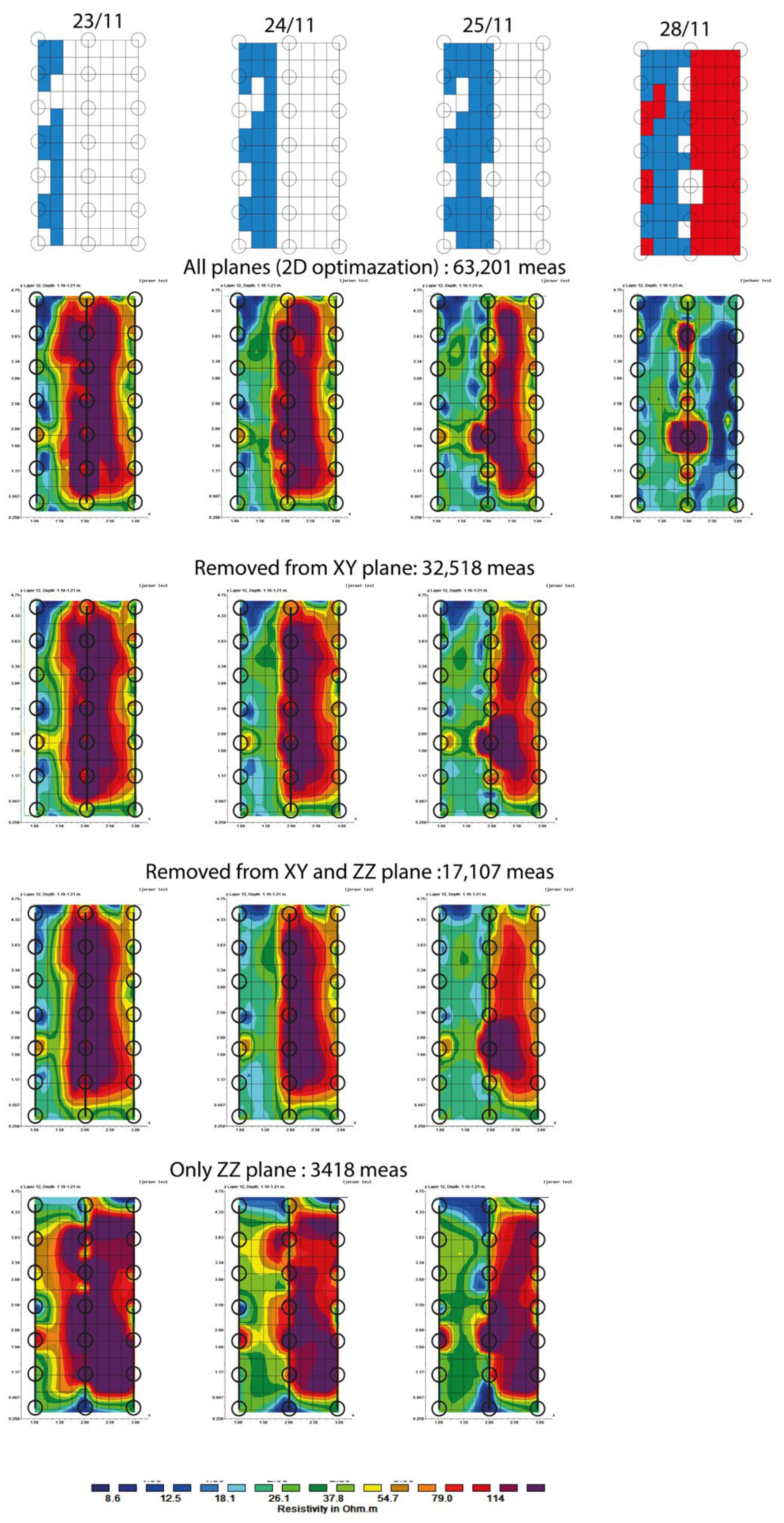
4.1. Optimization in 2D Planes (Numerical Modeling)

In the proposed work, the array optimization technique is based on the Jacobian matrix method [22,23], and it is the standard approach used in the optimization process. The approach requires that optimization is carried out by selecting measurements based on their resolution matrix value in relation to the subsurface parameters. The resolution matrix provides a measure of how well the inversion process can recover the true model parameters from the observed data. Ideally, the resolution matrix would be the identity matrix, indicating perfect resolution where each model parameter is recovered independently and without influence from others. However, in practical scenarios, the resolution matrix typically deviates from the identity, reflecting limitations in the data and the inversion setup. The diagonal elements of the matrix indicate how well individual parameters are resolved—values close to one signify high resolution, while values much less than one suggest poor resolution. Off-diagonal elements show the degree of parameter mixing, where the estimate of one parameter is influenced by others, leading to smearing or artifacts in the final model.
Firstly, a dataset involving a large number of possible electrode combinations is formed, and then, only the measurements that have a geometrical factor lower than the selected threshold are kept, forming the comprehensive dataset. The geometrical factor is a number that compensates for the different array distances between the electrodes.
G = ( 1 A M 1 B M 1 A N + 1 B N )
Subsequently, the subsurface corresponding to the particular electrode arrangement is parametrized, and the Jacobian matrix is calculated for every measurement and parameter. For every parameter, we select, uniquely, the measurements which exhibit the largest absolute value of sensitivity, and we include them in the optimized dataset. This procedure will result in at least as many measurements as the model parameters and can be repeated iteratively.
To obtain more information about the areas with lower resolution, the parameters are ranked based on their Jacobian norm, and then more configurations are chosen from the parameters, which have smaller norms (viz., they are less resolved). This procedure makes the algorithm less time-consuming since there is no need for calculating the resolution matrix, and moreover, tests have shown that it produces results equivalent to the resolution matrix-based optimization schemes [24]. This approach has been extensively tested with synthetic models and in the field. In this work, we expanded this approach in 3D to see the effects on measuring in different planes, such as (XY, XZ, XX, YY, ZZ, and XZ). A cumulative sensitivity matrix (2D plane) for the optimized arrays is shown in Figure 3. Note that due to the optimization procedure, the cumulative sensitivity matrix is not fully symmetrical. Note that the aim of this work is to be able to image the area where we expect changes (in our setup, around −1.5 m), and thus the areas with lower resolution values are of no importance. This is a crucial step to decrease the acquisition time.

4.2. Lab Test (Evaluation with Real Data)

Prior to the injection, we evaluated the performance of the borehole location uncertainties, electrode condition, and sensitivity test by performing a static study. That is in the tank, we installed a wooden table with holes every 10 cm in both X and Y directions so that the table is a porous medium (Figure 4A). As a first try, we performed a 2D acquisition of boreholes 4-18-11 to see the effect of the table (Figure 4A) using the conventional pole–tripole skip 1,2,3 [24], bipole–bipole, and the combination of them. Note that we left the table for 48 h in the tank filled with water before the start of the tests. All arrays worked reasonably well (with RMS in the order of 5%), whereas bipole–bipole seemed to produce more artifacts. Inversion results showed that the resistivity of the table is ~75 Ohm·m (Figure 5). Since the optimization in 2D is trivial, we will not repeat the steps we followed here (you can read more in the cited papers). We ended up with an array of 1150 measures per place (i.e., measure between the three boreholes, as shown in Figure 3), which is the basis of the 3D optimization further down.
Then, on top of the table, we placed sandbags initially filled with clear sand (Figure 4D), and later we replaced a few of them with iron-filled sandbags that were used in previous tests and had iron material. Note that the iron–sand-filled sandbags came from many different experiments, and it was not possible to confirm that the iron content was consistent in each bag. We first measured the bulk resistivity of the sand sample saturated with tap water (Figure 4C, left), and we found that it was ~80 Ohm·m. The water conductivity was 22 Ohm·m at 21 °C. The bulk resistivity of the sand saturated with iron was about ~3 Ohm·m (Figure 4C, right). This step gave us an indication of the contrast of resistivity that we can expect.

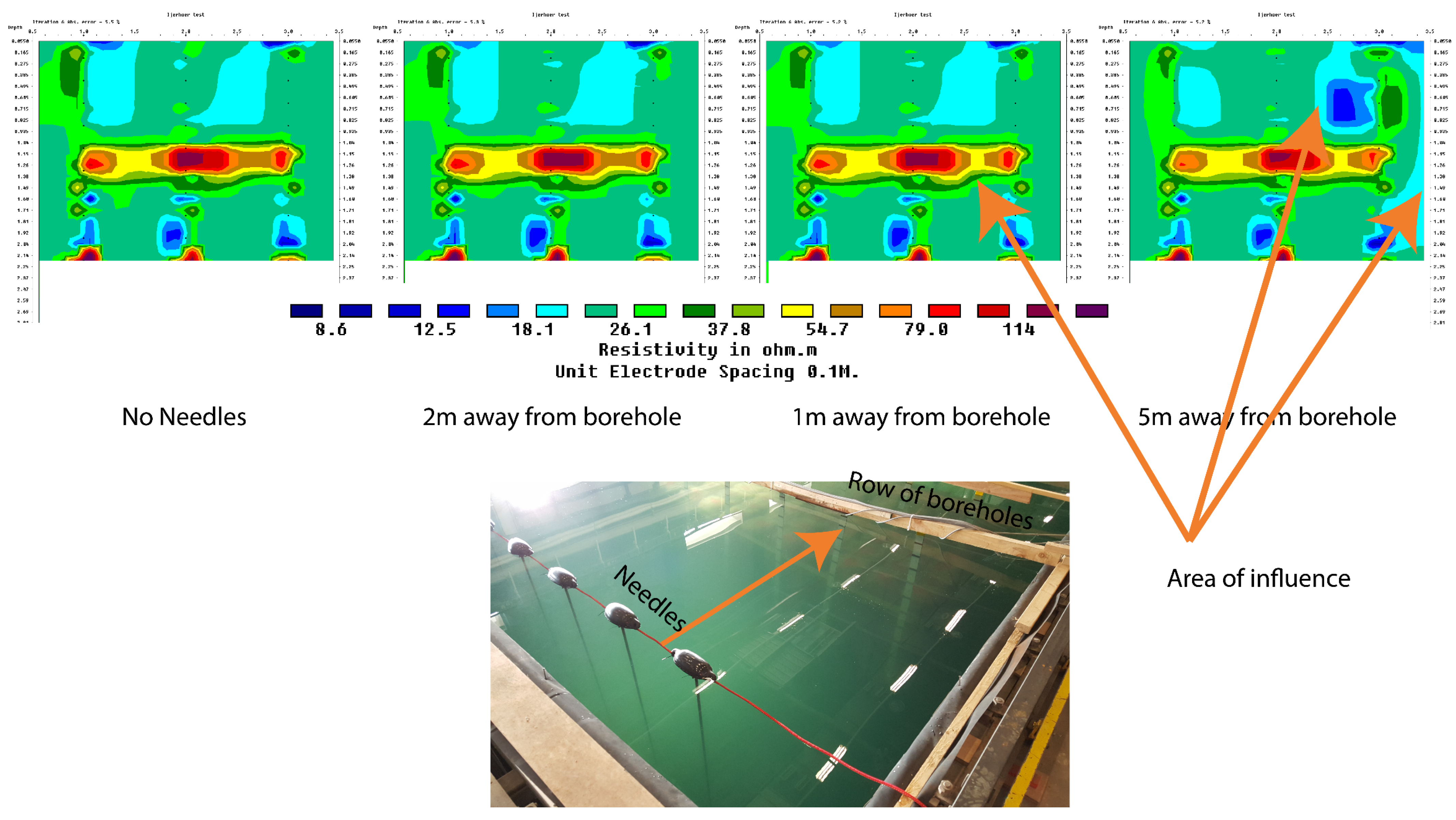
4.3. Effects of Additional Equipment

Additional tests were performed to investigate the effects of the injection needles and metal structures in the vicinity of the boreholes. We installed seven metal spikes, representing the needles, and measured the tank filled with water and the presence of the table (Figure 6). The spikes were not connected to each other (closing a circuit), which is representative of an actual setup. The table was used as a base to support the sandbags (see next section). First, we measured without the needles, and then with the needles, at 2 m, 1 mm, and 0.5 m distances from the measuring boreholes, respectively. We did not observe any influence when the needles were 2 m, minor influence at 1 m, and significant influence at 0.5 m. This is shown with a low resistivity body on the upper right corner (Figure 6). The RMS error varied from 5.2 to 5.5% for all four tests. We concluded that a safe distance of 1 m between the measurement boreholes and needles should be maintained for the rest of the experiment. Note that the choice of 1 m is also based on the limited dimensions of the tank: We need a safe distance from the tank walls to avoid boundary effects that do not reflect in field tests and enough distance to install three rows of measures. In field setups, the choice of a safe distance can be greater. Also, note that from this point on, we switched the processing software to RES3DINV v3.18. This is due to the fine mesh we used for the processing of the full-time-lapse algorithm. RES3DINV was at that time the only software that could process the data fast enough.

4.4. Sandbag Tests—Results

The pseudo-time-lapse study was performed as follows. Bags were marked based on whether they contained clean sand or ironsand (Figure 4D). Based on the sketch (Figure 7, top row), we replaced the sandbags with iron bags and performed a full round of measurements on four different days (23, 24, 25, and 28 of November). We had at least 24 h between each experiment to ensure that the newly placed bags were fully saturated. The array used per plane had 1150 measurements, as discussed in Section 3. We measured the following planes (see Figure 2A).
(a)
On the XZ plane, for instance, between 1 and 15 boreholes (i.e., row A and B) and also between 15 and 8 (i.e., row B and C).
(b)
On the XY plane, in two directions, for instance, 1 and 16 and 2 and 15.
(c)
On the ZZ plane, for instance, between A and B and also between B and C.
Note that a full array with all combinations has 200,895 measurements if no optimization is considered. The acquisition time for this array was more than 18 h, and thus, we do not have a complete set of all the data. Rather, as a basis, we used the optimized dataset per plane (as discussed), which has 63,201 measurements, and the acquisition time is about 6 h. We did not include measurements on the ZX and YY planes, as this would add to the acquisition time, with the gain in information expected to be small. Since this is a 3D optimization, we present the results in two steps, first by removing planes with measurements (reducing the 3D coverage but maintaining the 2D array) and then by removing the measurements from all planes (reducing measurements per 2D plane while maintaining the 3D coverage). Note that the goal for this project is the reduction in acquisition time and not only finding the optimal array. That is, if an array can resolve the features in the shortest acquisition time reasonably well, it is prioritized in our work. This is due to the need to map in as real-time as possible during the injection so that the operator of the injection knows where the iron wall is located. Once the injection process is finished, the measuring sequence can use one of the more extensive datasets to better image the subsurface. Note that each measurement was repeated two times, so we can have a standard error deviation in measurement.
The semi-time-lapse model is shown in Figure 7. The whiteboards indicate the sandbags with clean sand (high resistivity) while the blue boards show iron bags. We measured at four different time-steps, 23, 24, 25, and 28 November. After each placement of the bags, we waited for 24 h before starting the measurement sequence to allow the sandbags some time to be fully saturated. At the end of each measurement, the water level was dropped below the sandbag level until the beginning of the next round of measurements. This way, we minimized dissolving the iron in the water. At the end of the 25 of November, we left the iron bags in the tank filled with water. Thus, on the 28th, we observed that part of the iron from the sand was dissolved in the water, and the right part of the sandbags had significantly lower resistivity. We also observed a change in the resistivity values from the bags on the left side due to the iron dissolved in the water. Even though the array can still capture the features, we decided to exclude it from further processing. Including quantitative metrics would greatly enhance the interpretation of the results. In fact, identifying appropriate metrics proved to be a challenge for us. In the case of lab experiments, the main difficulty lies in evaluating the model’s performance meaningfully. The commonly used model RMS error is insufficient, as it also captures differences in resistivity values, which span a wide range—even on a logarithmic scale. For instance, calculating the RMS difference for each pixel between a sandbag (80 Ohm·m) and an iron bag (2 Ohm·m) inherently gives unequal weight to each material, and we also lack precise information about the iron concentration within each bag. A potentially more suitable approach might involve assessing the similarity between the reconstructed and reference images—a direction we consider promising for future work. In this work, the evaluation is based on visual inspection, as this is what would happen in traditional inspection work. We chose not to include ratio images in our analysis because the background in our experiments was homogeneous—composed either of water or sand—and we felt that such images would not contribute additional insights. However, in field scenarios where subsurface heterogeneity plays a significant role, ratio images could offer a more effective means of visualizing the results.
Removing the measuring planes in the XY direction did not end up changing the spatial resolution significantly (i.e., the level of detail at which we can image the target), and while reducing measurements from the planes XY and ZZ simultaneously, we observed a significant decrease in spatial resolution. Using measurements only from the ZZ plane, we observed that the actual distribution of sand/iron bags cannot be accurately imaged (Figure 7). We conclude from this step that the XX and ZZ planes are sufficient to measure.
Figure 8 shows a further reduction in measurements per plane, as discussed in Section 3. The criteria are based on the number of measurements to be maintained per cell per 2D plane. It shows that by reducing the measures by 40% (see Figure 8, results with 39,774 measurements), we end up with similar results. The 3D coverage of the boreholes partially compensates for the reduced measurements. Further reducing the measurements by 85%, we observe that the inversion results fail to properly image the subsurface.
With further testing, we concluded that a reduction of 40% per plane, while removing the XY plane measurements (Figure 9), results in a reasonably well-reconstructed image of the subsurface. The main features, as indicated by the red ellipse, are present, just less pronounced. Particularly, the sandbags on 25 November on the upper left side are imaged with a satisfactory contrast (more than 10 Ohm·m), making them easy to distinguish, considering that it is a time-lapse study. Plotting the ratio changes rather than the actual values helps identify the changes more easily. Ratio plots are used in the next section.

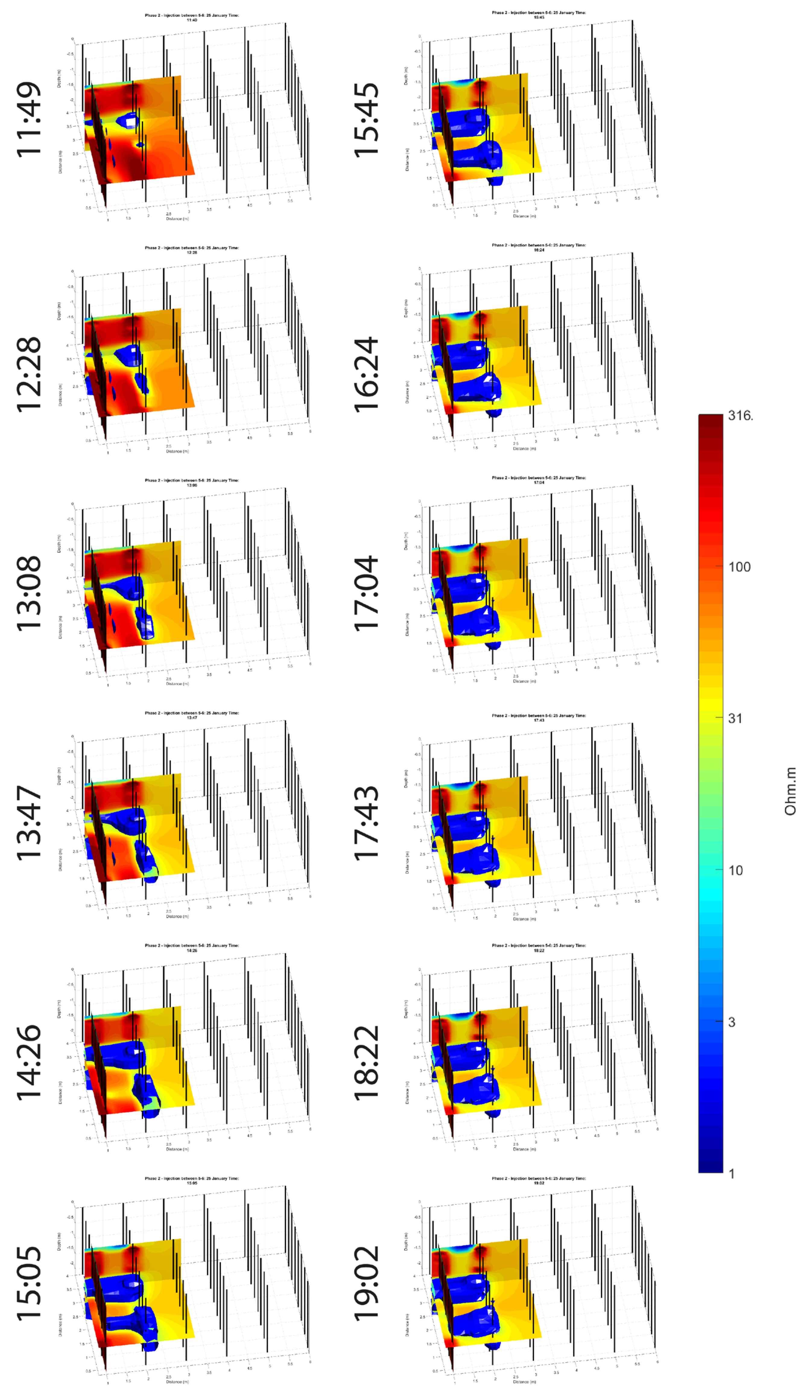
5. Injection Test—Results

During the next step of the experiment, we installed six planes of boreholes (inter-borehole spacing of 1 m), with eight boreholes per lane (Figure 10). The choice of the extra borehole was decided due to a change in the schedule of the injection tests. Two rounds of tests took place, once in the upper part of the tank and once in the lower part of the tank. Thus, we used boreholes 1 to 5 in the first round and boreholes 4 to 8 in the next round (Figure 10A). The upper part of the tank was used for a different chemical injection, and we will not show the results here. The injection took place in pairs A-B, B-C, and C-D of planes (Figure 10A). This means that the injection and measurement planes are
  • A-1-2-B;
  • B-3-4-C;
  • C-5-6-D.
In other words, when injection was between A and B, we utilized boreholes 1–2, and when injection was between B-C, we utilized boreholes 3–4, etc. Thus, we measured only between two borehole planes at a time, rather than three planes like the numerical data shown above.
Figure 11 shows the complete tank when empty and when filled with sand and all the equipment needed for the experiment. We ran the optimization algorithm, and we ended up with 3479 measurements with 21 min of acquisition. Due to hardware limitations, it was not possible to remove repetition of each measurement (i.e., stacking). Thus, each array was measured twice (to obtain the std error of each measure), and consequently, the acquisition time could be reduced to ~11 min. Then, the tank was filled with sand, and injection needles and pumps were installed (Figure 11B). Note that we optimized the array to complete a full round of measurements with electrodes that belonged to one borehole, before it proceeded to the next pair. In other words, all measurements that used borehole 1 were measured sequentially; then, the array moved to measurements with all electrodes belonging to borehole 15, etc. It was an extra effort to reduce the changes in the subsurface, which might happen within a plane that uses this same borehole during the measurements.
Figure 12 shows snapshots of the time-lapse images, when injection takes place between panels A and B, every 21 min. In this injection scenario, we observed that the ironwater flow did not spread in a layered sense but rather it flowed along the path from pump to pump, leaving “blanks”. Different compositions of the iron wall took place between 2 and 3 injections and also between 3 and 4 injections, but we will not show the results in this work. After all, the experiments were measured with all planes (one plane at a time, then switching to the next and merging the measurements) using the same array protocol as the monitoring one (Figure 13). After using an excavator, we removed sand by making a trench in the tank, and we observed a good match between the inversion results and the actual location of the iron material, where gaps and the preferential flow paths were aligned with the inversion results.

6. Conclusions

In this work, we presented a workflow for monitoring lab tests using an ERT system. We tested both the simulation results and tank results to further understand the effects of the noise and geometry errors of the boreholes. Much of the effort for this test was spent on the electrical insulation of the tank, a time-consuming part. In our work, we present a good agreement between the simulated protocols and the actual measurements, indicating that the simulation step is still a good approach for the beginning of the design. During our efforts, we managed to reduce the acquisition time to 21 min (or 10.5 if we remove the repeated measurements), indicating that almost real-time monitoring is possible. Note that the final acquisition time needed is heavily dependent on the field’s needs. Following this workflow, it is possible to further reduce the acquisition time, with some sacrifice on the spatial resolution. Yet, this workflow ensures that the best possible dataset will be collected. Notice that in this workflow, we emphasize minimizing the acquisition time and maintaining a similar spatial resolution. A 3D time-lapse optimization of the ERT array is a far more complex procedure, but at the same time, it has more degrees of freedom to optimize. There are several planes to be considered, and not all measuring planes contribute positively. This helps with the reduction in measurements, especially if time is crucial. Note that the actual field setup (i.e., number of electrodes needed, distance between boreholes, installation depth, etc.) is heavily dependent on the needs of the monitoring target. We propose this flowchart as a workflow to optimize the monitoring procedure.
Yet, the reduction in time could also be improved at a hardware level using machine learning techniques during the acquisition. In such a scenario, the system would be learning automatically based on the relative changes per measurement, allowing us to only measure where changes occur and fill the gaps of the missing measurements from the simulation [25]. This is work in progress.

Funding

This research received no external funding.

Data Availability Statement

The original contributions presented in this study are included in the article. Further inquiries can be directed to the corresponding author.

Acknowledgments

We thank Wim de Lange for the idea of using geophysical methods to monitor the grouting process and various colleagues in Deltares for the help and advice on how to make the lab test.

Conflicts of Interest

The authors declare no conflict of interest.

References

  1. Li, Q.; Li, Q.; Wu, J.; Li, X.; Li, H.; Cheng, Y. Wellhead Stability During Development Process of Hydrate Reservoir in the Northern South China Sea: Evolution and Mechanism. Processes 2025, 13, 1630. [Google Scholar] [CrossRef]
  2. Li, Q.; Li, Q.; Cao, H.; Wu, J.; Wang, F.; Wang, Y. The Crack Propagation Behaviour of CO2 Fracturing Fluid in Unconventional Low Permeability Reservoirs: Factor Analysis and Mechanism Revelation. Processes 2025, 13, 159. [Google Scholar] [CrossRef]
  3. U.S. Army Corps of Engineers (USACE). Grouting Technology Manual; EM 1110-2-3506; USACE: Washington, DC, USA, 1995.
  4. Chambers, J.E.; Gunn, D.A.; Wilkinson, P.B.; Meldrum, P.I.; Haslam, E.; Holyoake, S.; Kirkham, M.; Kuras, O.; Merritt, A.; Wragg, J. 4D electrical resistivity tomography monitoring of soil moisture dynamics in an operational railway embankment. Near Surf. Geophys. 2014, 12, 61–72. [Google Scholar] [CrossRef]
  5. Uhlemann, S.; Chambers, J.; Falck, W.E.; Tirado Alonso, A.; Fernández González, J.L.; Espín de Gea, A. Applying Electrical Resistivity Tomography in Ornamental Stone Mining: Challenges and Solutions. Minerals 2018, 8, 491. [Google Scholar] [CrossRef]
  6. Uhlemann, S.S.; Chambers, J.E.; Meldrum, P.I.; Wilkinson, P.B.; Gunn, D.A.; Hutchinson, D.; Swift, R.; Dijkstra, T.A.; Kuras, O. Imaging of Moisture Dynamics within an Operational Railway Cutting—The Effects of Vegetation. 2016. Available online: https://www.earthdoc.org/content/papers/10.3997/2214-4609.201602050 (accessed on 27 May 2025).
  7. De Lange, W.; Vink, J.P. A Method to Create a Horizontal Resistance Layer by Injection of a Viscous Fluid: PLAID. Ground Water 2018, 56, 541–546. [Google Scholar] [CrossRef] [PubMed]
  8. Revil, A.; Karaoulis, M.; Johnson, T.; Kemna, A. Review: Some low-frequency electrical methods for subsurface characterization and monitoring in hydrogeology. Hydrogeol. J. 2012, 20, 617–658. [Google Scholar] [CrossRef]
  9. Loke, M.H.; Chambers, J.E.; Rucker, D.F.; Kuras, O.; Wilkinson, P.B. Recent developments in the direct-current geoelectrical imaging method. J. Appl. Geophys. 2013, 95, 135–156. [Google Scholar] [CrossRef]
  10. Stummer, P.; Maurer, H.; Green, A. Experimental design: Electrical resistivity data sets that provide optimum subsurface information. Geophysics 2004, 69, 120–129. [Google Scholar] [CrossRef]
  11. Wilkinson, P.B.; Meldrum, P.I.; Chambers, J.E.; Kuras, O.; Ogilvy, R.D. Improved strategies for the automatic selection of optimized sets of Electrical Resistivity Tomography measurement configurations. Geophys. J. Int. 2006, 167, 1119–1126. [Google Scholar] [CrossRef]
  12. Wilkinson, P.B.; Chambers, J.E.; Lelliott, M.; Wealthall, G.P.; Ogilvy, R.D. Extreme sensitivity of crosshole electrical resistivity tomography measurements to geometric errors. Geophys. J. Int. 2008, 173, 49–62. [Google Scholar] [CrossRef]
  13. Wilkinson, P.B.; Loke, M.H.; Meldrum, P.I.; Chambers, J.E.; Kuras, O.; Gunn, D.A.; Ogilvy, R.D. Practical aspects of applied optimized survey design for electrical resistivity tomography. Geophys. J. Int. 2012, 189, 428–440. [Google Scholar] [CrossRef]
  14. Furman, A.; Ferré, T.P.A.; Warrick, A.W. Optimization of ERT surveys for monitoring transient hydrological events using perturbation sensitivity and genetic algorithms. Vadose Zone J. 2004, 3, 1230–1239. [Google Scholar] [CrossRef]
  15. Hennig, T.; Weller, A. Two-dimensional object-oriented focusing of geoelectrical multi-electrode measurements. In Proceedings of the 11th Meeting of the EAGE Near Surface Geophysics Conference, Palermo, Italy, 4–7 September 2005. [Google Scholar]
  16. Athanasiou, E.N.; Tsourlos, P.I.; Vargemezis, G.N. Optimizing electrical resistivity array configurations for hydrogeological studies. In Proceedings of the TIAC’07 International Conference on Technology of Seawater Intrusion in Coastal Aquifers, Almeria, Spain, 16–19 October 2007. [Google Scholar]
  17. Wilkinson, P.B.; Uhlemann, S.; Meldrum, P.I.; Chambers, J.E.; Carrière, S.; Oxby, L.S.; Loke, M.H. Adaptive time-lapse optimized survey design for electrical resistivity tomography monitoring. Geophys. J. Int. 2015, 203, 755–766. [Google Scholar] [CrossRef]
  18. Tsakiribaloglou, K.; Tsourlos, P.; Vargemezis, G.; Tsokas, G. An Algorithm for the Adaptive Optimization of ERT Measurements. In Proceedings of the Near Surface Geoscience 2016-22nd European Meeting of Environmental and Engineering Geophysics, Barcelona, Spain, 4–8 September 2016. [Google Scholar]
  19. Loke, M.H. Res2Dinv ver. 3.59 for Windows XP/Vista/7: Rapid 2-D Resistivity & IP Inversion Using the Least-Squares Method; Geoelectrical Imaging 2D & 3D; Geotomo Software: Gelugor, Malaysia, 2010. [Google Scholar]
  20. Kim, J.-H.; Yi, M.J.; Park, S.G.; Kim, J.G. 4-D inversion of DC resistivity monitoring data acquired over a dynamically changing earth model. J. Appl. Geophys. 2009, 68, 522–532. [Google Scholar] [CrossRef]
  21. Karaoulis, M.; Revil, A.; Tsourlos, P.; Werkema, D.D.; Minsley, B.J. IP4DI: A software for time-lapse 2D/3D DC-resistivity and induced polarization tomography. Comput. Geosci. 2013, 54, 164–170. [Google Scholar] [CrossRef]
  22. Tsourlos, P.; Jochum, B.; Supper, R.; Ottowitz, D.; Kim, J.H. Optimizing Geoelectrical Arrays for Special Geoelectrical Monitoring Instruments. In Proceedings of the Near Surface Geoscience 2016-22nd European Meeting of Environmental and Engineering Geophysics, Barcelona, Spain, 4–8 September 2016. [Google Scholar]
  23. Athanasiou, E. Development of Algorithms Producing Optimum Strategies for Measuring and Inverting Electrical Resistivity Tomography (ERT) Data. Ph.D. Thesis, Aristotle University of Thessaloniki, Thessaloniki, Greece, 2009. [Google Scholar]
  24. Slater, L.; Binley, A.; Versteeg, R.; Cassiani, G.; Birken, R.; Sandberg, S. A 3D ERT study of solute transport in a large experimental tank. J. Appl. Geophys. 2002, 49, 211–229. [Google Scholar] [CrossRef]
  25. Karaoulis, M.; Pauw, P.; Nivorlis, A.; Tsourlos, P. Evaluating data compression of ERT time-lapse measures in a DUNEA extraction well. Gelmon, 2025; in press. [Google Scholar]
Figure 1. (A) Tank cover with plastic foil where lab tests took place. (B) Installation of electrode panel with eleven electrodes per panel, forming a row of seven boreholes. (C) Tank filled with water for electric leakage test and test of the effects of other hardware.
Water 17 01695 g001
Figure 2. (A) The location of the boreholes and electrodes in different planes (top view and side view). (B) The total number of electrodes installed in the tank and their numbering. (C) Common arrays used for the startup of the design of the optimal array.
Water 17 01695 g002
Figure 3. Resolution matrix (normalized, log-scale) of the optimal array. High values indicate areas of high resolution. Notice that the area of interest is around −1.5 m, where we seek the highest possible resolution with the least number of measures.
Water 17 01695 g003
Figure 4. (A) Table that was used as a basis to support the sandbags and placement within the tank. (B) Sandbags used for the semi-time-lapse study. Red mark indicates bags with iron, unmarked indicates bags with only sand, (C) sand with water (left), and sand with iron material (right). (D) The whole table was filled with iron bags. The water level was lowered to place the bags, and water filled the tank to start measurement.
Water 17 01695 g004
Figure 5. Two-dimensional inversion results using boreholes 4-18-11 in a tank filled with water and only the table presence. From this step, we found the basis measuring arrays that have 1150 measures for each borehole array. The left panel shows the inversion results when only a limited number of arrays were used (pole–tripole 1,2,3). The mid-panel shows the results from when we used combined pole–tripole and bipole–bipole data. The bottom right shows when we used data from all combinations. This dataset acts as the basis dataset to start the optimization.
Water 17 01695 g005
Figure 6. Effect of metal needles on the data. As needles approach the electrodes, we start seeing inversion artifacts. We considered a safe distance to be the 1 m distance between the needles and the electrodes.
Water 17 01695 g006
Figure 7. Optimization by removing panels for the four-step pseudo-time-lapse study. Results obtained by reducing the number of measures. Headers show the total number of measures used. The goal in this step was to reduce the measures between different planes as an effort to reduce the acquisition time.
Water 17 01695 g007
Figure 8. Optimization by removing from all panels. In this step, we optimize by removing data from each 2D plane.
Water 17 01695 g008
Figure 9. Final optimization protocol used for the experiment. After combining optimization in 3D and 2D, we ended up with the final dataset for the remainder of the lab test.
Water 17 01695 g009
Figure 10. (A) Concept of injection and measuring pre-section. Iron grouting is injected from the injections pumps, and the extraction pumps force the grouting. In between, we have installed boreholes with electrodes to measure using ERT. (B) Measuring using ERT between the injection and extraction wells. (C) Actual photo of tank setup.
Water 17 01695 g010
Figure 11. (A) Installing all six rows of panels with eight boreholes per plane. (B) Tank filled with sand, and installation of injection needles and pumps.
Water 17 01695 g011
Figure 12. Time-lapse changes on the lower part of the model, between panels 1 and 2. The isovolume represents the location of the iron grouting.
Water 17 01695 g012
Figure 13. Final inversion results after all injections. Bottom panes show the sand after excavation of the topsoil and trenches made in the tank.
Water 17 01695 g013
Disclaimer/Publisher’s Note: The statements, opinions and data contained in all publications are solely those of the individual author(s) and contributor(s) and not of MDPI and/or the editor(s). MDPI and/or the editor(s) disclaim responsibility for any injury to people or property resulting from any ideas, methods, instructions or products referred to in the content.

