A Cell Model for Pollutant Transport Quantification in Rainfall–Runoff Watershed Events

Abstract

Accurate modeling of pollutant transport during storm events is critical for watershed management and pollution mitigation. This study extends Diskin’s Cell Model, originally developed for rainfall–runoff simulations, to incorporate pollutant transport dynamics. By integrating an Instantaneous Unit Hydrograph (IUH), the model transforms pollutant loads into effective mass transport predictions while ensuring mass conservation. The framework accounts for contamination mobilized by rainfall, including agricultural runoff and industrial discharges, and applies convolution-based routing to capture pollutant dispersion. Calibrations using single-cell, two-cell, and fifteen-cell watersheds validate the model’s predictive capability and demonstrate its effectiveness in estimating pollutant accumulation at downstream locations. The results highlight the model’s potential for scalable water quality assessments, stormwater pollution control, and data-driven watershed management strategies.

1. Introduction

Rainfall–runoff models are essential tools in hydrology, enabling the prediction of water flow and enhancing the understanding of hydrological system dynamics in response to precipitation events. These models play a crucial role in various applications, including flood forecasting, watershed management, and environmental protection [1,2]. Over the past several decades, modeling paradigms have advanced from simple lumped formulations toward more complex and spatially aware frameworks capable of capturing the heterogeneity and dynamic interactions inherent in natural systems [3].

A major advancement in this evolution has been the transition to cell-based and partially distributed hydrological models, which provide a spatially resolved representation of catchment processes. These models discretize a watershed into spatial units such as grid cells, subbasins, or hydrologic response units (HRUs), each with distinct topographic and hydrological characteristics [4]. This spatial segmentation allows for refined simulations of hydrological processes including infiltration, evapotranspiration, surface runoff, and channel routing.

Among these, Diskin’s Cell Model [4] stands as a notable example of a semi-distributed scheme. By segmenting the watershed into interconnected cells, the model captures spatial variability in hydrological responses with greater resolution than lumped models, thus enhancing the physical realism of simulated runoff dynamics. Similarly, Cellular Automata (CA)-based models, including CA-DUSRM [5] and HydroCAL [6], represent a class of two-dimensional, grid-based frameworks that simulate spatially distributed hydrological responses through simple yet powerful transition rules. These models have proven effective in capturing nonlinear runoff behaviors, particularly in urban environments, owing to their computational efficiency and structural adaptability [7]. Their modular nature facilitates integration with spatial datasets from GIS platforms, allowing researchers to simulate detailed hydrodynamic interactions in flood-prone or heavily modified basins. In parallel, models like the Unified River Basin Simulator (URBS) [8] and the HBV model [9] have provided flexible structures for both event-based and continuous hydrological simulations. URBS supports subbasin-level flow routing, while the HBV model is used widely for flood forecasting and water balance studies in a modular, partially distributed format.

While substantial progress has been made in simulating water quantity, growing concerns over water quality degradation resulting from agricultural runoff, urbanization, and industrial effluents have intensified the need to incorporate pollutant transport mechanisms into hydrological models. Conventional rainfall and runoff models often overlook the mobilization, transformation, and conveyance of pollutants, limiting their utility in integrated watershed management [10]. To address this, comprehensive water quality models have been developed that simulate the generation, transformation, and downstream transport of contaminants. Among the most widely used is the Soil and Water Assessment Tool (SWAT), which integrates hydrological processes with nutrient, pesticide, and sediment transport over long temporal scales [11]. Utilizing hydrologic response units (HRUs) to represent land use and soil heterogeneity, SWAT is particularly effective in scenario-based assessments of land management practices. However, SWAT’s reliance on detailed input data and its emphasis on continuous processes make it less effective for event-based and spatially localized pollution scenarios [11].

To overcome these challenges, researchers have developed hybrid modeling frameworks that couple hydrological routing with pollutant transport dynamics. For instance, the Hybrid Cells in Series (HCIS) model represents a river as a series of well-mixed cells and has been effective in modeling nutrient transport [12]. Likewise, advection dispersion reaction (ADR) models offer mechanistic representations of pollutant behavior under transient flow conditions, capturing both spatial and temporal variability [13].

Despite these advancements, there remains a critical need for a modeling approach that is both simplified and robust, capable of simulating event-based pollutant transport while preserving spatial variability. Such a model would bridge the gap between physical realism and computational tractability, thereby supporting a wider range of practical applications in water quality management.

Study Objective:

This study addresses the aforementioned gap by extending Diskin’s Cell Model to include pollutant transport capabilities. Specifically, we incorporate the principles of the Instantaneous Unit Hydrograph (IUH) into the model’s cell-based structure [14,15]. Through convolution-based formulations, the model translates point and non-point pollutant loads—such as those from agricultural, industrial, or urban sources—into time-varying concentration profiles at the watershed outlet.

The proposed enhancement leverages the morphological simplicity of Diskin’s original framework while enabling the simulation of pollutant mobilization and routing during rainfall-driven events. This integrated model thus provides a practical, computationally efficient tool for simultaneous assessment of water quantity and quality, suitable for both research and decision-making contexts across diverse hydrological settings.

By embedding transport equations into a semi-distributed structure, the model facilitates spatial tracking of pollutants through interconnected cells. This allows decision-makers to identify critical source zones within the watershed, evaluate pollutant travel times, and assess the effectiveness of mitigation interventions. The model also enables sensitivity analysis under different hydrological conditions, supporting robust watershed management strategies in the face of data uncertainty and climatic variability.

2. Methodology

2.1. Runoff Quantity Calculation

Diskin’s cell model is a semi-distributed framework designed to simulate the transformation of rainfall excess into direct surface runoff in a watershed, like the schematic shown in (Figure 1). The model uses small units, called “cells”, to represent distinct areas of the watershed based on topographical and hydrological characteristics [4]. Each cell functions as an independent unit, receiving inputs of rainfall excess from its corresponding area, as well as channel inflows from upstream cells. The cells are interconnected in a tree-like structure that mimics the drainage network of the watershed, enabling realistic modeling of downstream flow. This distributed approach allows the model to capture spatial phenomena, such as non-uniform rainfall or moving storms, and assess the impacts of localized changes, such as urbanization or detention reservoir construction.

Three primary parameters that reflect the characteristics of the watershed and its channels govern the model. The reservoir constant ($KC$) represents the transformation of rainfall excess into surface runoff and is proportional to the square root of the cell’s area (Equation (1), adapted from [4]).

$$KC=KA\cdot \sqrt{{\displaystyle \frac{a}{A}}}$$

(1)

Assuming that the area of ‘a’ cell is a [${\mathrm{k}\mathrm{m}}^2$], the average size of the cells in the watershed is $A$ [${\mathrm{k}\mathrm{m}}^2$], and that the reservoir constant for this cell is $KA$ [h].

The channel lag time $DC$ [h] accounts for the delay in flow along the channels within a cell and is proportional to the channel length. The channel routing coefficient $TC$ [h] represents the attenuation of flow within the channels and is also proportional to the channel length. Calculations of these variables were adapted from [4] and are presented in Equations (2) and (3).

$$DC=DA\cdot {\displaystyle \frac{l}{L}}$$

(2)

$$TC=TA\cdot {\displaystyle \frac{l}{L}}$$

(3)

Assuming that the channel length for each cell is $l$ [km], the average channel length of the cells in the watershed is $L$ [km].

The model distinguishes between two types of cells: external cells, which receive only rainfall excess as input, and internal cells, which receive both rainfall excess and channel inflows from upstream cells. This distinction enables the model to more accurately capture the dynamics of flow generation and propagation across the watershed.

The impulse response function for runoff from excess rainfall adapted from Diskin et al., (1984) [4] is provided in Equation (4), and the direct runoff for each cell ($Q_{direct}$) is calculated using Equation (5), where $t$ is the time from start to input, $k$ represents the time step index at which rainfall intensity $I$($k$), and $n$ represents the current time step for which the direct runoff $Q_{direct}$ is being calculated.

$$h(t)={\displaystyle \frac{e^{\frac{-t}{KC}}-e^{\frac{-10t}{KC}}}{0.9KC}}$$

(4)

$$Q_{direct}=a\cdot \sum _{k=0}^{n}I\left(k\right)\cdot ∆t\cdot h(n-k)$$

(5)

The model routes runoff from upstream flow from nearby cells through a linear channel and a linear reservoir (Reservoir 3) in series (Figure 1). The upstream runoff input is first delayed by a time delay constant $DC$ and then routed through the linear reservoir with a reservoir constant $TC$.

Runoff from channel flow ($Q_{indirect}$) can then be calculated using the impulse response function ($g\left[{\displaystyle \frac{1}{h}}\right]$) shown in Equation (6), adapted from [1]. The complete calculation of channel flow is described in Equations (7) and (8). Here, $Q_{in}\left[{\displaystyle \frac{m^3}{s}}\right]$ is the runoff coming from the upstream cell, and ‘m’ is the time step for indirect flow.

$$g(t)=\left\{\begin{array}{c}{\displaystyle \frac{e^{-\frac{t-DC}{TC}}}{TC}},\hspace{1em}\hspace{1em}t\ge DC\\ \hspace{1em}\hspace{1em} 0,\hspace{1em}\hspace{1em}t<DC\end{array}\right.$$

(6)

$$V{\left(t\right)}_{\left[m^3\right]}={\displaystyle \frac{{Q\left(t_i\right)}_{in}+{Q\left(t_{i+1}\right)}_{in}}{2}}\times (t_{i+1}-t_i)\times 3600$$

(7)

$$Q_{indirect}={\displaystyle \frac{1}{3600}}\times \sum _{m=0}^n{V\left(m\right)}_n\times g\left(n-m\right)$$

(8)

2.2. Extending Diskin’s Cell Model for Water Quality

The proposed methodology builds upon Diskin’s Cell Model, integrating pollutant transport dynamics using the Instantaneous Unit Hydrograph (IUH). Assuming the well-calibrated state of Diskin’s quantity model, the approach retains its spatially distributed framework, dividing the watershed into interconnected cells to simulate rainfall–runoff processes.

Pollutant transport is initiated by a contamination event, where each cell receives an assigned pollutant load. Rainfall triggers the detachment and mobilization of a fraction of these pollutants, termed effective pollution, which is subsequently transported to the watershed outlet. The same IUH used for flow prediction is employed to quantify pollutant transport, maintaining computational efficiency.

The model assumes pre-existing contamination from sources such as agriculture, industrial spills, or infrastructure failures. While rainfall mobilizes a portion of the pollutants, some remain bound to the land surface due to physical constraints. The spatial division of the watershed aligns with Diskin’s semi-distributed framework, ensuring a manageable number of parameters while preserving hydrological accuracy. By extending the IUH beyond hydrological responses, this adaptation enables the simultaneous simulation of water quantity and quality, offering a robust tool for assessing pollution dynamics under variable rainfall scenarios.

Mass conservation is achieved when the total inflow equals the total outflow over time, ensuring that no water or pollutants are lost within the system. Equations (9)–(11) detail the mass conservation of the runoff volume and the pollutant concentration due to rainfall excess.

$${\displaystyle \frac{\mathrm{d}\mathrm{V}\left(\mathrm{t}\right)}{\mathrm{d}\mathrm{t}}}={\mathrm{Q}}_{\mathrm{i}\mathrm{n}}\left(\mathrm{t}\right)-{\mathrm{Q}}_{\mathrm{o}\mathrm{u}\mathrm{t}}\left(\mathrm{t}\right)$$

(9)

$${\mathrm{V}}_{\mathrm{i}\mathrm{n},\mathrm{i}}={\mathrm{I}}_{\mathrm{e}}\ast \mathrm{t}\ast {\mathrm{A}}_{\mathrm{i}}$$

(10)

$${\mathrm{V}}_{\mathrm{o}\mathrm{u}\mathrm{t},\mathrm{i}}=\int {\mathrm{Q}}_{\mathrm{o}\mathrm{u}\mathrm{t},\mathrm{i}}\left(\mathrm{t}\right)\mathrm{d}\mathrm{t}=\int {\mathrm{A}}_{\mathrm{i}}\cdot \sum _{\mathrm{k}=0}^{\mathrm{t}}\left\{\mathrm{h}\left(\mathrm{t}-\mathrm{k}\right)+\mathrm{g}\left(\mathrm{t}-\mathrm{k}\right)\right\}\cdot \mathrm{I}\left(\mathrm{k}\right)$$

(11)

Equation (9) states that the change in storage volume V(t) over time is determined by the difference between inflow and outflow. Mass conservation is satisfied when the system reaches a balance where total inflows equal total outflows over a given time. Equation (10) represents the total water volume entering the system, which is the product of effective rainfall intensity ${\mathrm{I}}_{\mathrm{e}}$, time duration $\mathrm{t}$, and watershed area ${\mathrm{A}}_{\mathrm{i}}$. Equation (11) represents the total volume leaving the watershed over time, determined by the unit hydrograph $\mathrm{h}$($\mathrm{t}$) and the rainfall convolution response function $\mathrm{g}$($\mathrm{t}$).

This condition ensures that the total volume of inflow from rainfall excess (direct and indirect contributions) equals the total outflow through discharge ${\mathrm{Q}\left(\mathrm{t}\right)}_{\mathrm{o}\mathrm{u}\mathrm{t},\mathrm{i}}$, with only minor differences attributed to numerical approximations, infiltration losses, or evaporation. On the other hand, the mass conservation of pollutants in the watershed is demonstrated by balancing the pollutant mass inflow with the pollutant mass outflow $({\mathrm{V}}_{\mathrm{i}\mathrm{n},\mathrm{i}}={\mathrm{V}}_{\mathrm{o}\mathrm{u}\mathrm{t},\mathrm{i}})$, ensuring that the total pollutant input to the system is approximately equal to the total pollutant output.

The total pollutant mass entering Watershed i is calculated by Equation (12):

$${\mathrm{P}\mathrm{o}\mathrm{l}\mathrm{l}\mathrm{u}\mathrm{t}\mathrm{a}\mathrm{n}\mathrm{t}\_\mathrm{m}\mathrm{a}\mathrm{s}\mathrm{s}}_{in,i}={p\left(k\right)}_i\cdot t\cdot A_i$$

(12)

where $p\left(k\right)$ is the pollutant load per unit area (${\displaystyle \frac{kg}{sec\cdot {km}^2}}$), $t$ is the time duration of pollutant loading, and $A_i$ is the watershed area.

The total pollutant mass leaving Watershed $i$ is computed using Equation (13):

$${\mathrm{P}\mathrm{o}\mathrm{l}\mathrm{l}\mathrm{u}\mathrm{t}\mathrm{a}\mathrm{n}\mathrm{t}\_\mathrm{m}\mathrm{a}\mathrm{s}\mathrm{s}}_{out,i}=\int {\mathrm{A}}_{\mathrm{i}}\cdot \sum _{\mathrm{k}=0}^{\mathrm{t}}\left\{\mathrm{h}\left(\mathrm{t}-\mathrm{k}\right)+\mathrm{g}\left(\mathrm{t}-\mathrm{k}\right)\right\}\cdot {p\left(k\right)}_i$$

(13)

where h(t−k) is the instantaneous unit hydrograph (IUH), describing the direct response to excess rainfall; g(t−k) is the runoff response function, incorporating delayed contributions from upstream flow; and ${\mathrm{C}}_{\mathrm{i}}\left(\mathrm{t}\right)$ is the pollutant load (kg/s) in watershed i. Pollutant mass conservation is satisfied when:

$${\mathrm{P}\mathrm{o}\mathrm{l}\mathrm{l}\mathrm{u}\mathrm{t}\mathrm{a}\mathrm{n}\mathrm{t}\_\mathrm{m}\mathrm{a}\mathrm{s}\mathrm{s}}_{in,i}={\mathrm{P}\mathrm{o}\mathrm{l}\mathrm{l}\mathrm{u}\mathrm{t}\mathrm{a}\mathrm{n}\mathrm{t}\_\mathrm{m}\mathrm{a}\mathrm{s}\mathrm{s}}_{out,i}$$

(14)

This condition ensures that all pollutants entering the system either exit through runoff or are accounted for within the watershed processes (e.g., deposition, adsorption, or minor losses).

3. Case Studies

The following section applies the proposed framework to illustrative case studies, advancing from single-cell to multi-cell watershed configurations. These examples demonstrate the model’s scalability, assess its ability to preserve mass conservation, and evaluate its performance in capturing pollutant transport dynamics across spatially distributed sub-watersheds.

This study examines the proposed model for three different watershed networks with a rising level of complexity. The study examines one-cell, two-cell and fifteen-cell benchmark models. For single- and two-cell simple examples, the same reservoir routing coefficient KA = 3 h, linear channel length constant DA = 0, and channel routing coefficient TA = 1.8 h are used. These are example values selected to ensure consistency with the scales observed in the 15-cell watershed benchmark example.

Table 1. Cell area and channel length data for the three example watersheds.

Example Watershed	Cell	$\mathbf{Cell} \mathbf{Area} \mathbf{\left[}{\mathbf{k}\mathbf{m}}^{\mathbf{2}}\mathbf{\right]}$	Channel Length [km]
Single-cell	1	5.92	3.01
Two-cell	1	5.92	3.01
	2	4.61	2.34
Fifteen-cell ()	1	8.23	2.53
	2	8.23	2.53
	3	8.23	2.53
	4	8.23	2.53
	5	8.23	2.53
	6	6.45	2.9
	7	6.45	2.9
	8	7.6	3.16
	9	7.6	3.16
	10	7.6	3.16
	11	5.52	3.01
	12	5.52	3.01
	13	5.52	3.01
	14	5.52	3.01
	15	5.52	3.01

lists the cell area and channel length parameters for these example watersheds.

3.1. Single-Cell Watershed

This example shows a single-cell watershed system (see Figure 2a), where we model the entire catchment as a single hydrological unit with no upstream or lateral inflows. This simplified configuration isolates the fundamental runoff and pollutant mobilization processes, enabling a focused evaluation of the model’s core mechanics. It serves as a baseline case for verifying mass conservation, assessing the hydrological response to a defined rainfall event, and tracking the pollutant load mobilized within a self-contained system.

The principle of mass conservation dictates that the volume of water entering a system must equal the volume exiting it, accounting for any storage or delays. Figure 2 evaluates mass conservation within a hydrological cell by comparing the input volume derived from rainfall to the output volume, calculated as the integrated flow rate over time. The input volume ($V_{in}$) is calculated using the effective rainfall intensity ($I_e$), the time of rainfall ($t$), and the cell’s area ($V_1$). The output volume ($V_{out}$) is determined by integrating the flow rate curve Q(t), representing the total water flow over time. A mass balance assessment ensures conservation, with deviations within a small tolerance (e.g., 1%) confirming system consistency.

Convolution plays a critical role in accurately representing hydrological processes within the model. Both local rainfall and upstream inflows influence the flow rate $Q\left(t\right)$ from previous time steps. This dependency is captured through convolution, where the kernel function $h(t-k)$ represents the decay of effective rainfall over time, while $g(t-k)$ accounts for upstream flow delays. This approach ensures a realistic hydrological response, where the system’s reaction to rainfall diminishes over time in accordance with natural processes. By incorporating both $h(t-k)$ and $g(t-k)$, the model consistently accounts for all rainfall and upstream contributions, reinforcing adherence to mass conservation principles.

3.2. Two-Cell Watershed

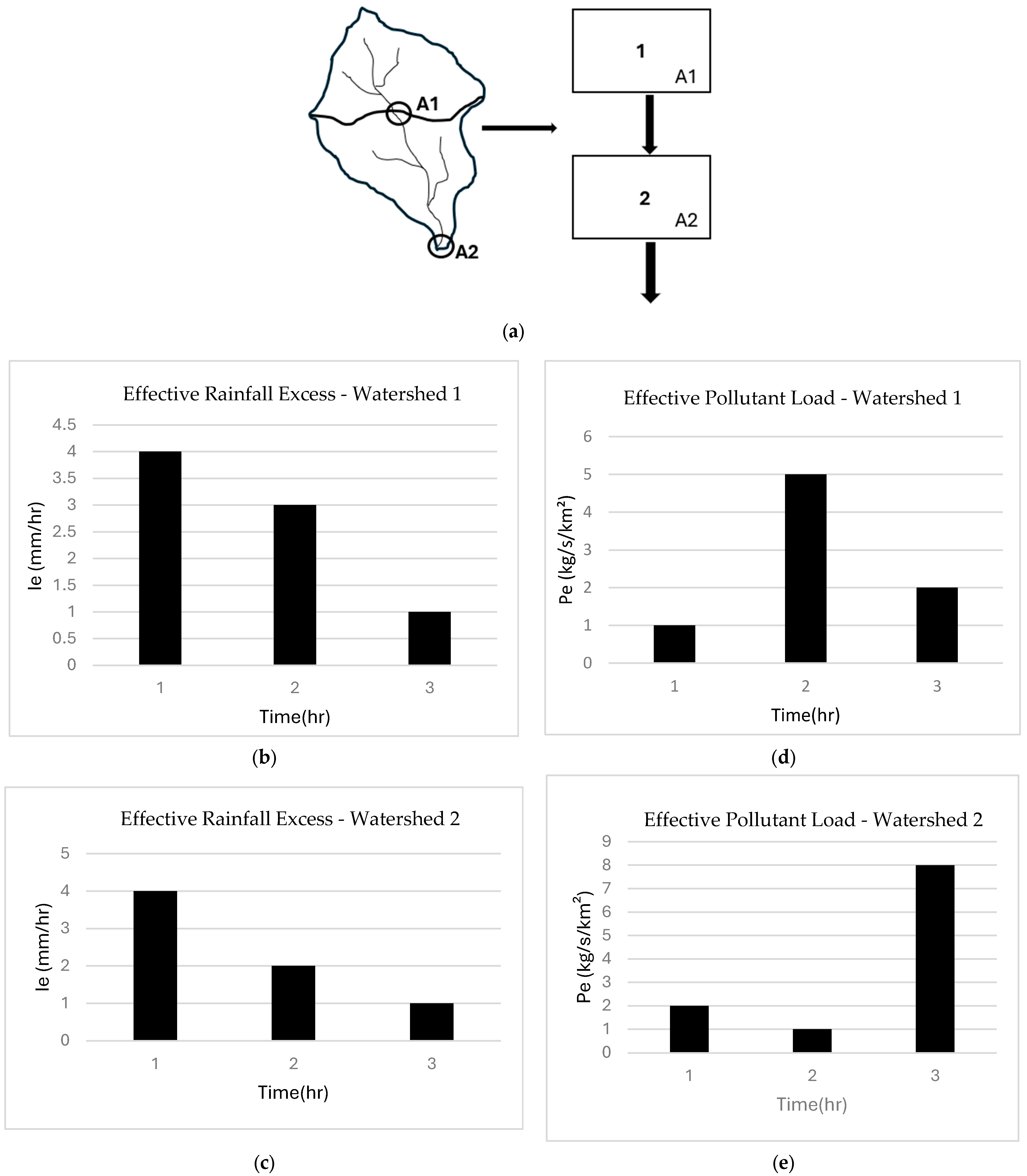
This example shows a two-cell watershed (Figure 3) in which each cell acts as a separate hydrological unit, while surface runoff connects them. This setup reflects how real-world watersheds operate, with upstream regions influencing downstream areas through the movement of water and pollutants.

The model distinguishes between direct and indirect rainfall input. Direct rainfall refers to precipitation falling directly onto a watershed cell, contributing immediately to effective rainfall excess and surface runoff. Indirect rainfall, or transferred runoff, occurs when runoff from one cell moves downstream into another. This distinction is critical in the two-cell watershed case, where runoff from Watershed 1 contributes additional water input to Watershed 2 beyond direct precipitation.

In Watershed 1, the effective rainfall intensity varies over time due to land characteristics such as soil permeability and vegetation cover. While some rainfall infiltrates or evaporates, a significant portion generates surface runoff, as shown in Figure 3b. The hydrograph response (Figure 4a) exhibits a rapid increase in flow rate followed by a gradual decline, reflecting the transformation of effective rainfall into runoff. Pollutant transport follows a similar pattern, with peak concentrations occurring at the early stages of runoff generation (Figure 4b). Instead of being retained, most runoff and pollutants from Watershed 1 are transported downstream, contributing to Watershed 2’s hydrological and water quality responses.

Watershed 2 receives runoff from both direct precipitation and inflow from Watershed 1, leading to higher effective rainfall intensity (Figure 3d). Consequently, peak discharge is more pronounced due to the combined immediate response to local rainfall and the delayed contribution from upstream runoff (Figure 3e). The flow rate at the outlet (Figure 4c) surpasses that of Watershed 1, with a later peak reflecting the cumulative effect of both rainfall components. The pollutant concentration at the outlet (Figure 4d) also exhibits a higher peak due to pollutant transport from Watershed 1, amplifying contamination downstream.

Mass balance analysis confirms that the total input to Watershed 2 comprises direct rainfall (calculated as $I_e\times t\times A_2$) and indirect runoff from Watershed 1, computed using the Diskin kernel function. The model conserves mass, ensuring that the total inflows and outflows align, with minor discrepancies attributed to numerical approximations. A similar process transports pollutants, carrying contaminants from Watershed 1 into Watershed 2. Consequently, pollution control in Watershed 2 must address not only local contamination but also upstream pollutant contributions. High pollutant loads in Watershed 1, whether from industrial discharge, agricultural runoff, or urbanization, directly impact downstream water quality, reinforcing the importance of integrated watershed management strategies.

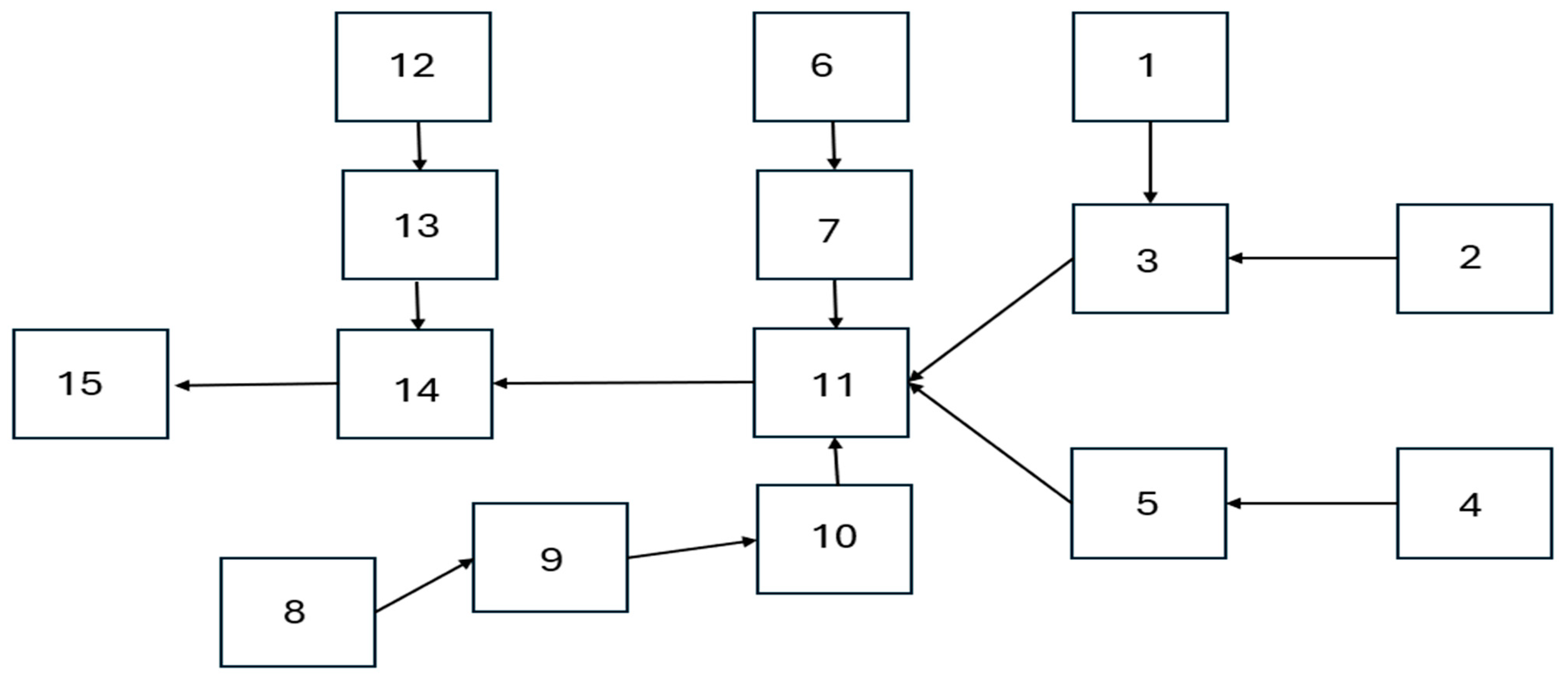
3.3. Fifteen-Cell (Bellebeek) Watershed

This example represents a 15-cell watershed, shown in Figure 5, extending the principles demonstrated in the 2-cell example extracted from Diskin’s pioneer work [4]. Unlike the simpler case, where only two interconnected units controlled flow and pollutant transport, this model captures a more complex watershed structure with multiple contributing sub-watersheds. Each cell in the system functions as an independent hydrological unit, receiving direct rainfall excess—contributing to local runoff; runoff from upstream cells—adding additional flow and pollutants from contributing areas; and flow routing through a connected network—ultimately leading to pollutant transport downstream.

All parameters used in this example were derived from Diskin’s paper [4]. The reservoir routing coefficient was set to KA = 3.73 [h], the linear channel length constant to DA = 0 [h], and the channel routing coefficient to TA = 1.31 [h]. Since not all cell areas and channel lengths were provided in Diskin’s paper, a full list of cell areas and channel lengths can be found in Table 1.

The 15-cell watershed model extends the principles of rainfall–runoff and pollutant transport analysis by incorporating a hierarchical structure of interconnected sub-watersheds. The results from this model highlight key mass conservation properties and the influence of watershed topology on flow and pollutant transport. This conservation is observed across individual cells and the watershed, maintaining a balance between inflows and outflows.

A key observation in this model is that sub-watersheds 1 and 2 exhibit identical flow rates and pollutant concentrations at their outlets (Figure 6 and Figure 7). The figures illustrate the flow rate and pollutant concentration over time for Cell 1 and Cell 2, respectively, demonstrating their identical hydrological responses. The flow rate in both cells follows a characteristic hydrograph pattern, with a rapid increase due to rainfall input, a peak discharge at around 5 h, and a gradual decline to near zero by 30 h. Similarly, the pollutant concentration exhibits a rising and falling trend over time. The identical trends observed in both cells confirm that their behavior is entirely dictated by local rainfall and pollutant mobilization, as no upstream inflows contribute additional water or pollutants. Given that both watersheds have the same morphological characteristics and precipitation inputs, their runoff and pollutant transport remain consistent. This demonstrates the principle of mass conservation, where the total pollutant load mobilized by rainfall is proportionally reflected in the watershed outlet.

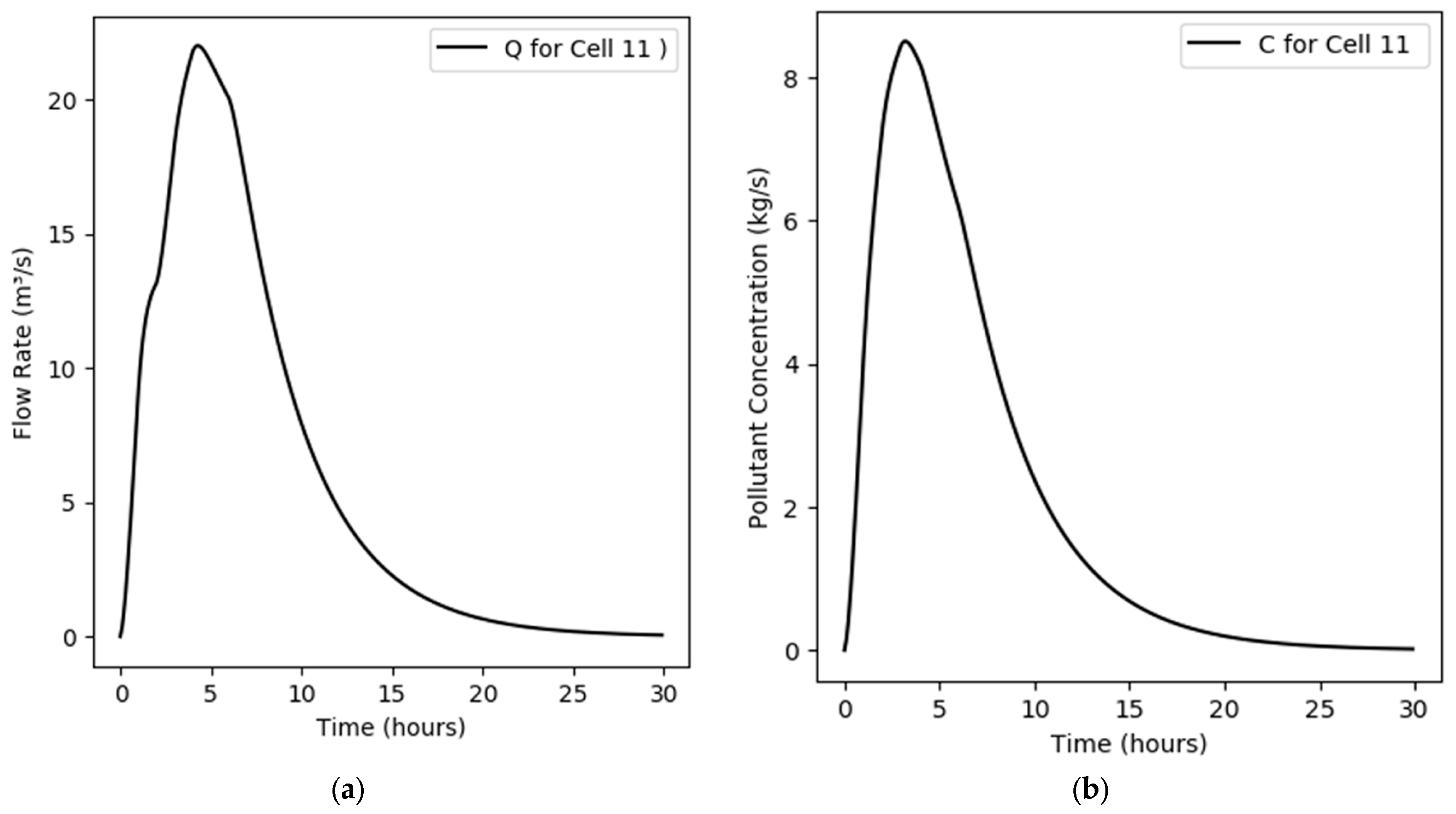
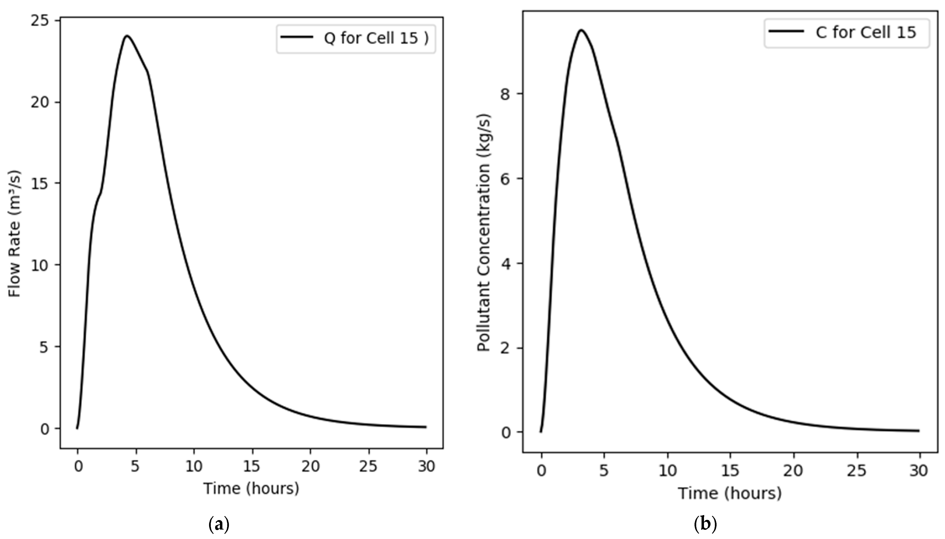
A more complex case is observed between Cell 11 and Cell 15, as illustrated in Figure 8 and Figure 9. The graphs show that both the flow rate (Q) and pollutant concentration (C) in Cell 11 and Cell 15 exhibit nearly identical trends, confirming the role of Cell 11 as a major contributor to the watershed outlet. Unlike Watersheds 1 and 2, where the similarity in flow and concentration arises due to their isolated nature, the resemblance between Cell 11 and Cell 15 is a direct result of hydrological accumulation and mass transport dynamics.

As seen in Figure 8, Cell 11 receives substantial inflows from multiple upstream cells, making it a key node in the watershed’s hydrological and pollutant transport processes. This results in a high peak flow rate and pollutant concentration, which are then passed downstream to Cell 15, the watershed outlet. The graphs in Figure 9 confirm that the flow rate and pollutant concentration at Cell 15 closely follow those of Cell 11, with only minor dilution effects from lateral inflows or potential retention along the channel pathway.

The near identical profiles of Cell 11 and Cell 15 further validate the principle of mass conservation, as the pollutant load transported by runoff in Cell 11 is largely preserved as it moves toward Cell 15. This emphasizes the importance of monitoring and managing key nodes like Cell 11, as changes in its pollutant dynamics will have a direct impact on the overall water quality at the watershed outlet.

While the simulation results confirm the model’s structural integrity and its ability to represent flow and pollutant propagation, uncalibrated scenarios may not fully align with observed pollutant concentrations. To enhance predictive accuracy and preserve mass consistency, the model undergoes a structured calibration process. The subsequent section presents this calibration approach and evaluates its impact on model performance.

4. Calibration

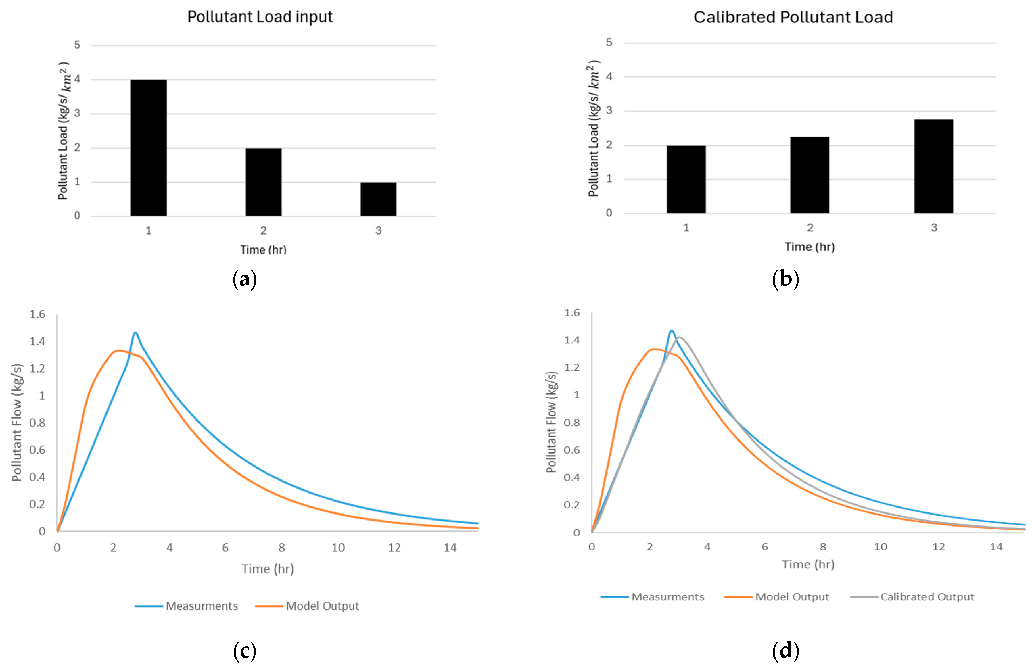
The calibration process in our model was performed using a scaling factor (α) applied to the pollutant load histogram. This factor was designed to adjust the input pollutant concentrations while ensuring that the total mass of pollutants remains conserved. The goal of this calibration was to minimize the discrepancy between the modeled pollutant concentration at the watershed outlet and the measured pollutant concentration from observed data. As illustrated in Figure 10, the initial pollutant input distribution (Figure 10a) had varying values across different time steps. However, when using the uncalibrated model (Figure 10b), the pollutant concentration at the outlet deviated from the measured data, as seen in the comparison between the measured pollutant flow (blue curve) and the model output (orange curve) (Figure 10c). To correct this, a set of scaling factors (${\alpha }_i$, ${\alpha }_{i+1}$, …, ${\alpha }_n$), where $i$ is the time step, was introduced, where each α value adjusts the corresponding time step in the pollutant load histogram. This adjustment ensured that the shape of the pollutant concentration curve from the model aligned more closely with the observed data while still preserving the total pollutant mass.

Mathematically, the calibration process involved optimizing F(x), which represents the difference between the measured and simulated pollutant concentrations. The α values were chosen such that F(x) was minimized, effectively shifting the input pollutant distribution to compensate for errors in the model’s initial prediction. The result of this calibration is visible in the final output, where the calibrated pollutant flow (gray curve) now closely follows the measured data. This approach provides a data-driven correction to the pollutant transport model while maintaining mass balance, ensuring that no artificial loss or gain of pollutants occur.

To extend the mathematical formulation, we can further analyze the pollutant transport system using a system analysis approach. By defining the governing equations explicitly, we can explore the sensitivity of the model to variations in α, assess the stability of the calibration process, and quantify uncertainty in pollutant transport predictions. Additionally, incorporating constraints ensures that the calibrated model adheres to physical conservation laws, maintaining consistency between the input pollutant loads and the observed flow. This structured approach enhances the robustness of the calibration process, providing a more reliable representation of pollutant dynamics.

$$Min F(x) ={\sum }_{i=1}^n(P-{P\prime )}^2$$

(15)

$$\begin{gathered} Subjected to: \sum p{l}_i=\sum {\alpha }_i\cdot p{l}_i,\forall i \\ {\alpha }_i\le 10 \\ {\alpha }_i\ge 0.01 \end{gathered}$$

(16)

4.1. Single-Cell Calibration

The single-cell calibration process aims to optimize the model’s ability to predict both hydrological responses (flow rate) and pollutant transport dynamics at a basic watershed level. This step is critical, as it serves as the foundation for more complex multi-cell watershed simulations.

In this example, the initial conditions were set based on the single-cell watershed from Section 3.1. (Figure 2) with an area of 5.92 km², with the same rainfall input and pollutant load distribution over three time intervals. The Python script used for calibration defines key model parameters, such as the reservoir coefficient (KA), lag time (DA), and transport coefficient (TA), which influence runoff generation and pollutant dispersion. The pollutant input distribution (as shown in Figure 10a) was initially unbalanced, causing discrepancies between the measured pollutant concentration (red curve) and the uncalibrated model output (blue curve) (Figure 10c).

To correct this, a scaling factor (α) was introduced for each pollutant input time step. The scaling coefficients (α₁, α₂, α₃) were optimized to adjust the pollutant input while ensuring mass conservation, meaning that the total pollutant mass before and after calibration remained constant. The corrected pollutant load (as shown in Figure 10b) resulted in a better alignment between the model’s output and observed measurements, significantly reducing the error in concentration predictions.

Figure 10d shows how the corrected output (green curve) closely follows the measured pollutant concentration (red curve), indicating that the calibration successfully improved the model’s accuracy. This method ensures that the model correctly represents the timing and magnitude of pollutant peaks, which is essential for accurate water quality modeling and watershed management. In the calibration process, the scaling factors (α₁, α₂, α₃) were introduced to adjust the pollutant load input while ensuring that the total mass of pollutants remained unchanged. The values of the scaling factors were optimized as α₁ = 0.505, α₂ = 1.101, and α₃ = 2.737, meaning that the first time step’s pollutant input was reduced, while the later time steps’ inputs were increased, as shown in Figure 11. This adjustment redistributed the pollutant load over time to improve the alignment between the simulated and measured pollutant concentrations at the watershed outlet, as seen in Figure 12b. To ensure mass conservation, the total pollutant mass before and after calibration was calculated using Equation (13), and obtaining that after calibration, the pollutant load values were modified, but the total mass remained constant. This ensures that while the distribution of pollutants was adjusted, the total amount of pollutants transported through the system was conserved. The redistribution helped reduce discrepancies between the measured and modeled pollutant concentrations, improving the accuracy of the watershed simulation while adhering to mass conservation principles.

4.2. Two-Cell Calibration

The calibration process for the two-cell watershed aims to refine pollutant transport predictions by adjusting the input pollutant loads to match observed data. Given the interconnected nature of the two-cell system, errors in upstream pollutant estimates propagate downstream, necessitating a sequential calibration approach.

The calibration of Cell 1 in the two-cell watershed model focused on adjusting the pollutant load distribution while ensuring that mass conservation was maintained. Before calibration, the pollutant load (Figure 12a) was unevenly distributed across time steps, with the second time step (t = 2 h) having a significantly higher input. This discrepancy resulted in a modeled pollutant concentration (blue curve in Figure 12c) that was overestimated compared to the measured data (red curve in Figure 12c), indicating that the model was not accurately capturing the pollutant transport dynamics.

To correct this, scaling factors (α₁, α₂, α₃) = (1.126, 0.768, 1.016) were applied, adjusting the pollutant input at each time step. This process redistributed the pollutant load while ensuring that the total mass of the pollutant remained constant. The effect of this adjustment is visible in Figure 12b, where the recalibrated pollutant load shows a more balanced distribution across time steps. The impact of calibration on the pollutant concentration is illustrated in the corrected output graph (Figure 12d), where the green curve (calibrated model output) now closely follows the measured data (red curve). The peak concentration has been reduced and shifted, bringing the model’s predictions in line with observed pollutant transport behavior.

Since Cell 2 receives contributions from both direct rainfall and upstream inputs from Cell 1, its calibration was more complex. Initially, the model overestimated the pollutant concentration in Cell 2, as seen in the large deviation between the measured data (red curve) and the uncalibrated model output (blue curve) in Figure 13c,d. This discrepancy was primarily due to an incorrect pollutant load distribution, where most of the pollutant input was concentrated in the third time step (Figure 13a). To correct this, optimized scaling factors (α₁, α₂, α₃) = (0.699, 4.403, 0.65) were applied, leading to a more balanced pollutant input distribution (Figure 13b). After calibration, the corrected output (green curve in Figure 13d) closely matched the observed pollutant concentration, with both the peak timing and magnitude accurately represented.

The calibration of Cell 1 directly influenced Cell 2, as pollutants from Cell 1 flow into Cell 2. By first correcting the upstream pollutant transport, the pollutant concentration in Cell 2 became more accurate, ensuring that the model correctly captured pollutant accumulation and downstream transport dynamics. The results confirm that after calibration, the modeled pollutant concentrations in both cells closely match the observed data, improving the model’s predictive capabilities.

This calibration approach highlights the importance of considering upstream–downstream interactions in watershed models. Errors in upstream cells can propagate through the system, making stepwise calibration essential for achieving accurate results in multi-cell models. These findings provide a strong foundation for applying the model to larger and more complex watershed systems, such as the 15-cell model, where multiple sub-watersheds interact to influence pollutant transport at the watershed outlet, as will be shown in the next section.

4.3. Fifteen-Cell (Bellebeek Watershed) Calibration

The calibration process for the 15-cell watershed model was more intricate than the previous single- and two-cell cases, requiring adjustments across multiple interacting sub-watersheds. This time, a 0.25 h time step was used, with the same pollutant load event in each cell (Figure 14) allowing finer temporal resolution in pollutant transport dynamics. The goal was to refine the model’s accuracy by determining the optimal α scaling factors for each cell that minimize the discrepancy between simulated and measured pollutant concentrations while ensuring that mass conservation principles remain intact.

Using a 0.25 h time step improved the model’s ability to capture rapid changes in pollutant dynamics, especially in the early phases of runoff generation. This finer resolution allowed for more precise tuning of the α values, leading to a smoother, more physically realistic representation of pollutant transport across the watershed. The improved time resolution also helped in capturing short-duration peak concentrations, which would have been smoothed out with a larger time step.

Before calibration, the pollutant load distribution was inconsistent, with an overrepresentation in the initial time steps, leading to overestimated peak pollutant concentrations in the model. Figure 14 shows the pollutant load input before calibration, with high values in the early hours, which caused discrepancies between the simulated and observed concentration curves at various watershed nodes. To correct this, a set of 12 optimized α scaling factors, for each time step in a 3 h storm event, were applied across time steps, effectively redistributing the pollutant load.

The impact of calibration is evident when analyzing the corrected pollutant concentration curves for key cells such as Cell 1, Cell 2, and Cell 15—the watershed outlet. Initially, the model overpredicted peak pollutant concentrations in most cells, with the model output curves showing significantly higher peaks than the measured values curves. After calibration, the corrected output curves align closely with observed data, indicating that the model is now better representing real-world pollutant transport behavior.

The calibrated pollutant load shown in (Figure 15) demonstrates a smoother, more evenly distributed pollutant input, leading to a more realistic pollutant concentration profile at key locations within the watershed. Cells 1 and 2 were particularly critical because they share the same morphological and hydrological characteristics, leading to identical pollutant concentration patterns (Figure 16).

However, Cell 15, located at the watershed outlet, required more careful tuning since it accumulates runoff and pollutants from all upstream cells. The calibration process ensured that the final pollutant load reaching the outlet reflected contributions from all upstream sources accurately, avoiding artificial dilution or concentration spikes (Figure 17).

5. Discussion

The results confirm that the adapted Diskin Cell Model effectively simulates both the hydrological response and pollutant transport across watershed systems of increasing complexity. In the single-cell case (Figure 2), the model reproduces typical runoff behavior and pollutant concentration trends, with mass conservation maintained through alignment of input rainfall and output flow volumes. The pollutant hydrograph closely mirrors the flow response, demonstrating the utility of the convolution approach in linking rainfall-driven mobilization to downstream pollutant dynamics.

In the two-cell system (Figure 3 and Figure 4), the influence of upstream contributions becomes evident. Watershed 1 generates flow and pollutants that are subsequently routed into Watershed 2, amplifying its hydrological and pollutant responses. The increases in peak discharge and pollutant concentration in Watershed 2 (Figure 4c,d), relative to Watershed 1 (Figure 4a,b), illustrate the importance of accounting for both direct and indirect inputs in pollutant transport models.

The 15-cell Bellebeek watershed benchmark example (Figure 5, Figure 6, Figure 7, Figure 8 and Figure 9) highlights the model’s scalability and internal consistency. Cells with identical morphology and inputs (Cells 1 and 2) yield nearly identical flow and pollutant profiles (Figure 6 and Figure 7), validating spatial coherence. Meanwhile, the close similarity between Cell 11 and the outlet Cell 15 (Figure 8 and Figure 9) demonstrates pollutant accumulation from upstream sources and confirms the importance of internal nodes in controlling downstream water quality.

Model calibration significantly improved pollutant concentration predictions while preserving mass conservation. In the single-cell case, time-step-specific scaling factors ($\alpha$) were applied to the pollutant input (Figure 11a–b), resulting in a closer match between modeled and observed concentrations (Figure 11d). We achieved similar improvements in the two-cell system (Figure 13). In the 15-cell case, the use of finer time steps and calibrated pollutant loads (Figure 14 and Figure 15) yielded improved alignment between simulated and measured concentrations at key locations (Figure 16, Figure 17 and Figure 18), particularly at the watershed outlet.

However, we acknowledge that this calibration method does not incorporate stochastic variability or formal uncertainty quantification. Future enhancements may include Monte Carlo simulation or Bayesian inference techniques to assess model sensitivity and robustness under real-world heterogeneous conditions.

Assumptions and Limitations:

This study is based on several assumptions that simplify the complex processes involved in rainfall–runoff and pollutant transport modeling. First, the model assumes that the watershed is already contaminated; rainfall-driven surface runoff triggers prior to the rainfall event, solely. Processes such as pollutant generation during the event, sediment–pollutant interactions, and in-stream chemical transformations are not explicitly modeled.

The pollutant transport mechanism relies on convolution with the Instantaneous Unit Hydrograph (IUH), assuming linear and time-invariant behavior of pollutant routing across cells. This implies that pollutant dispersion is proportional to the runoff response, without accounting for adsorption, decay, or biological degradation. Furthermore, the effective pollutant load is assumed to be a fixed fraction of the total available load, modifiable through calibration scaling factors rather than being dynamically linked to rainfall intensity, land use, or soil properties.

The model also assumes homogeneity within each cell and uniformity in the hydrological response for morphologically identical cells. This can limit accuracy in heterogeneous catchments with significant land use variation, complex topography, or subsurface flow contributions.

In terms of data, the model relies on calibrated pollutant load inputs and observed outlet concentrations for validation. Limited data or the absence of high-resolution pollutant data in some watersheds can impair model performance and transferability. Additionally, while calibration preserves mass conservation, it does not guarantee the uniqueness of the solution, and results may be sensitive to the choice and distribution of scaling factors.

Due to the model’s uniqueness and the lack of extensive studies focusing on pollutant mobilization under similar assumptions and constraints (i.e., no dynamic pollutant decay, no sediment interactions, and limited water quality inputs), we currently cannot provide direct comparisons with other models or their results. Benchmarking the model against established tools like SWMM, SWAT [11], QUAL2K [16], or HSPF is an important future direction but is out of the current scope, given the fundamental differences in model structure, data requirements, and objectives.

As a result, we have validated the model through comparison with observed and simulated effluent concentrations across different watershed complexities (1-cell, 2-cell, 15-cell configurations), demonstrating its internal consistency, scalability, and ability to preserve mass conservation.

Even though the model does not currently include sensitivity or uncertainty analyses, nor detailed pollutant fate mechanisms, its simplicity and flexibility offer a practical event-based tool.

It captures spatial and temporal pollutant dynamics effectively and identifies critical cells that govern downstream pollution, providing valuable guidance for monitoring and management strategies.

6. Conclusions

This study advanced Diskin’s Instantaneous Unit Hydrograph (IUH) framework to model pollutant transport in rainfall–runoff systems, integrating it with Diskin’s Cell Model to ensure mass conservation and accurate pollutant load predictions. By maintaining a uniform hydrological response across watershed cells, the model effectively simulated pollutant routing while preserving computational efficiency.

The model treated pollutants as surface-bound inputs, estimating the fraction reaching the outlet without explicitly modeling decay processes. Instead, it utilized pollutant distribution data and field measurements to calibrate transport dynamics. Single-cell, two-cell, and fifteen-cell calibrations refined pollutant input scaling, aligning predictions with observed concentrations. The pollutant hydrograph at each cell adhered to a consistent IUH-based transport function, ensuring systematic dispersion. In the 15-cell case, a 0.25 h time step enhanced the resolution of short-duration transport events, crucial for stormwater pollution modeling. Results underscored the cumulative impact of upstream pollutant contributions on downstream water quality, reinforcing the necessity of targeted watershed management.

This approach offers a structured and scalable solution for hydrological and environmental applications, including stormwater quality control and pollution mitigation. However, the model simplifies transport processes, requiring extensive calibration while omitting finer-scale pollutant interactions. The model’s lack of sediment transportation can be seen as a limitation. Future research should incorporate sediment dynamics, adsorption mechanisms, and real-time data assimilation to refine predictive accuracy and broaden applicability.