Quantifying Baseflow Changes Due to Irrigation Expansion Using SWAT+gwflow

Abstract

Baseflow, the portion of streamflow sustained by groundwater discharge, is crucial for maintaining river ecosystems. Irrigation practices could influence baseflow, with varying impacts depending on the irrigation practices. This study evaluates the impact of irrigation expansion on baseflows, accounting for weather-driven irrigation demand. The SWAT+gwflow model was applied to the San Antonio Catchment (225 km²) in Uruguay, a region dominated by intensive horticulture and citrus farming reliant on groundwater. Irrigation expansion involves extending irrigated areas from 6193 to 8561 hectares, increasing average groundwater use by 18.4%. Model projections over 25 years indicate up to 1.2 m of annual groundwater depletion, including severe local reductions in monthly baseflow during dry years. Limitations have been discussed and compared with applications in other regions. These results have implications for water management, as current regulations ignore groundwater–surface water interactions and fail to account for variable irrigation water demand in high variable weather conditions. This approach provides a tool to anticipate the environmental effects of irrigation expansion and supports the development of adaptive regulations that better align with hydrological realities.

1. Introduction

In hydrology, baseflow refer to the portion of streamflow sustained by groundwater seepage during dry periods [1], plays a critical role in maintaining ecological balance and supporting water-dependent activities. However, groundwater extractions for irrigated agriculture can deplete aquifers and reduce baseflow, potentially impacting ecosystems and downstream users [2,3,4,5]. While modern irrigation systems improve efficiency, they may paradoxically encourage the expansion of irrigated areas, leading to unintended consequences for water [6,7,8,9,10,11]. Therefore, understanding the interactions between groundwater, irrigation, and baseflow is key for sustainable water management [12].

Climate variability is a major driver of yield fluctuations globally, accounting for around one-third of observed variation [13]. In this context, supplementary irrigation offers farmers a way to stabilize yields and reduce losses in dry years [14,15]. Irrigation schedules are typically adjusted based on crop needs, weather, and soil moisture conditions [16,17], meaning that water use fluctuates annually even when crop types and irrigated areas remain constant [18]. However, water permits are often granted based on fixed annual requirements, rarely accounting for seasonal or inter-annual variability in demand [19,20]. This disconnect limits the effectiveness of regulation, which is often poorly equipped to address the dynamic nature of real-world water use, potentially masking the cumulative impacts of variable irrigation on baseflows.

These challenges are especially pronounced in groundwater-fed irrigation systems, where dynamic feedbacks between surface water, groundwater, and irrigation demands are difficult to quantify [21]. Understanding these dynamics is essential for developing sustainable irrigation strategies [22]. Here, hydrological models provide valuable tools for exploring such interactions and supporting decision-making [23,24].

The SWAT model (Soil and Water Assessment Tool) [25] has been widely used to simulate agricultural catchments, including hydrological processes and water management [26,27,28,29,30]. Enhanced versions of SWAT have aimed to better represent groundwater and surface water exchanges (GW-SW). Among them, SWAT+gwflow [31] provides an improved, two-dimensional simulation of groundwater, capturing vertical (e.g., evapotranspiration, percolation, infiltration, exfiltration, pumping) and horizontal (e.g., later flows) water movements, and has been successfully applied in a wide range of studies [32,33,34,35,36]. Compared to SWAT+standalone [37], which represent vertical flow, SWAT+gwflow offers a better compromise between process realism and usability, making it well suited to the objectives of this work. Although SWAT-MODFLOW [38] enables full 3D simulation and multi-layer aquifer representation [39,40], its high data requirements and computational costs limit its applicability.

This study focuses on the San Antonio catchment in northern Uruguay, an area dominated by intensive, groundwater-irrigated horticulture and citriculture [41,42]. Its high density of hydrometeorological data and sensitivity to El Niño–Southern Oscillation (ENSO)-driven climate variability [43] make it an ideal setting to investigate irrigation–groundwater–streamflow interactions. Increasing reliance on groundwater during dry years intensifies pressure on water resources [44], raising concerns about long-term impacts on baseflow.

This study aims to evaluate how irrigation expansion affects baseflows under inter-annual weather variability. It hypothesizes that increased summer groundwater extraction reduces baseflow during the irrigation season, with the magnitude of this impact varying spatially across the catchment according to the degree of hydraulic connectivity between the aquifer and the stream. These effects are further influenced by climatic conditions, with more pronounced reductions in baseflow during dry periods. While climate change is not explicitly modeled, climate variability is treated as a key driver of irrigation dynamics and constraints.

2. Materials and Methods

This study establishes a groundwater–surface water modeling framework for the San Antonio catchment, located in northern Uruguay, an area characterized by a humid subtropical climate and intensive agricultural activity. The methodological approach combines field observations, farmer interviews, and global datasets to support the calibration and validation of a SWAT+gwflow model, capable of explicitly representing surface and subsurface hydrological processes.

Section 2.1 describes the study area, the monitoring network, and the available datasets. Section 2.2 details the model setup, including subbasins, stream channels, and the aquifer. The model calibration was conducted in two phases: an initial calibration focused on streamflow using observed discharge data, followed by a second phase aimed at minimizing errors in simulated groundwater heads and baseflow using groundwater level observations. Land use and agricultural management practices were characterized through field surveys and interviews to accurately incorporate typical crops, irrigation schedules, and water allocation to set up the model. Section 2.3 presents the theory for the quantification of uncertainties and goodness-of-fit metrics (GoF).

Section 2.4 outlines the assumptions made regarding groundwater pumping and irrigation expansion. The potential impacts of expanding irrigation in rainfed citriculture areas were evaluated over a 30-year historical period. Climate variability was accounted for by classifying months as wet, normal, or dry based on precipitation percentiles, enabling a detailed analysis of water use dynamics under different climatic scenarios.

All the figures in this work were generated in R. The R scripts are available in the PDF file in the supplementary material. The tool developed in this work is open and can be downloaded from the Open Science Framework (OSF) repository of the project [45].

2.1. Study Area and Dataset

The San Antonio Catchment covers an area of 225 km² and experiences a humid subtropical climate, as classified by the Köppen climate system [46]. The mean annual rainfall is 1430 mm, with lower monthly precipitation during the winter months (June, July, and August). Average daily temperatures range from 10 to 15 °C in winter and from 20 to 30 °C in summer [41]. The monitoring network, maintained by the “Departamento del Agua—CENUR Litoral Norte” since 2018, includes eight observation wells for groundwater, one hydrometric station with reliable discharge computations for surface water (Figure 1c), and fourteen rain gauges distributed throughout the region.

The land use within the catchment (Figure 1a) is characterized by a significant proportion of open field horticulture (OFCP, 34.7%) and citriculture (ORAN, 20.3%), both of which rely on a combination of rainfed crops and irrigation [47]. Most of the irrigation zones are in the southwest of the catchment, while the northern area holds potential for developing supplementary irrigation, particularly for citrus crops (Figure 1b). In addition, the catchment features a large proportion of grassland (GRAS, 35.6%) and pastures (PAST, 0.6%), both utilized for grazing livestock. Other minor land uses include forestry plantations (EUCA, 1.6%), native forest (FRSE, 4.2%), greenhouse horticulture (GHCP, 0.8%), summer crops (AGRL, 2.1%), and urban areas (URBN, 0.1%). Cross-slope tillage is predominant in OFCP. The use of residue cover under conventional tillage is common in OFCP and AGRL, while GRAS typically lacks residue cover. Heavy forest cover and shortgrass are typical for EUCA, FRSE, and ORAN. This diverse land use pattern reflects the multifunctional nature of the catchment.

The terrain is relatively flat, characterized by a rolling landscape with occasional small hills (Figure 1c). Groundwater heads at steady state range from 20 to 80 m (Figure 1d). Steady state refers to an assumption in which all groundwater fluxes remain constant over time, with no change in groundwater storage and inflows equal to outflows. This assumption can be used in simplified models, for long-term average conditions, or for initializing transient models such as SWAT+gwflow. The present study uses previously estimated steady state conditions from MODFLOW for the year 2019 as initial conditions [44]. However, since a warm-up period is included, any potential bias introduced by these initial conditions is expected to be minimized. Elevation is referenced from the official datum of Uruguay, which corresponds to the mean water level of Río de la Plata (River Plate) at the port of Montevideo. The upper catchment is dominated by silty clay-textured Haplic Vertisols (50–60% clay, 28–42% silt, 9–12% sand). These soils have high cation exchange capacity (CEC), elevated base saturation, and near-neutral pH, contributing to their natural fertility. Their fine texture and expansive clays enhance water and nutrient retention but also reduce infiltration under saturated conditions, increasing the risk of waterlogging. In contrast, the lower catchment is mainly composed of Luvic Phaeozems with a humic phase. These soils are acidic, with low base saturation, reduced CEC, and a sandy surface horizon that transitions abruptly to a clay-rich subsoil (6–36% clay, 7–11% silt, 56–87% sand). This profile limits moisture retention. While moderate organic matter may mitigate some constraints, these soils are prone to nutrient leaching and have low water-holding capacity [48].

Geology comprises sedimentary deposits and fissured basalt rocks from the Cretaceous–Tertiary periods, which form part of the Salto–Arapey aquifer [42,49]. The Global hydrogeology maps (GLHYMPS) of the permeability dataset [50] identifies four zones with distinctive aquifer hydraulic conductivities (Figure 1e). Fractured volcanic (effusive) rocks from the Mesozoic, primarily of Jurassic to Cretaceous age, predominate in the geology of the region (Figure 1e, green) and correspond to the Salto–Arapey Formation [42]. Alluvial and fluvial deposits from the Cenozoic Pliocene are shown in Figure 1e (red), while fluvial deposits from the Cenozoic Holocene are shown in Figure 1e (blue). A thinner transition zone (Figure 1e, yellow) is also identified by GLHYMPS. This zone has not been associated with any known geological formation and exemplifies the heterogeneity and complexity of the geological structures in this small area. Its relatively limited extent and distinct pattern suggests that it may represent a transition to fractured basalt from a less permeable unit. Additionally, SoilGrids data [51] indicates an absolute depth to bedrock (aquifer thickness) ranging from 10 to 40 m (Figure 1f).

2.2. Groundwater–Surface Water Model

SWAT+gwflow [31] is an extension of the SWAT+ model [37] that integrates a computationally efficient, 2D finite-difference groundwater flow model to enhance the simulation of GW-SW. This extension provides a more explicit representation of groundwater flow dynamics at a reasonable computation cost. In the model, surface water processes are represented through hydrologic response units (HRUs), which are polygons defined by the combination of land use, soil type, and slope. HRUs serve as the primary elements for hydrological production functions, such as infiltration, exfiltration, and surface runoff. Their structure remains consistent with the SWAT+standalone model. The model’s transfer function—governing surface and subsurface routing as well as storage—is defined by channels and an aquifer grid. Each aquifer grid cell is linked to its corresponding HRU polygons through spatial overlap. The proportion of each HRU that falls within a grid cell, relative to its total area, is used to compute GW-SW and to calculate a partial recharge volume from a single HRU to the grid cell. As several HRUs can overlap a grid cell, the total recharge volume from HRUs is estimated by summing all partial recharge contributions. Stream cells are also identified by intersecting the stream network with the gwflow grid. This methodology follows the guidelines outlined in the gwflow tutorial [52]. These features allow for the representation of spatial variability in aquifer recharge (derived from SWAT+) and aquifer outflows (e.g., groundwater pumping or discharge to channels).

The change in groundwater storage (∆S) is calculated as the difference between all inflows and outflows, as water depth in millimeters, calculated with respect to the entire basin area (1).

∆S = rech + swgw − gwet − gwsw − satx − soil − ppag ± latl ± bndr

(1)

Inflows (positive values, indicating water added to an aquifer grid cell) include soil water percolating to groundwater (rech) and stream seepage to groundwater (swgw). Outflows (negative values, indicating water removed from an aquifer grid cell) include groundwater lost through evapotranspiration (gwet), discharge to streams (gwsw), saturation excess flow (satx), upward transfer to the soil zone (soil), and pumping for agricultural irrigation (ppag). Bidirectional fluxes (positive or negative values, indicating water added to or removed from an aquifer grid cell) include lateral groundwater flow between cells (latl) and boundary fluxes at the watershed edge (bndr). These outputs are stored in the groundwater balance files. Other types of files generated by the model include groundwater raster files, with fluxes in m³/day, and water balance files at the HRU scale, with fluxes calculated as water depth in millimeters relative to the HRU area.

The San Antonio catchment is modelled with 411 HRUs, ranging in size from 0.1 to 2200 hectares; 37 channels, varying in length from 70 to 9000 m; 24 subbasins, spanning from 0.22 to 31 km²; and an aquifer grid comprising 161 by 284 cells, each with a resolution of 100 by 100 m. Precipitation from local rain gauges was pre-processed using inverse distance interpolation. This interpolation represents the average precipitation for each sub-catchment, which serves as the precipitation input for the model. Agricultural management practices, including crop types, planting and harvesting schedules, fertilization, and irrigation strategies, were identified through interviews with local farmers. This information was then incorporated into the model to reflect the dominant land uses across the catchment. Irrigation pumping rates were set based on the water demands of irrigated crops, ensuring that simulated water usage aligns with real-world agricultural requirements. Key aquifer properties, such as aquifer thickness and hydraulic conductivity, were defined using global datasets (Figure 1e,f). Boundary conditions were assumed to have constant hydraulic heads, enabling groundwater exchange with adjacent catchments.

The model was calibrated during the period from 1 February 2019 to 1 August 2021. Results were validated for the periods from 8 August 2018 to 1 February 2019 and 1 September 2021 to 5 February 2021. A four-year warm-up period was applied prior to the calibration/validation phase. These calibration and validation windows were selected to ensure the occurrence of dry and wet periods, with the calibration window comprising two-thirds of the total period of available data. For that purpose, a two-phase supervised random calibration process was used. This process involves a series of iterations, beginning with a uniform distribution across specified parameter ranges. In each iteration, the model runs 360 times, and each simulation is evaluated using the objective function specific to the corresponding calibration phase. The first phase prioritized achieving the best possible fit for streamflow simulations, assessed using the Kling–Gupta Efficiency (KGE) metric [53], as it has been proven to be a good criterion for model calibration [54]. The model parameters calibrated during this phase are listed in

Table 1. Calibration parameter for the 1st phase (total streamflow).

Parameter	Description	File	Range	Type of Change	Best Fit
cn	Curve number compensation factor for soil group A, B, C and D [-]	cntable.lum	0.9–1.1	multiplicative	0.937
soil_k	Saturated hydraulic conductivity of soil	soil.sol	0.7–1.3	multiplicative	1.07
dp	Depth of the soil profile		0.7–1.3	multiplicative	1.08
epco	Plant uptake compensation factor	hydrology.hyd	0.01–1	substitutive	0.92
esco	Soil evaporation compensation factor		0.01–1	substitutive	0.103
perco	Percolation coefficient		0–1	substitutive	0.568
latq_co	Lateral flow coefficient		0.01–0.99	substitutive	0.265
surq_lag	Surface runoff lag coefficient	parameter.bsn	1–24	substitutive	2.03

. For parameters marked as substitutive, values were assigned based on SWAT+ documentation [55], while for multiplicative changes, values were selected to limit the change to ±10% for the curve number and ±30% for the saturated hydraulic conductivity and the depth of the soil profile. The ±30% range was chosen to avoid large deviations from the expected values.

The second phase aimed to minimize the normalized root mean square error (nRMSE) for groundwater heads and surface baseflow, further improving the model’s accuracy in simulating subsurface hydrological processes and baseflow dynamics. Baseflow separation is made by Lyne–Hollick filter [56] with the R package grwat [57]. The parameters adjusted during this phase are detailed in

Table 2. Calibration parameters of 2nd phase (groundwater + baseflow).

Parameter	Description	File	Range	Type of Change	Best Fit
specific yield	Usable water released from an aquifer per unit volume when drained by gravity [-]	gwflow.input	0.2–0.35	substitutive	0.35
aquhydracond	Aquifer hydraulic conductivity factor [-]		0.5–1.95	multiplicative	1.63
sbedhydracond	Stream bed hydraulic conductivity [m/d]		0.1–50	substitutive	1.48
sbedthick	Stream bed thickness [m]		0.5–2	substitutive	1.94
w_stress_oran	Water stress for irrigated citriculture [-]	lum.dtl	0.5–1	substitutive	0.51
w_stress_ofcp	Water stress for open field horticulture [-]		0.5–1	substitutive	0.85
w_stress_ghcp	Water stress for greenhouse horticulture [-]		0.5–1	substitutive	0.57

. For the parameters corresponding to the aquifer (gwflow.input), the multiplicative changes were set within a wider range than in Table 1, since the initial values were taken from GLHYMPS and SoilGrids, which may deviate significantly from local conditions. Substitutive values were assigned based on the SWAT+gwflow documentation [52]. For lum.dtl (water stress thresholds), independent substitutive values to trigger irrigation were set between 0.5 and 1 (see Section 2.4 for further details). Instead of using a partitioned period of the time series, six observation wells were used for calibration (gw46, gw56, gw57, gw67, gw75, gw84) and two for validation (gw52, gw83). This approach was chosen to address gaps in the records at certain sites.

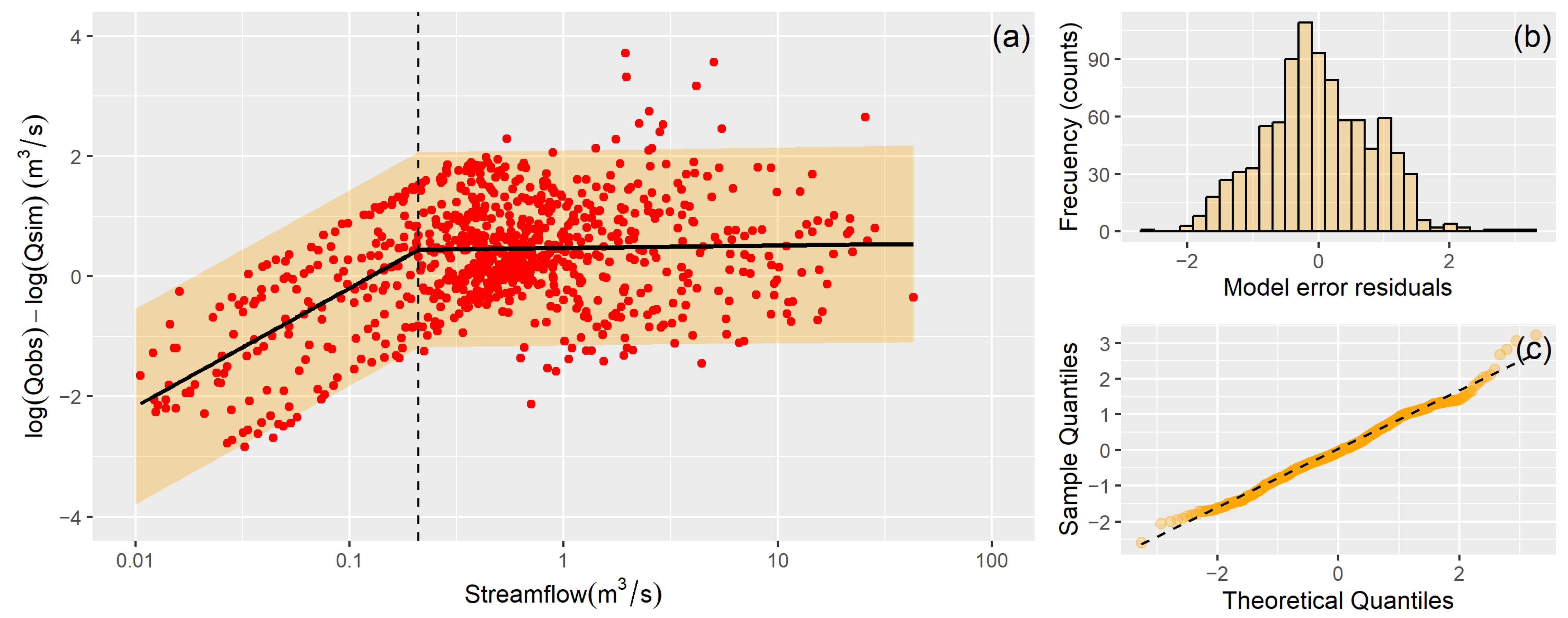
2.3. Goodness-of-Fit Metrics and Error Model for Surface Water

Model performance was evaluated using several goodness-of-fit (GoF) metrics that capture different aspects of accuracy and bias. The Kling–Gupta Efficiency (KGE) and Nash–Sutcliffe Efficiency (NSE) [58] assess how well the model reproduces the variability and dynamics of the observed data; both metrics are dimensionless. Percent bias (PBIAS) reflects the model’s overall tendency to over- or underestimate values. PBIAS in this study is presented as percentages. The normalized root mean square error (nRMSE) expresses the typical error relative to the mean of observations, enabling direct comparison across different observation points or variables with different units or scales; this metric is dimensionless. Mean error (ME) captures the average signed difference between simulated and observed values, while mean absolute error (MAE) measures the average magnitude of these differences regardless of direction. ME and MAE have the same units as the simulations and observations (e.g., surface waters m³/s, groundwater meters). For groundwater, since there are eight observation wells, the overall GoF was estimated by taking the median of the individual metrics. Equations for the GoF used in this study are presented in the supplementary material.

Error models of simulations (also referred to as error models of predictions) is a conceptual framework that aims to explain the relationship between observations and simulations. Depending on the objective, the error model can be formulated in various ways: as the error of the simulations expressed as a function of the simulations themselves; as the error expressed as a function of the observations; as a direct comparison in which observations are modeled as a function of the simulations; as a time series of simulation errors; or by incorporating other explanatory variables such as input uncertainty, model structure or resolution, spatial effects, or autocorrelation. Each formulation serves a different purpose in characterizing uncertainty and identifying systematic deviations. This type of analysis is widely used in the Bayesian Inference, as it helps to identify and address problems related to heteroscedasticity and autocorrelation of model residuals [59]. These approaches can also be used to identify time-dependent patterns in model uncertainty [60], relationships linked to the magnitude of the observations [61], and drifts in groundwater modeling [62], as well as to adjust model simulations or quantify total prediction uncertainty [63,64].

This study focused on total prediction uncertainty; therefore, a logarithmic transformation of surface water model residuals (LSWres) with respect to simulations [60] was applied for surface water (2).

LSW_res ≈ log(Q_sim) − log(Q_obs)

(2)

where LSW_res is the logarithmic residuals of streamflow, Q_obs the observed streamflow, and Q_sim the simulated streamflow. The logarithmic transformation is used because the residuals include many small values. This transformation helps to stabilize the variance and makes the distribution closer to normal.

The error analysis was conducted at the end of the second-phase optimization. The entire simulation period (2018–2021) was considered. No distinction was made between calibration and validation periods, as the objective was to obtain a general behavior of model uncertainties.

The magnitude and nature of model uncertainty can vary depending on the dominant hydrological process, particularly in relation to the simulated streamflow [61]. This is especially relevant during transitions between high-flow periods, driven by direct runoff (rainfall–runoff processes), and low-flow periods, sustained by groundwater contributions (baseflow). To account for potentially distinct sources of uncertainty, a segmented relationship was applied to LSW_res. This allowed the identification of contrasting error structures during high-flow and low-flow conditions.

2.4. Water Pumping and Irrigation Expansion Criteria

It is a challenging task to determine the amount of water extracted from groundwater in Uruguay, as the locations of all pumping wells are not well known, and the volume of water drawn from the aquifer by each well remains unknown. To address this issue, land use involving irrigated crops was identified through a field campaign and by referencing declared irrigation wells in the national database. Pumping wells used for other purposes, such as domestic and livestock water supply, were not considered, as the volume of water used for these purposes is assumed to be negligible compared to irrigation water in the catchment. Once the irrigated crops were identified, it was important to determine the amount of water extracted for irrigation. This volume was estimated based on crop water requirements. However, in practice, irrigation is applied in excess or deficit. For this reason, the water stress threshold that triggers irrigation in the model was calibrated (Table 2). Water stress threshold in SWAT+ ranges from 0 (severe stress, no irrigation) to 1 (no stress, all water requirements are fully satisfied). Setting thresholds between 0.5 and 1 allows the model to simulate irrigation when water stress becomes critical (at 0.5) up to conditions where irrigation is triggered immediately when any water deficit occurs (close to 1). At this stage, citrus, greenhouse horticulture, and open-field horticulture were aggregated with different water stress thresholds. This approach represents the average condition for farmers and allows for differentiation by crop types without the over-parameterization that would result from setting individual thresholds.

The effect of irrigation expansion on baseflow was estimated using the calibrated SWAT+gwflow model over a 25-year period (1999–2023). To this end, it was assumed that irrigation expansion would occur only in areas currently dedicated to rainfed citriculture. This assumption was made on the basis that citriculture plays a crucial role in the local economy, providing employment and contributing to national exports, underscoring its potential for supplementary irrigation. As shown in Figure 1a,b, irrigation expansion could take place in the northern part of the catchment, increasing the total irrigated area from 6193 to 8561 hectares, representing a rise from 30% to 41% of the catchment area. In addition, climate variability was classified based on moisture conditions to analyze water use dynamics in greater detail. Wet moisture conditions were defined as the months in which precipitation exceeded the 66th percentile of the annual monthly precipitation distribution, while dry moisture conditions were those with precipitation below the 33rd percentile. Normal moisture conditions fell between these thresholds (33rd–66th percentiles). This classification provides a clearer understanding of how water use varies according to the combination of rainfall and groundwater irrigation needed to meet crop water requirements.

3. Results

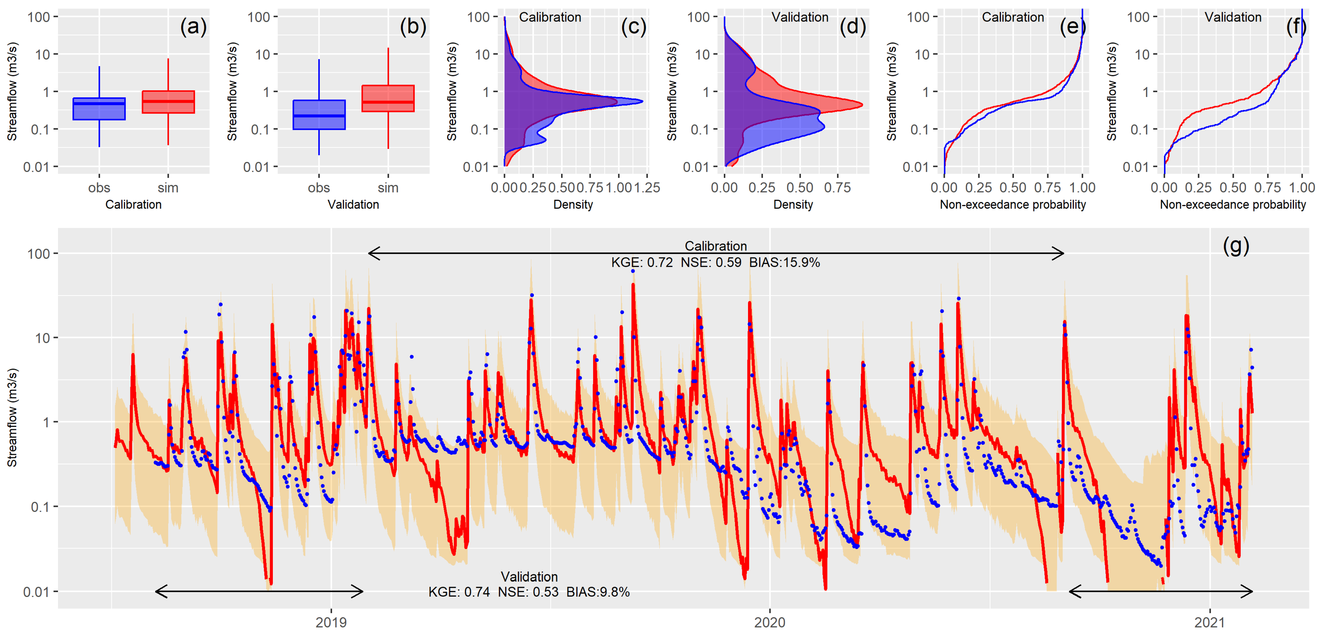
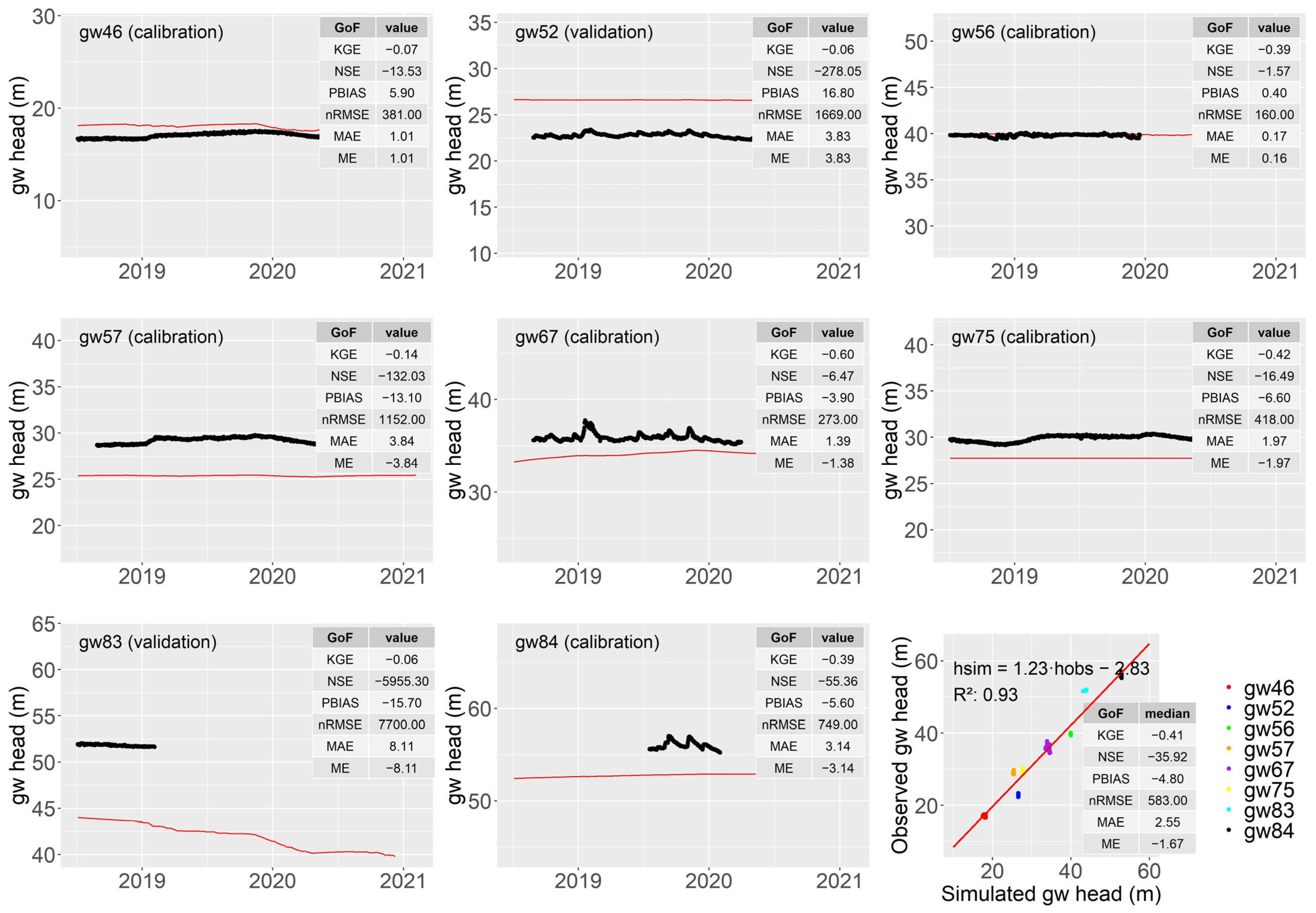
3.1. Model Development

The goodness-of-fit (GoF) metrics are presented in

Table 3. Goodness-of-fit (GoF) metrics for total streamflow (Qt), baseflow (Qb), and the median of the GoF for groundwater heads (GW).

Phase	GoF	Phase I			Phase II
		Qt	Qb	GW	Qt	Qb	GW
Calibration	KGE	0.69	0.43	−0.26	0.72	0.46	−0.41
	NSE	0.56	−0.34	−15.7	0.59	−0.04	−15.0
	PBIAS	14.9	−15.5	−6.9	15.9	16.3	−4.8
	nRMSE	65.9	115	407	63.9	103	399
	MAE	0.97	0.22	1.48	0.86	0.19	1.68
	ME	0.18	−0.06	−2.96	0.19	0.05	−1.67
Validation	KGE	0.68	0.60	−2.27	0.74	0.56	−0.33
	NSE	0.49	0.50	−4331	0.53	0.63	−3116
	PBIAS	15.7	23.9	−9.7	9.8	37.0	0.6
	nRMSE	65.9	115	4733	63.9	103.5	4684
	MAE	1.12	0.18	5.05	0.99	0.14	5.97
	ME	0.23	0.07	−4.95	0.14	0.11	−2.14
Overall	KGE	0.69	0.66	−0.24	0.73	0.67	−0.41
	NSE	0.54	0.29	−52.23	0.57	0.35	−35.92
	PBIAS	15.3	−5.2	−6.9	13.3	20.8	−4.8
	nRMSE	67.7	84.4	679	65.4	80.7	583
	MAE	1.03	0.20	2.96	0.91	0.16	2.55
	ME	0.20	−0.03	−2.96	0.17	0.06	−1.67

for both the calibration and validation periods, along with overall values for the entire simulation period (2018–2021). Phase I yielded reasonable performance (KGE = 0.69, NSE = 0.56) for streamflow, but poor results for groundwater. Phase II shows slight improvements in streamflow and baseflow, along with reduced bias and errors in hydraulic heads (e.g., ME improved from −2.96 to −1.67), though KGE and NSE remain low.

Figure 2 presents the calibration and validation results for the streamflow simulation (Phase II). The box-and-whisker plot (Figure 2a), density function (Figure 2c), and flow duration curve (Figure 2e) demonstrate that the simulated values closely align with the observed data. The streamflow hydrograph shown in Figure 2g is displayed on a logarithmic scale to better highlight and identify the baseflow pattern. Overall, total streamflow is well represented, though the model occasionally underestimates baseflow, with less frequent instances of overestimation (Figure 2g). There are also intervals where baseflow is accurately simulated (e.g., mid-2019). The same types of plots were used for validation (Figure 2b,d,f) to allow for an easy comparison with calibration (Figure 2a,c,e). While a slight decline in performance is visually noticeable during the validation period, the model continues to produce acceptable results, with KGE values of 0.72 for calibration and 0.74 for validation, NSE values of 0.59 for calibration and 0.53 for validation, and BIAS values of 15.9 for calibration and 9.8 for validation. No seasonal biases were detected.

Logarithmic transformation of surface water model residuals (LSW_res) follows a piecewise relationship (Figure 3a). When simulated streamflow is greater than 0.2, LSW_res are normally distributed with a mean of 0.47 and a standard deviation of 0.82. For simulated streamflow values less than 0.2, LSW_res follow a power-law relationship (LSW_res = 5.93Q_sim^0.85, see supplementary material for details on the segmented regression). The error of the piecewise regression follows a normal distribution with zero mean and a standard deviation of 0.83 (Figure 3b,c). This error model was used to determine the 95% total prediction uncertainty shown in Figure 2g.

Figure 4 presents the hydrographs of groundwater levels at the observation wells. Inset tables compare statistics of observations and simulations. In general, the simulated groundwater levels exhibit less variability compared to the observed levels. Among the sites, the greatest variability is observed at the observation well gw67 (Figure 1c), which suggests that this well is more strongly connected to the stream, indicating a rapid response to streamflow changes. In general, the model exhibits poor performance when reproducing groundwater head at the local scale. Additionally, the scatter plot shows a strong correlation between the simulated and observed data, suggesting that errors are, to some extent, compensated across multiple locations.

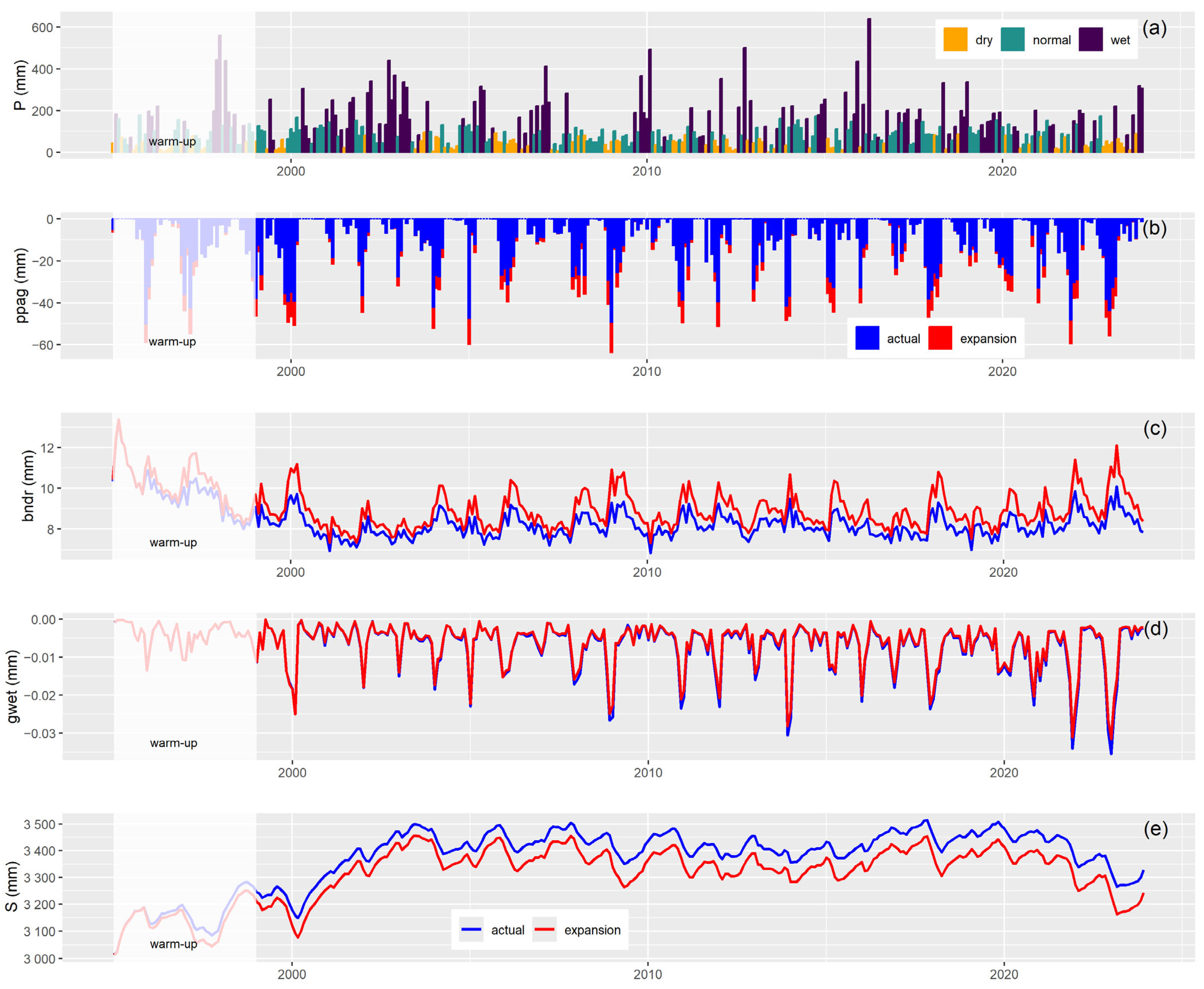
3.2. Irrigation Expansion and Aquifer Water Balance

A 25-year period (1999–2023) was simulated to assess long-term water balances under both current conditions and irrigation expansion.

Table 4. Groundwater balance over a 25-year period under actual conditions and irrigation expansion.

	Inflows (mm)			Outflows (mm)						∆S (mm)
	rech	swgw	bndr	gwet	gwsw	satx	soil	ppag	latl
Actual	316	42,904	2923	−2.32	−1171	−17,869	−23,331	−3446	0	324
Expansion	315	42,712	3148	−2.16	−1165	−17,743	−22,940	−4083	0	241
Difference	−0.32%	−0.45%	7.15%	−7.41%	−0.51%	−0.71%	−1.70%	15.6%	-	−66 *

Note: * Average storage difference expressed as water depth in millimeters with respect to the entire basin area.

presents the overall water balance of the aquifer. The most significant changes in groundwater components are as follows: increased irrigation (15.6%) leads to greater boundary fluxes entering the aquifer (7.15%), along with a minor change in recharge. Evapotranspiration decreases by 7.41%, accompanied by reduced flow from the aquifer into the soil and saturated zone (soil and satx), which may be attributed to a lower water table limiting these fluxes. The net exchange of surface water entering or leaving the aquifer (swgw, gwsw) remains relatively balanced, suggesting that the overall exchange across the catchment is small. ∆S is the storage difference from the beginning of the simulation in 1995 to the end in 2023, and it represents the sum of all inflows and outflows (1). However, these components may have important local impacts, which will be discussed further. The supplementary material shows the daily groundwater balance error to verify that the chosen time step is appropriate.

The irrigation expansion will withdraw 18.4% more water from the aquifer.

Table 5. Average annual pumped water for irrigation for a 25-year period (1999–2023).

	Actual		Expansion
Land Use	Irrigation (mm/yr)	Water Allocation (%)	Irrigation (mm/yr)	Water Allocation (%)
GHCP	3.7	2.7	3.5	2.1
OFCP	22.5	16.3	21.0	12.9
ORAN	111.7	81.0	138.8	85.0
Total	137.9		163.3

presents the volume of irrigation as water depth in millimeters with respect to the entire basin area used by land use and the percentage of water allocation relative to the total water used in the catchment. The sector that consumes the most water is ORAN, followed by OFCP, with only a marginal water allocation for GHCP. This pattern aligns with the land use distribution, which follows a similar trend.

At the catchment scale, monthly precipitation, groundwater storage, and the monthly components of groundwater fluxes that exhibit significant changes are shown in Figure 5. Monthly precipitation (Figure 5a) alternates between dry, normal, and wet periods, with values ranging from near 0 to 640 mm. This wide range highlights the high precipitation variability in the region. Figure 5b illustrates that ppag increases notably during dry months, reflecting greater groundwater use for irrigation. Boundary fluxes are closely related to ppag (Figure 5d); as more water is pumped from the aquifer, the water table lowers, turning the aquifer into a sink, which in turn increases inflow across the catchment boundaries. These partial fluxes, together with other components (rech, swgw, gwsw, satx, soil, and latl, not shown in the figure), drive the changes in monthly groundwater storage (Figure 5e). Storage begins with relatively low initial values, using identical initial conditions for both the actual and irrigation expansion scenarios. After the 4-year warm-up period (1995–1998), the average groundwater storage during the 25-year period (1999–2023) is 3406 mm for the actual scenario and 3340 mm for the irrigation expansion, resulting in a mean difference of −66 mm, with a range from −105 to −31 mm.

The amount of water used largely depends on moisture conditions, with dry periods requiring more supplementary irrigation. Figure 6 shows the monthly water volume used under wet (Figure 6a), normal (Figure 6c), and dry moisture conditions (Figure 6e). During wet moisture conditions, water demand is similar between the actual scenario and the irrigation expansion. Under normal moisture conditions, an increase in water demand is observed from January to April. In dry moisture conditions, water demand is significantly higher, extending from December to April (in this work, regarding boxplots, a significant difference refers to a clear change in the order of magnitude of the mean values and the width of the boxes). This variable water demand, driven by precipitation, also has a fluctuating effect on baseflow. Figure 6f shows that baseflow decreases under irrigation expansion for the location shown in Figure 7, with the effect lagging by four months after the irrigation season. However, under wet conditions (Figure 6b), no significant changes were detected, and under normal moisture conditions (Figure 6d), only a slight decrease in baseflow was observed from June to August.

At the local scale (gwflow grid), annual groundwater depletion of up to −1.2 m is predicted (Figure 6b), with depletion zones closely matching areas of irrigation expansion (Figure 1b) and increasing mean annual pumping rates (Figure 6a). This groundwater depletion directly impacts GW-SW, with the predominant trend being a reduction in baseflows (Figure 6c). However, the spatial pattern of GW-SW indicates that baseflow could also increase in certain areas which are prone to greater contributions from the aquifer.

4. Discussion

4.1. Model Performance

The calibration and validation routines indicate that the model had a good performance for simulating streamflow (Figure 2, Table 3). Streamflow performs similarly in terms of KGE and BIAS to the simulations obtained with the distributed HBV model, presented in a previous study in the same area [41]. The HBV model does not explicitly account for groundwater irrigation; thus, similarities in performance could be due to parameter compensation for the unaccounted irrigation [65]. In addition, over a relatively short period, the goodness-of-fit statistic was in the good to satisfactory range [66], indicating that the selected time frame may be sufficient for calibration and validation. This is relevant, as studies in other regions suggest that the optimal length for calibrating the SWAT model is five to seven years [67]. Factors such as climate variability, land use changes, model structure, length of the calibration/validation windows, and the uncertainty of forcing data are key considerations in defining model uncertainties [60,68,69,70]. Despite the limited length of the simulation period, the model successfully captures key hydrological processes. The two-phase calibration procedure focuses step by step on surface water and groundwater (Table 3). This approach enables simplified calibration, reduces computational costs, and minimizes overfitting [71]. The use of logarithmic transformations in the streamflow hydrograph enables a more detailed assessment of model performance in estimating baseflow, particularly in identifying potential stream–aquifer interactions [72]. Additionally, flow duration curves, probability density functions, and box-and-whisker plots provide complementary insights, allowing for a comprehensive evaluation of how well the model matches the observations. These tools address limitations observed in studies that rely solely on time-series plots or aggregated metrics [73].

The streamflow error model indicates an underestimation of low flows and an overestimation of high flows (Figure 3). LSW_res follows a segmented power-law relationship, meaning that the lower the streamflow, the lower the ratio of simulated to observed streamflow. In contrast, LSW_res associated with high flows are normally distributed around a mean of 0.47, indicating that the ratio of simulated to observed streamflow remains approximately constant. These opposing errors tend to compensate for each other in the overall streamflow prediction, contributing to results with relatively small biases over the simulation period. The different behavior of model residuals depending on the magnitude of simulated streamflow suggests that the error pattern is simulation-dependent, potentially influenced by the dominant hydrological processes under different flow conditions. In addition, the error model shows a good fit and could be used to adjust the simulated streamflow accordingly.

The modeling approach produces groundwater head simulations with greater uncertainty than those reported in previous studies of the same area, which used the MODFLOW model in a fully 3D configuration in steady state conditions, yielding a mean error of 0.67 [44]. Although the current approach results in greater uncertainty (mean error of −1.67) compared to MODFLOW, it offers the advantage of simulating additional processes at spatio-temporal resolutions that MODFLOW cannot achieve. Given that SWAT+gwflow operates with a 100 m groundwater grid size and a global groundwater dataset, the accuracy remains reasonable [74,75]. However, model uncertainty is scale-dependent, and comparisons between models should be made with caution, as different modeling approaches use varying spatial resolutions and conceptual schemes [69]. These differences can affect both the representation of processes and the interpretation of model outputs. As with streamflow, some parameter compensation may also occur in the groundwater simulations.

This work represents the smallest-scale application of SWAT+gwflow to date (225 km²) and expands its use to a new geographic context, beyond the locations previously examined in the USA and Europe.

Table 6. Summary of SWAT+gwflow performance in earlier studies.

Study	∆t	Catchment Area (km2)	Grid Size	Goodness-of-Fit Surface Water	Goodness-of-Fit Groundwater
Little River (USA) [31]	d	327	200	8 stations, NSE (−0.37 to 0.51)	8 wells, MAE (0.4 to 3.0)
Dijle (Belgium) [33]	d	893	200	NSE (0.5), PBIAS (−0.9)	not reported
Winnebago, Nanticoke, Arkansas, Cache (USA) [32]	m	1787 to 7940	500	10 stations, NSE (0.72 to 0.91), KGE (0.80 to 0.91), R2 (0.79 to 0.93), PBIAS (−6.9 to 23.1)	128 wells, ME * (−3.6 to 3.2)
Scheldt (France, Netherlands, Germany) [35]	d	510 to 5817	200 and 500	NSE (0.46 to 0.87)	not reported
Iowa (USA) [62]	d	583	100	NSE (0.86)	4 wells, MAE (1.54)
Klein Nete (Belgium) [35]	d	552	200	NSE (0.86 to 0.91), PBIAS (−2.1 to 9.9)	7 wells, MAE (0.13 to 1.57), RMSE (0.16 to 1.75)
Colorado (USA) [76]	m	7516	250	2 stations, NSE (0.6 to 0.76), KGE (0.68 to 0.69), PBIAS (16 to 21), RMSE (21.2 to 31.7)	not reported
Nanticoke River (USA) [77]	m	2173	500	2 stations, NSE (0.72 to 0.79), KGE (0.83 to 0.86), PBIAS (5.4 to 10.8)	26 wells, MAE (1.1)
Mississippi (USA) [36]	m	2121 to 8210	500	2 stations, NSE (0.59 to 0.91), KGE (0.61 to 0.93), PBIAS (5.7 to 24.4)	1155 wells, ME * (−1.99 to 1.5)
Tagus River (Spain) [78]	d	3274	500	3 stations, NSE (0.59 to 0.86), KGE (0.5 to 0.8), PBIAS (0, 17)	not reported
Arkansas (USA) [79]	m	1839 to 64,000	500	24 stations NSE (0.53 to 0.94), PBIAS (−23.7 to 39.9), R2(0.57 to 0.95)	ME (−2.0 to 2.1)
Arkansas (USA) [80]	m	1874 to 5970	500	7 stations NSE (0.24 to 0.97)	76 wells ME * (−2.0 to 2.1)
Winnebago (USA) [81]	m	1787 to 2141	500	2 stations, NSE (0.74 to 0.93), KGE (0.68 to 0.91), PBIAS (−0.6 to 11.7)	7 + 26 wells, ME (−3.0 to 2.1)
San Antonio (Uruguay) Present study	d	225	100	1 station NSE (0.59), KGE (0.72), PBIAS (15.9)	8 wells, MAE (0.17 to 8.11), ME(−8.11 to 3.83)

Notes: * Reported as MAE with negative values; interpreted here as ME, as MAE is non-negative by definition. m: monthly time step. d: daily time step.

summarizes GoF metrics from earlier studies conducted in catchments ranging from 327 to 64,000 km², providing a basis for comparison with our results. NSE remains a commonly used metric to assess streamflow performance despite its known limitations, such as oversensitivity to high flows and low sensitivity to systematic bias [53]. Reported NSE values range from −0.37 to 0.97, with monthly simulations generally showing better performance. It was more difficult to compare groundwater performance. This is because there are different ways to evaluate model accuracy. The choice depends on the goals of the study and the available observation wells. In some cases, there were no observations, so groundwater simulations could not be verified. In others, there were a few or even many wells, with either continuous or sporadic measurements. In general, NSE and KGE have not been applied to groundwater because these metrics were developed to handle the greater variability and temporal dynamics of surface water time series. Instead, authors often prefer to express model uncertainty using MAE or ME, with RMSE (root mean squared error) used only occasionally. In some cases, depending on data availability and the number of observation wells, studies perform aggregated statistics to summarize performance across stations, which can mask local bias. The diversity of GoF metrics used across studies makes it difficult to compare model performance and limits the ability to identify key sources of uncertainty using standardized criteria. While this variety allows researchers to choose metrics that best fit their data and objectives, it also limits broader perspectives and makes it harder to draw general conclusions across different studies.

4.2. Assessing Irrigation Expansion

The model results indicate groundwater depletion, particularly in regions experiencing irrigation expansion and increasing groundwater extraction (Figure 7b). These findings align with previous studies documented in other regions where groundwater declines in heavily irrigated agricultural areas [11,82]. The observed reductions in baseflows due to irrigation expansion further support established hydrological principles linking groundwater depletion to surface water reductions, where depletion can occur in two ways: an increased flux from streams to the aquifer and a reduced flux from the aquifer to streams. Numerous studies have emphasized that persistent groundwater withdrawals lead to diminished baseflows, reducing streamflow availability during dry periods [83,84]. However, the model also identifies regions where baseflows exhibit an increasing trend (Figure 7c). This result suggests localized groundwater contributions influenced by irrigation return flows [85,86] or higher boundary inflow rates due to inconsistent model boundaries [87].

In regions with highly variable climates, such as Uruguay [43], seasonal fluctuations in precipitation significantly influence irrigation practices, since the water requirements are filled with a combination of infiltrated water from precipitation and groundwater extractions for irrigation [18]. This characteristic leads to variability in pumping rates (Figure 6a,c,e), resulting in differential impacts on baseflows that may affect both water quantity and quality on a seasonal basis [88]. In wet years, when precipitation is abundant, aquifers experience natural recharge, leading to an overall increase in groundwater storage (Figure 5). As a result, the reliance on irrigation water decreases, which in turn reduces the stress on both groundwater reserves and surface water systems. This dynamic also minimizes potential negative impacts on baseflow, as less groundwater extraction translates to more stable streamflow. This characteristic is not considered in current Uruguayan regulations, which assume a constant monthly water supply for irrigation [89]. Conversely, during dry years, aquifers serve as a crucial water source for irrigation, often leading to localized depletion. The extent of this depletion depends on both the intensity of irrigation demands and the precipitation deficit, with the expanding use of groundwater pumping being the primary driver of groundwater depletion worldwide [90]. In some areas, prolonged dry periods can cause significant drawdowns in groundwater levels, potentially leading to hydrological shifts in nearby water bodies.

The lag between groundwater irrigation and its impact on baseflows (Figure 6e,f) arises from the fundamental differences in hydrological processes, velocities, and response times to external forcings such as precipitation variability and/or irrigation timings. Surface water typically responds within hours to days to such inputs, particularly in catchments dependent on surface water irrigation [85]. In contrast, groundwater moves through subsurface pathways at significantly lower velocities (ranging from centimeters to meters per day, depending on the aquifer properties), leading to a delayed response [91]. The impact of groundwater withdrawals on surface water can manifest over timescales from weeks to decades, depending on aquifer properties such as transmissivity, storage capacity, and connection to the stream network [92]. As a result, short-term increases in groundwater pumping may not immediately reduce streamflow, but prolonged pumping can lead to persistent baseflow declines, altering watershed hydrology [93]. A particularly concerning effect is the transition of some stream from perennial to ephemeral flow regimes due to an increase pressure on water resources [94], which can have significant ecological and hydrological consequences [95].

4.3. Model Limitations

Modeling GW-SW dynamics presents several challenges. First, the complex structure of fractured aquifers within the catchment often requires 3D modeling approaches to capture intricate flow patterns [96]. This was simplified with a 2D approach. Second, a major challenge arises from the limited knowledge of water extractions from the aquifer. This challenge was addressed through model calibration, validation, and error estimation, which help to evaluate and adjust for these unknowns. Some authors have tackled this issue in larger catchments using satellite data to better estimate irrigation applications and/or soft-calibration techniques [97,98]. The main advantage of satellite data is that large areas can be easily estimated, avoiding the extensive time required for field surveys. However, these solutions are based upon further estimations that introduce uncertainty. Third, interactions with surrounding areas further complicate the modeling process. At this stage, transient boundary conditions governing how water enters, moves through, and exits the groundwater flow domain can introduce uncertainty [99,100]. Fourth, plains-dominated landscapes can result in low hydraulic gradients, influencing groundwater movement in unexpected ways. Fifth, the small size of the catchment and the reliability of global datasets at such scales may require additional work to achieve the best fit with local datasets [101]. This could be particularly relevant for the aquifer thickness parameter, as partial audiomagnetotelluric scans have revealed that the bedrock of the aquifer follows a pattern, with the aquifer being thinner in the east than in the west of the catchment [42]. Sixth, the relatively short period for model calibration and validation. Usually, long periods are preferred because they may include a wide range of weather conditions, such as droughts or floods. The occurrence of severe droughts could lead to increased pressure on groundwater resources, which could impact the identification of model parameters [102,103], especially aquifer properties, and the quantification of irrigation. Thus, the model should be used with caution in climate change analyses or long memory studies [104,105]. Seventh is the scenario uncertainty itself. The assumed irrigation expansion is expected to occur in the future, but the potential adoption of new irrigation technologies that improve efficiency and reduce water use was neglected. This omission could impact groundwater extractions and return flows. Additionally, climate change was not considered [106], primarily due to the strong assumption that climate variability is the main driver of irrigation scheduling, having a more significant effect on groundwater depletion and baseflow changes than climate change itself. This is particularly relevant in regions with highly variable climates, where identifying the contribution of each component driving these changes remains both a challenge and an opportunity for future research [60].

4.4. Model Benefits

The model is a practical tool for simulating GW-SW in the San Antonio catchment with a relatively low computation cost. This study shows that, although the modeling approach yields a less accurate fit compared to previous studies [44], it still achieves acceptable performance while providing additional benefits in terms of model flexibility and applicability. A key advantage of the model is its ability to incorporate a wide range of hydrological and management scenarios, making it particularly valuable for assessing climate variability and human-induced changes in water resources. Unlike traditional groundwater models, SWAT+gwflow seamlessly integrates surface water and groundwater dynamics while allowing for the inclusion of irrigation pumping schedules and nutrient transport processes in both surface and subsurface flows [31]. Furthermore, the model supports the evaluation of best management practices (BMPs) for environmental impact assessment, such as buffer zones, changes in land use, and optimized irrigation strategies. By linking hydrological and economic analyses, the model facilitates a joint assessment of irrigation expansion and its environmental and economic impacts [107]. This holistic approach enables stakeholders to evaluate trade-offs between agricultural productivity, water resource sustainability, and economic returns, aiding in the development of policies that promote sustainable water use. An additional benefit lies in the use of global datasets and open-source software [45], whose transparent generation processes offer a substantial advantage for ensuring scientific reproducibility, fostering open and inclusive research practices, and enabling future applications and enhancements.

5. Conclusions

This study examined the impact of irrigation expansion on baseflow and groundwater levels, with particular attention to seasonal dynamics. Results confirm that the aquifer and the stream are hydraulically connected, although the strength of this connection varies across different zones of the watershed. Increased groundwater extraction in the summer months led to a delayed effect, reducing baseflow in winter.

These developments have important implications for national water regulations in a country with a highly variable climate, such as Uruguay. It provides valuable information such as spatiotemporal dynamics and the hydraulic connectivity between the aquifer and the stream. Projections carry inherent uncertainties, including assumptions about irrigation practices and aquifer properties. Despite the limitations, the results underscore the need for integrated modeling approaches in regulatory frameworks. Current regulations overlook these interactions due to the lack of integrated modeling approaches and fail to account for seasonal variability in irrigation water demand. Recognizing these dynamics is essential for developing more adaptative and science-based water allocation policies. Doing so would promote irrigation practices, optimize water use without depleting aquifers, and remove key barriers for sustainable agriculture intensification.

References

1. World Meteorological Organization. Unesco International Glossary of Hydrology = Glossaire International d’hydrologie = Mezhdunarodnyĭ Gidrologicheskiĭ Slovarʹ = Glosario Hidrológico Internacional; Secretariat of the World Meteorological Organization: Geneva, Switzerland, 2013; ISBN 978-92-3-001154-3. [Google Scholar]
2. Ketchum, D.; Hoylman, Z.H.; Huntington, J.; Brinkerhoff, D.; Jencso, K.G. Irrigation Intensification Impacts Sustainability of Streamflow in the Western United States. Commun. Earth Environ. 2023, 4, 1–8. [Google Scholar] [CrossRef]
3. Giordano, M.; Mark, F.; Namara, R.; Bassini, E. World Bank Group. 2023. Available online: https://knowledge4policy.ec.europa.eu/publication/impacts-irrigation-review-published-evidence_en (accessed on 13 March 2025).
4. Jasechko, S.; Seybold, H.; Perrone, D.; Fan, Y.; Shamsudduha, M.; Taylor, R.G.; Fallatah, O.; Kirchner, J.W. Rapid Groundwater Decline and Some Cases of Recovery in Aquifers Globally. Nature 2024, 625, 715–721. [Google Scholar] [CrossRef] [PubMed]
5. Haile, G.G.; Tang, Q.; Reda, K.W.; Baniya, B.; He, L.; Wang, Y.; Gebrechorkos, S.H. Projected Impacts of Climate Change on Global Irrigation Water Withdrawals. Agric. Water Manag. 2024, 305, 109144. [Google Scholar] [CrossRef]
6. Pérez-Blanco, C.D.; Hrast-Essenfelder, A.; Perry, C. Irrigation Technology and Water Conservation: A Review of the Theory and Evidence. Rev. Environ. Econ. Policy 2020, 14, 216–239. [Google Scholar] [CrossRef]
7. Bekele, R.D.; Mekonnen, D.; Ringler, C.; Jeuland, M. Irrigation Technologies and Management and Their Environmental Consequences: Empirical Evidence from Ethiopia. Agric. Water Manag. 2024, 302, 109003. [Google Scholar] [CrossRef]
8. Pfeiffer, L.; Lin, C.-Y.C. Does Efficient Irrigation Technology Lead to Reduced Groundwater Extraction? Empirical Evidence. J. Environ. Econ. Manag. 2014, 67, 189–208. [Google Scholar] [CrossRef]
9. Morrisett, C.N.; Van Kirk, R.W.; Bernier, L.O.; Holt, A.L.; Perel, C.B.; Null, S.E. The Irrigation Efficiency Trap: Rational Farm-Scale Decisions Can Lead to Poor Hydrologic Outcomes at the Basin Scale. Front. Environ. Sci. 2023, 11, 1188139. [Google Scholar] [CrossRef]
10. Habets, F.; Philippe, E.; Martin, E.; David, C.H.; Leseur, F. Small Farm Dams: Impact on River Flows and Sustainability in a Context of Climate Change. Hydrol. Earth Syst. Sci. 2014, 18, 4207–4222. [Google Scholar] [CrossRef]
11. Scanlon, B.R.; Faunt, C.C.; Longuevergne, L.; Reedy, R.C.; Alley, W.M.; McGuire, V.L.; McMahon, P.B. Groundwater Depletion and Sustainability of Irrigation in the US High Plains and Central Valley. Proc. Natl. Acad. Sci. USA 2012, 109, 9320–9325. [Google Scholar] [CrossRef]
12. Aderemi, B.A.; Olwal, T.O.; Ndambuki, J.M.; Rwanga, S.S. A Review of Groundwater Management Models with a Focus on IoT-Based Systems. Sustainability 2022, 14, 148. [Google Scholar] [CrossRef]
13. Ray, D.K.; Gerber, J.S.; MacDonald, G.K.; West, P.C. Climate Variation Explains a Third of Global Crop Yield Variability. Nat. Commun. 2015, 6, 5989. [Google Scholar] [CrossRef] [PubMed]
14. Knapp, T.; Huang, Q. Do Climate Factors Matter for Producers’ Irrigation Practices Decisions? J. Hydrol. 2017, 552, 81–91. [Google Scholar] [CrossRef]
15. Xue, J.; Huo, Z.; Kisekka, I. Assessing Impacts of Climate Variability and Changing Cropping Patterns on Regional Evapotranspiration, Yield and Water Productivity in California’s San Joaquin Watershed. Agric. Water Manag. 2021, 250, 106852. [Google Scholar] [CrossRef]
16. Flores Cayuela, C.M.; González Perea, R.; Camacho Poyato, E.; Montesinos, P. An ICT-Based Decision Support System for Precision Irrigation Management in Outdoor Orange and Greenhouse Tomato Crops. Agric. Water Manag. 2022, 269, 107686. [Google Scholar] [CrossRef]
17. Saggi, M.K.; Jain, S. A Survey Towards Decision Support System on Smart Irrigation Scheduling Using Machine Learning Approaches. Arch. Comput. Methods Eng. 2022, 29, 4455–4478. [Google Scholar] [CrossRef]
18. Nie, W.; Zaitchik, B.F.; Rodell, M.; Kumar, S.V.; Arsenault, K.R.; Badr, H.S. Irrigation Water Demand Sensitivity to Climate Variability Across the Contiguous United States. Water Resour. Res. 2021, 57, 2020WR027738. [Google Scholar] [CrossRef]
19. Bosch, H.J.; Gupta, J.; Verrest, H. A Water Property Right Inventory of 60 Countries. Rev. Eur. Comp. Int. Environ. Law 2021, 30, 263–274. [Google Scholar] [CrossRef]
20. Lapides, D.A.; Maitland, B.M.; Zipper, S.C.; Latzka, A.W.; Pruitt, A.; Greve, R. Advancing Environmental Flows Approaches to Streamflow Depletion Management. J. Hydrol. 2022, 607, 127447. [Google Scholar] [CrossRef]
21. Sun, Y.; Chen, X.; Yang, L. Modeling Groundwater-Fed Irrigation and Its Impact on Streamflow and Groundwater Depth in an Agricultural Area of Huaihe River Basin, China. Water 2021, 13, 2220. [Google Scholar] [CrossRef]
22. Sharma, R.; Kumar, R.; Agrawal, P.R.; Ittishree; Chankit; Gupta, G. Chapter 2—Groundwater Extractions and Climate Change. In Water Conservation in the Era of Global Climate Change; Thokchom, B., Qiu, P., Singh, P., Iyer, P.K., Eds.; Elsevier: Amsterdam, The Netherlands, 2021; pp. 23–45. ISBN 978-0-12-820200-5. [Google Scholar]
23. Ntona, M.M.; Busico, G.; Mastrocicco, M.; Kazakis, N. Modeling Groundwater and Surface Water Interaction: An Overview of Current Status and Future Challenges. Sci. Total Environ. 2022, 846, 157355. [Google Scholar] [CrossRef]
24. Norouzi Khatiri, K.; Nematollahi, B.; Hafeziyeh, S.; Niksokhan, M.H.; Nikoo, M.R.; Al-Rawas, G. Groundwater Management and Allocation Models: A Review. Water 2023, 15, 253. [Google Scholar] [CrossRef]
25. Arnold, J.G.; Srinivasan, R.; Muttiah, R.S.; Williams, J.R. Large Area Hydrologic Modeling and Assessment Part I: Model Development1. JAWRA J. Am. Water Resour. Assoc. 1998, 34, 73–89. [Google Scholar] [CrossRef]
26. Akoko, G.; Le, T.H.; Gomi, T.; Kato, T. A Review of SWAT Model Application in Africa. Water 2021, 13, 1313. [Google Scholar] [CrossRef]
27. Aloui, S.; Mazzoni, A.; Elomri, A.; Aouissi, J.; Boufekane, A.; Zghibi, A. A Review of Soil and Water Assessment Tool (SWAT) Studies of Mediterranean Catchments: Applications, Feasibility, and Future Directions. J. Environ. Manag. 2023, 326, 116799. [Google Scholar] [CrossRef] [PubMed]
28. Janjić, J.; Tadić, L. Fields of Application of SWAT Hydrological Model—A Review. Earth 2023, 4, 331–344. [Google Scholar] [CrossRef]
29. Rocha, A.K.P.; De Souza, L.S.B.; De Assunção Montenegro, A.A.; De Souza, W.M.; Da Silva, T.G.F. Revisiting the Application of the SWAT Model in Arid and Semi-Arid Regions: A Selection from 2009 to 2022. Theor. Appl. Climatol. 2023, 154, 7–27. [Google Scholar] [CrossRef]
30. Tan, M.L.; Gassman, P.W.; Srinivasan, R.; Arnold, J.G.; Yang, X. A Review of SWAT Studies in Southeast Asia: Applications, Challenges and Future Directions. Water 2019, 11, 914. [Google Scholar] [CrossRef]
31. Bailey, R.T.; Bieger, K.; Arnold, J.G.; Bosch, D.D. A New Physically-Based Spatially-Distributed Groundwater Flow Module for SWAT+. Hydrology 2020, 7, 75. [Google Scholar] [CrossRef]
32. Abbas, S.A.; Bailey, R.T.; White, J.T.; Arnold, J.G.; White, M.J.; Čerkasova, N.; Gao, J. A Framework for Parameter Estimation, Sensitivity Analysis, and Uncertainty Analysis for Holistic Hydrologic Modeling Using SWAT+. Hydrol. Earth Syst. Sci. 2024, 28, 21–48. [Google Scholar] [CrossRef]
33. Yimer, E.A.; Bailey, R.T.; Piepers, L.L.; Nossent, J.; Van Griensven, A. Improved Representation of Groundwater–Surface Water Interactions Using SWAT+gwflow and Modifications to the Gwflow Module. Water 2023, 15, 3249. [Google Scholar] [CrossRef]
34. Yimer, E.A.; Riakhi, F.-E.; Bailey, R.T.; Nossent, J.; van Griensven, A. The Impact of Extensive Agricultural Water Drainage on the Hydrology of the Kleine Nete Watershed, Belgium. Sci. Total Environ. 2023, 885, 163903. [Google Scholar] [CrossRef] [PubMed]
35. Yimer, E.A.; Bailey, R.T.; Van Schaeybroeck, B.; Van De Vyver, H.; Villani, L.; Nossent, J.; van Griensven, A. Regional Evaluation of Groundwater-Surface Water Interactions Using a Coupled Geohydrological Model (SWAT+Gwflow). J. Hydrol. Reg. Stud. 2023, 50, 101532. [Google Scholar] [CrossRef]
36. Abbas, S.A.; Bailey, R.T.; White, J.T.; Arnold, J.G.; White, M.J. Estimation of Groundwater Storage Loss Using Surface–Subsurface Hydrologic Modeling in an Irrigated Agricultural Region. Sci. Rep. 2025, 15, 8350. [Google Scholar] [CrossRef]
37. Bieger, K.; Arnold, J.G.; Rathjens, H.; White, M.J.; Bosch, D.D.; Allen, P.M.; Volk, M.; Srinivasan, R. Introduction to SWAT +, A Completely Restructured Version of the Soil and Water Assessment Tool. JAWRA J. Am. Water Resour. Assoc. 2017, 53, 115–130. [Google Scholar] [CrossRef]
38. Kim, N.W.; Chung, I.M.; Won, Y.S.; Arnold, J.G. Development and Application of the Integrated SWAT–MODFLOW Model. J. Hydrol. 2008, 356, 1–16. [Google Scholar] [CrossRef]
39. Gao, F.; Feng, G.; Han, M.; Dash, P.; Jenkins, J.; Liu, C. Assessment of Surface Water Resources in the Big Sunflower River Watershed Using Coupled SWAT–MODFLOW Model. Water 2019, 11, 528. [Google Scholar] [CrossRef]
40. Bailey, R.T.; Wible, T.C.; Arabi, M.; Records, R.M.; Ditty, J. Assessing Regional-Scale Spatio-Temporal Patterns of Groundwater–Surface Water Interactions Using a Coupled SWAT-MODFLOW Model. Hydrol. Process. 2016, 30, 4420–4433. [Google Scholar] [CrossRef]
41. Navas, R.; Erasun, V.; Banega, R.; Sapriza, G.; Saracho, A.; Gamazo, P. SanAntonioApp: Interactive Visualization and Repository of Spatially Distributed Flow Duration Curves of the San Antonio Creek—Uruguay. Agrociencia Urug. 2022, 26, e979. [Google Scholar] [CrossRef]
42. Ramos, J.; Blanco, G.; Carráz-Hernández, O.; Corbo-Camargo, F.; Rodríguez-Miranda, W.; Saracho, A.; Borrero, A.; Bessone, L.; Alvareda, E.; Gamazo, P. Geophysical Study of the Salto–Arapey Aquifer System in Salto, Uruguay. J. S. Am. Earth Sci. 2024, 146, 105071. [Google Scholar] [CrossRef]
43. Hu, X.; Eichner, J.; Gong, D.; Barreiro, M.; Kantz, H. Combined Impact of ENSO and Antarctic Oscillation on Austral Spring Precipitation in Southeastern South America (SESA). Clim. Dyn. 2023, 61, 399–412. [Google Scholar] [CrossRef]
44. Erasun, V.; Campet, H.; Vives, L.; Blanco, G.; Banega, R.; Sapriza, G.; Gaye, M.; Ramos, J.; Alvareda, E.; Gamazo, P.; et al. Modelación Del Sistema Acuífero Salto Arapey (Uruguay). Rev. Lat.-Am. Hidrogeol. 2020, 11, 68–75. [Google Scholar]
45. Navas, R.; Gelos, M. SWAT+gwflow San Antonio Basin—Uruguay. OSF, 16 May 2025. [Google Scholar] [CrossRef]
46. Peel, M.C.; Finlayson, B.L.; McMahon, T.A. Updated World Map of the Köppen-Geiger Climate Classification. Hydrol. Earth Syst. Sci. 2007, 11, 1633–1644. [Google Scholar] [CrossRef]
47. MGAP. Mapa Integrado de Cobertura/uso del Suelo del Uruguay año 2018. Available online: https://www.gub.uy/ministerio-ganaderia-agricultura-pesca/comunicacion/publicaciones/mapa-integrado-coberturauso-del-suelo-del-uruguay-ano-2018 (accessed on 25 January 2025).
48. RENARE. Mapa General de Suelos Del Uruguay, Según Soil Taxonomy USDA. Available online: https://visualizador.ide.uy/geonetwork/srv/api/records/1335f1c8-65eb-46df-8fba-9310a338e692 (accessed on 10 August 2021).
49. Blanco, G.; Abre, P.; Ferrizo, H.; Gaye, M.; Gamazo, P.; Ramos, J.; Alvareda, E.; Saracho, A. Revealing Weathering, Diagenetic and Provenance Evolution Using Petrography and Geochemistry: A Case of Study from the Cretaceous to Cenozoic Sedimentary Record of the SE Chaco-Paraná Basin in Uruguay. J. S. Am. Earth Sci. 2021, 105, 102974. [Google Scholar] [CrossRef]
50. Huscroft, J.; Gleeson, T.; Hartmann, J.; Börker, J. Compiling and Mapping Global Permeability of the Unconsolidated and Consolidated Earth: GLobal HYdrogeology MaPS 2.0 (GLHYMPS 2.0). Geophys. Res. Lett. 2018, 45, 1897–1904. [Google Scholar] [CrossRef]
51. Hengl, T.; Mendes De Jesus, J.; Heuvelink, G.B.M.; Ruiperez Gonzalez, M.; Kilibarda, M.; Blagotić, A.; Shangguan, W.; Wright, M.N.; Geng, X.; Bauer-Marschallinger, B.; et al. SoilGrids250m: Global Gridded Soil Information Based on Machine Learning. PLoS ONE 2017, 12, e0169748. [Google Scholar] [CrossRef] [PubMed]
52. SWAT+ Development Team Gwflow Module for SWAT+. Available online: https://swat.tamu.edu/software/plus/gwflow/ (accessed on 28 April 2025).
53. Gupta, H.V.; Kling, H.; Yilmaz, K.K.; Martinez, G.F. Decomposition of the Mean Squared Error and NSE Performance Criteria: Implications for Improving Hydrological Modelling. J. Hydrol. 2009, 377, 80–91. [Google Scholar] [CrossRef]
54. Althoff, D.; Rodrigues, L.N. Goodness-of-Fit Criteria for Hydrological Models: Model Calibration and Performance Assessment. J. Hydrol. 2021, 600, 126674. [Google Scholar] [CrossRef]
55. SWAT+ Development Team Introduction to SWAT+ | SWAT+ Documentation. Available online: https://swatplus.gitbook.io/io-docs (accessed on 28 April 2025).
56. Kang, T.; Lee, S.; Lee, N.; Jin, Y. Baseflow Separation Using the Digital Filter Method: Review and Sensitivity Analysis. Water 2022, 14, 485. [Google Scholar] [CrossRef]
57. Samsonov, T. Grwat: River Hydrograph Separation and Analysis 2022, Version 0.0.4; Available online: https://CRAN.R-project.org/package=grwat (accessed on 28 April 2025). [CrossRef]
58. Nash, J.E.; Sutcliffe, J.V. River Flow Forecasting through Conceptual Models Part I—A Discussion of Principles. J. Hydrol. 1970, 10, 282–290. [Google Scholar] [CrossRef]
59. Smith, T.; Marshall, L.; Sharma, A. Modeling Residual Hydrologic Errors with Bayesian Inference. J. Hydrol. 2015, 528, 29–37. [Google Scholar] [CrossRef]
60. Navas, R.; Alonso, J.; Gorgoglione, A.; Vervoort, R.W. Identifying Climate and Human Impact Trends in Streamflow: A Case Study in Uruguay. Water 2019, 11, 1433. [Google Scholar] [CrossRef]
61. Navas, R.; Gamazo, P.; Vervoort, R.W. Bayesian Inference of Synthetic Daily Rating Curves by Coupling Chebyshev Polynomials and the GR4J Model. In Proceedings of the IAHS, Montpellier, France, 29 May–3 June 2022; Copernicus GmbH: Göttingen, Germany, 2024; Volume 385, pp. 399–406. [Google Scholar]
62. Bailey, R.T.; Bieger, K.; Flores, L.; Tomer, M. Evaluating the Contribution of Subsurface Drainage to Watershed Water Yield Using SWAT+ with Groundwater Modeling. Sci. Total Environ. 2022, 802, 149962. [Google Scholar] [CrossRef]
63. Han, H.; Morrison, R.R. Improved Runoff Forecasting Performance through Error Predictions Using a Deep-Learning Approach. J. Hydrol. 2022, 608, 127653. [Google Scholar] [CrossRef]
64. Renard, B.; Kavetski, D.; Kuczera, G.; Thyer, M.; Franks, S.W. Understanding Predictive Uncertainty in Hydrologic Modeling: The Challenge of Identifying Input and Structural Errors. Water Resour. Res. 2010, 46, W05521. [Google Scholar] [CrossRef]
65. Lan, T.; Lin, K.; Xu, C.-Y.; Tan, X.; Chen, X. Dynamics of Hydrological-Model Parameters: Mechanisms, Problems and Solutions. Hydrol. Earth Syst. Sci. 2020, 24, 1347–1366. [Google Scholar] [CrossRef]
66. Moriasi, D.N.; Arnold, J.G.; Van Liew, M.W.; Bingner, R.L.; Harmel, R.D.; Veith, T.L. Model Evaluation Guidelines for Systematic Quantification of Accuracy in Watershed Simulations. Trans. ASABE 2007, 50, 885–900. [Google Scholar] [CrossRef]
67. Ziarh, G.F.; Kim, J.H.; Song, J.Y.; Chung, E.-S. Quantifying Uncertainty in Runoff Simulation According to Multiple Evaluation Metrics and Varying Calibration Data Length. Water 2024, 16, 517. [Google Scholar] [CrossRef]
68. Mockler, E.M.; Chun, K.P.; Sapriza-Azuri, G.; Bruen, M.; Wheater, H.S. Assessing the Relative Importance of Parameter and Forcing Uncertainty and Their Interactions in Conceptual Hydrological Model Simulations. Adv. Water Resour. 2016, 97, 299–313. [Google Scholar] [CrossRef]
69. Navas, R.; Delrieu, G. Distributed Hydrological Modeling of Floods in the Cévennes-Vivarais Region, France: Impact of Uncertainties Related to Precipitation Estimation and Model Parameterization. J. Hydrol. 2018, 565, 276–288. [Google Scholar] [CrossRef]
70. Shen, H.; Tolson, B.A.; Mai, J. Time to Update the Split-Sample Approach in Hydrological Model Calibration. Water Resour. Res. 2022, 58, e2021WR031523. [Google Scholar] [CrossRef]
71. Wi, S.; Yang, Y.C.E.; Steinschneider, S.; Khalil, A.; Brown, C.M. Calibration Approaches for Distributed Hydrologic Models Using High Performance Computing: Implication for Streamflow Projections under Climate Change. Hydrol. Earth Syst. Sci. Discuss. 2014, 11, 10273–10317. [Google Scholar]
72. Thomas, B.F.; Vogel, R.M.; Famiglietti, J.S. Objective Hydrograph Baseflow Recession Analysis. J. Hydrol. 2015, 525, 102–112. [Google Scholar] [CrossRef]
73. Westerberg, I.K.; Guerrero, J.-L.; Younger, P.M.; Beven, K.J.; Seibert, J.; Halldin, S.; Freer, J.E.; Xu, C.-Y. Calibration of Hydrological Models Using Flow-Duration Curves. Hydrol. Earth Syst. Sci. 2011, 15, 2205–2227. [Google Scholar] [CrossRef]
74. Vermeulen, P.T.M.; te Stroet, C.B.M.; Heemink, A.W. Limitations to Upscaling of Groundwater Flow Models Dominated by Surface Water Interaction. Water Resour. Res. 2006, 42, W10406. [Google Scholar] [CrossRef]
75. Wan, W.; Döll, P.; Müller Schmied, H. Global-Scale Groundwater Recharge Modeling Is Improved by Tuning Against Ground-Based Estimates for Karst and Non-Karst Areas. Water Resour. Res. 2024, 60, e2023WR036182. [Google Scholar] [CrossRef]
76. Schulz, E.Y.; Morrison, R.R.; Bailey, R.T.; Raffae, M.; Arnold, J.G.; White, M.J. River Corridor Beads Are Important Areas of Floodplain-groundwater Exchange within the Colorado River Headwaters Watershed. Hydrol. Process. 2024, 38, e15282. [Google Scholar] [CrossRef]
77. Tuladhar, A.; Bailey, R.T.; Abbas, S.A.; Shanmugam, M.S.; Arnold, J.G.; White, M.J. Quantifying the Impact of Climate Change and Land Use Change on Surface-Subsurface Nutrient Dynamics in a Chesapeake Bay Watershed System. J. Environ. Manag. 2025, 380, 125101. [Google Scholar] [CrossRef]
78. Castellanos-Osorio, G.; Abbas, S.A.; Molina-Navarro, E.; Bailey, R.T.; Senent-Aparicio, J. Assessing Improvements in Environmental Flow Estimation through the Use of a Coupled Surface-Groundwater Model. Groundw. Sustain. Dev. 2025, 29, 101426. [Google Scholar] [CrossRef]
79. Abbas, S.A.; Bailey, R.T.; Arnold, J.G.; White, M.J.; Mirchi, A. Modeling Agro-Hydrological Surface-Subsurface Processes in a Semi-Arid, Intensively Irrigated River Basin. J. Hydrol. Reg. Stud. 2025, 57, 102188. [Google Scholar] [CrossRef]
80. Bailey, R.T.; Abbas, S.; Arnold, J.G.; White, M.J. Assessing Selenium Fate and Transport in a Semi-Arid River Basin with and without Human Influence. Water Res. 2025, 277, 123335. [Google Scholar] [CrossRef]
81. Abbas, S.A.; Bailey, R.T.; White, J.T.; Arnold, J.G.; White, M.J. Quantifying the Role of Calibration Strategies on Surface-Subsurface Hydrologic Model Performance. Hydrol. Process. 2024, 38, e15298. [Google Scholar] [CrossRef]
82. Kazakis, N.; Karakatsanis, D.; Ntona, M.M.; Polydoropoulos, K.; Zavridou, E.; Voudouri, K.A.; Busico, G.; Kalaitzidou, K.; Patsialis, T.; Perdikaki, M.; et al. Groundwater Depletion. Are Environmentally Friendly Energy Recharge Dams a Solution? Water 2024, 16, 1541. [Google Scholar] [CrossRef]
83. Brutsaert, W. Long-Term Groundwater Storage Trends Estimated from Streamflow Records: Climatic Perspective. Water Resour. Res. 2008, 44, W02409. [Google Scholar] [CrossRef]
84. Sophocleous, M. Interactions between Groundwater and Surface Water: The State of the Science. Hydrogeol. J. 2002, 10, 52–67. [Google Scholar] [CrossRef]
85. Saracho, A.; Navas, R.; Gamazo, P.; Alvareda, E. Assessing Impacts of Irrigation on Flows Frequency Downstream of an Irrigated Agricultural System by the SWAT Model. In Proceedings of the IAHS, Montpellier, France, 29 May–3 June 2022; Copernicus GmbH: Göttingen, Germany, 2024; Volume 385, pp. 423–427. [Google Scholar]
86. Tulip, S.S.; Siddik, M.S.; Islam, M.N.; Rahman, A.; Torabi Haghighi, A.; Mustafa, S.M.T. The Impact of Irrigation Return Flow on Seasonal Groundwater Recharge in Northwestern Bangladesh. Agric. Water Manag. 2022, 266, 107593. [Google Scholar] [CrossRef]
87. Li, W.; Wang, L.; Zhang, Y.; Wu, L.; Zeng, L.; Tuo, Z. Determining the Groundwater Basin and Surface Watershed Boundary of Dalinuoer Lake in the Middle of Inner Mongolian Plateau, China and Its Impacts on the Ecological Environment. China Geol. 2021, 4, 498–508. [Google Scholar] [CrossRef]
88. Pinardi, M.; Soana, E.; Severini, E.; Racchetti, E.; Celico, F.; Bartoli, M. Agricultural Practices Regulate the Seasonality of Groundwater-River Nitrogen Exchanges. Agric. Water Manag. 2022, 273, 107904. [Google Scholar] [CrossRef]
89. DINAGUA Solicitud de Derechos de Uso de Agua | Trámites. Available online: https://www.gub.uy/tramites/solicitud-derechos-uso-agua (accessed on 27 April 2025).
90. Monir, M.M.; Sarker, S.C.; Islam, A.R.M.T. A Critical Review on Groundwater Level Depletion Monitoring Based on GIS and Data-Driven Models: Global Perspectives and Future Challenges. HydroResearch 2024, 7, 285–300. [Google Scholar] [CrossRef]
91. Schreiner-McGraw, A.P.; Ajami, H. Delayed Response of Groundwater to Multi-Year Meteorological Droughts in the Absence of Anthropogenic Management. J. Hydrol. 2021, 603, 126917. [Google Scholar] [CrossRef]
92. Mukherjee, A.; Bhanja, S.N.; Wada, Y. Groundwater Depletion Causing Reduction of Baseflow Triggering Ganges River Summer Drying. Sci. Rep. 2018, 8, 12049. [Google Scholar] [CrossRef]
93. Scanlon, B.R.; Pool, D.R.; Rateb, A.; Conway, B.; Sorensen, K.; Udall, B.; Reedy, R.C. Multidecadal Drought Impacts on the Lower Colorado Basin with Implications for Future Management. Commun. Earth Environ. 2025, 6, 1–13. [Google Scholar] [CrossRef]
94. Gutiérrez-Jurado, K.Y.; Partington, D.; Batelaan, O.; Cook, P.; Shanafield, M. What Triggers Streamflow for Intermittent Rivers and Ephemeral Streams in Low-Gradient Catchments in Mediterranean Climates. Water Resour. Res. 2019, 55, 9926–9946. [Google Scholar] [CrossRef]
95. Nabih, S.; Tzoraki, O.; Zanis, P.; Tsikerdekis, T.; Akritidis, D.; Kontogeorgos, I.; Benaabidate, L. Alteration of the Ecohydrological Status of the Intermittent Flow Rivers and Ephemeral Streams Due to the Climate Change Impact (Case Study: Tsiknias River). Hydrology 2021, 8, 43. [Google Scholar] [CrossRef]
96. Cai, J.; Su, Y.; Shen, H.; Huang, Y. Simulation of Groundwater Flow in Fractured-Karst Aquifer with a Coupled Model in Maling Reservoir, China. Appl. Sci. 2021, 11, 1888. [Google Scholar] [CrossRef]
97. Arnold, J.G.; Youssef, M.A.; Yen, H.; White, M.J.; Sheshukov, A.Y.; Sadeghi, A.M.; Moriasi, D.N.; Steiner, J.L.; Amatya, D.; Skaggs, R.W.; et al. Hydrological Processes and Model Representation: Impact of Soft Data on Calibration. Am. Soc. Agric. Biololgical Eng. 2015, 58, 1637–1660. [Google Scholar] [CrossRef]
98. Brochet, E.; Grusson, Y.; Sauvage, S.; Lhuissier, L.; Demarez, V. How to Account for Irrigation Withdrawals in a Watershed Model. Hydrol. Earth Syst. Sci. 2024, 28, 49–64. [Google Scholar] [CrossRef]
99. Meyer, R.; Greskowiak, J.; Seibert, S.L.; Post, V.E.; Massmann, G. Effects of Boundary Conditions and Aquifer Parameters on Salinity Distribution and Mixing-Controlled Reactions in High-Energy Beach Aquifers. Hydrol. Earth Syst. Sci. 2025, 29, 1469–1482. [Google Scholar] [CrossRef]
100. Gaiolini, M.; Colombani, N.; Busico, G.; Rama, F.; Mastrocicco, M. Impact of Boundary Conditions Dynamics on Groundwater Budget in the Campania Region (Italy). Water 2022, 14, 2462. [Google Scholar] [CrossRef]
101. Condon, L.E.; Kollet, S.; Bierkens, M.F.P.; Fogg, G.E.; Maxwell, R.M.; Hill, M.C.; Fransen, H.H.; Verhoef, A.; Van Loon, A.F.; Sulis, M.; et al. Global Groundwater Modeling and Monitoring: Opportunities and Challenges. Water Resour. Res. 2021, 57, e2020WR029500. [Google Scholar] [CrossRef]
102. Zhao, B.; Mao, J.; Dai, Q.; Han, D.; Dai, H.; Rong, G. Exploration on Hydrological Model Calibration by Considering the Hydro-Meteorological Variability. Hydrol. Res. 2019, 51, 30–46. [Google Scholar] [CrossRef]
103. Yang, W.; Xia, R.; Chen, H.; Wang, M.; Xu, C.-Y. The Impact of Calibration Conditions on the Transferability of Conceptual Hydrological Models under Stationary and Nonstationary Climatic Conditions. J. Hydrol. 2022, 613, 128310. [Google Scholar] [CrossRef]
104. de Lavenne, A.; Andréassian, V.; Crochemore, L.; Lindström, G.; Arheimer, B. Quantifying Multi-Year Hydrological Memory with Catchment Forgetting Curves. Hydrol. Earth Syst. Sci. 2022, 26, 2715–2732. [Google Scholar] [CrossRef]
105. Chaves, H.M.L.; Lorena, D.R. Assessing Reservoir Reliability Using Classical and Long-Memory Statistics. J. Hydrol. Reg. Stud. 2019, 26, 100641. [Google Scholar] [CrossRef]
106. Ahmed, W.; Ahmed, S.; Punthakey, J.F.; Dars, G.H.; Ejaz, M.S.; Qureshi, A.L.; Mitchell, M. Statistical Analysis of Climate Trends and Impacts on Groundwater Sustainability in the Lower Indus Basin. Sustainability 2024, 16, 441. [Google Scholar] [CrossRef]
107. Souto, A.; Carriquiry, M.; Rosas, F. An Integrated Assessment Model of the Impacts of Agricultural Intensification: Trade-offs between Economic Benefits and Water Quality under Uncertainty. Aust. J. Agric. Resour. Econ. 2024, 68, 315–334. [Google Scholar] [CrossRef]
Figure 1. (a) Land use, (b) irrigation scenarios, (c) hypsometry, stations for observation of surface water (sw) and groundwater (gw), (d) steady state hydraulic head, (e) hydraulic conductivity zones, (f) aquifer thickness for the San Antonio catchment—Uruguay.
Water 17 01680 g001
Figure 2. Model performance for streamflow (location: San Antonio at Ruta 3, sw107): (a,b) boxplots, (c,d) probability density function, (e,f) flow duration curves, (g) surface water hydrographs of observations (blue) and simulations (red) for the (a,c,e) calibration, and the (b,d,f) validation periods and 95% of prediction uncertainty (orange).
Water 17 01680 g002
Figure 3. (a) Streamflow logarithmic residuals as a function of simulated streamflow, (b) histogram, and (c) Q-Q plot of errors of the piecewise relationship (location: San Antonio at Ruta 3, sw107).
Water 17 01680 g003
Figure 4. Hydrographs of groundwater levels (simulations: red line, observations: black points) with the goodness-of-fit statistics in the inset table, alongside a scatter plot of observations and simulations.
Water 17 01680 g004
Figure 5. Monthly (a) precipitation, (b) irrigation, (c) boundary fluxes, (d) groundwater evaporation, and (e) storage, expressed as water depth in millimeters with respect to the entire basin area.
Water 17 01680 g005
Figure 6. (a,c,e) Monthly water allocation at the catchment scale and (b,d,f) baseflow response for the San Antonio at Garibaldi (shown in Figure 7), under (a,b) wet, (c,d) normal, and (e,f) dry conditions, for both actual and future irrigation expansion over a 25-year period (1999–2023). Irrigation as water depth in millimeters with respect to the entire basin area.
Water 17 01680 g006
Figure 7. Irrigation expansion effect on (a) mean annual pumping rates, (b) groundwater head, and (c) mean annual groundwater–surface water exchanges (positive values indicate more transfer of water from the stream to the aquifer). The yellow diamond marks the location of the San Antonio at Garibaldi for the analysis presented in Figure 6.
Water 17 01680 g007