


Trophic State Evolution of 45 Yellowstone Lakes over Two Decades: Field Data and a Longitudinal Study


 , , , ,
Abstract

1. Introduction
2. Methods
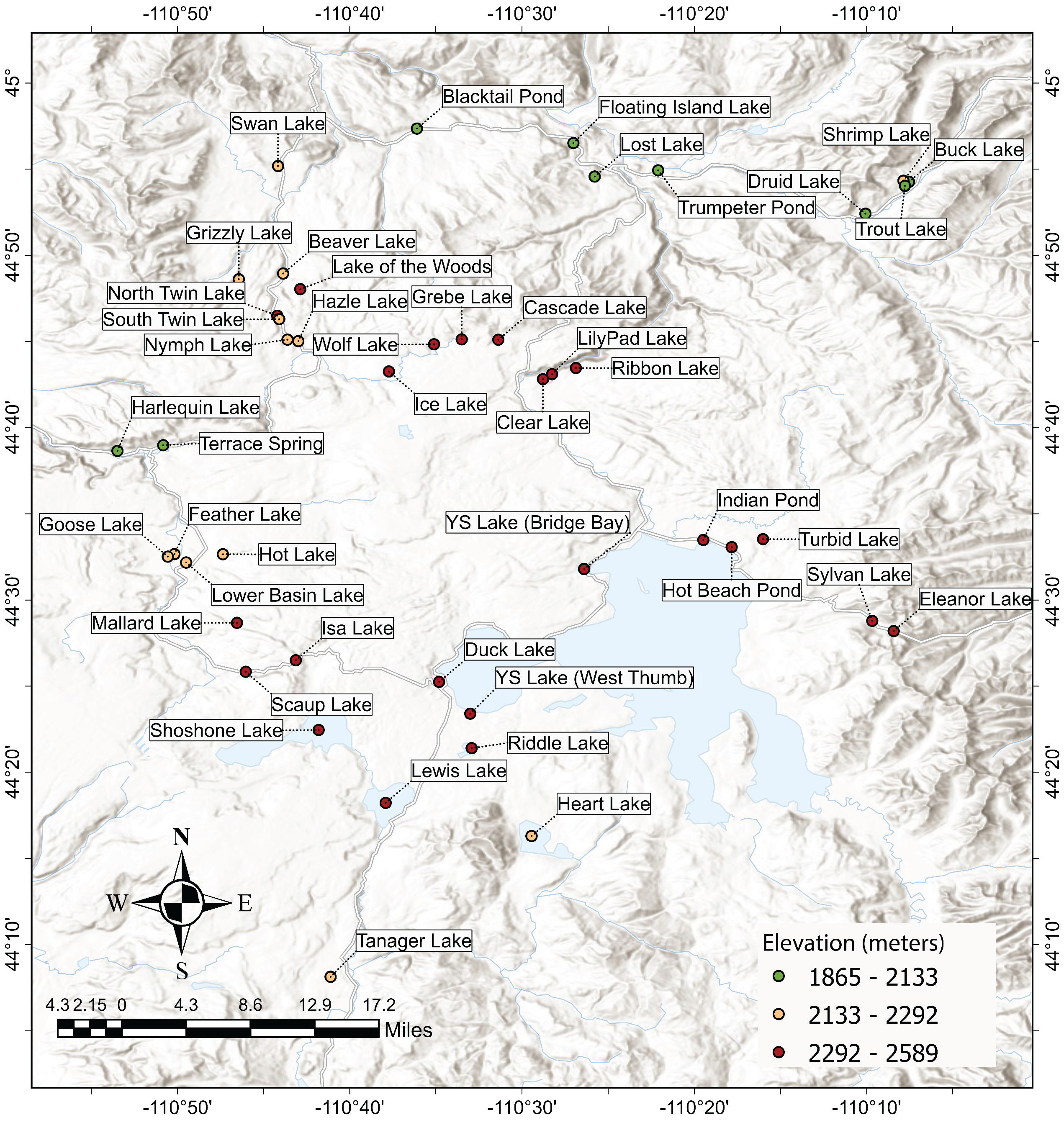
2.1. Study Area
2.2. Data
2.2.1. Field Data Collection
2.2.2. Physical Parameters
2.3. Trophic State Models
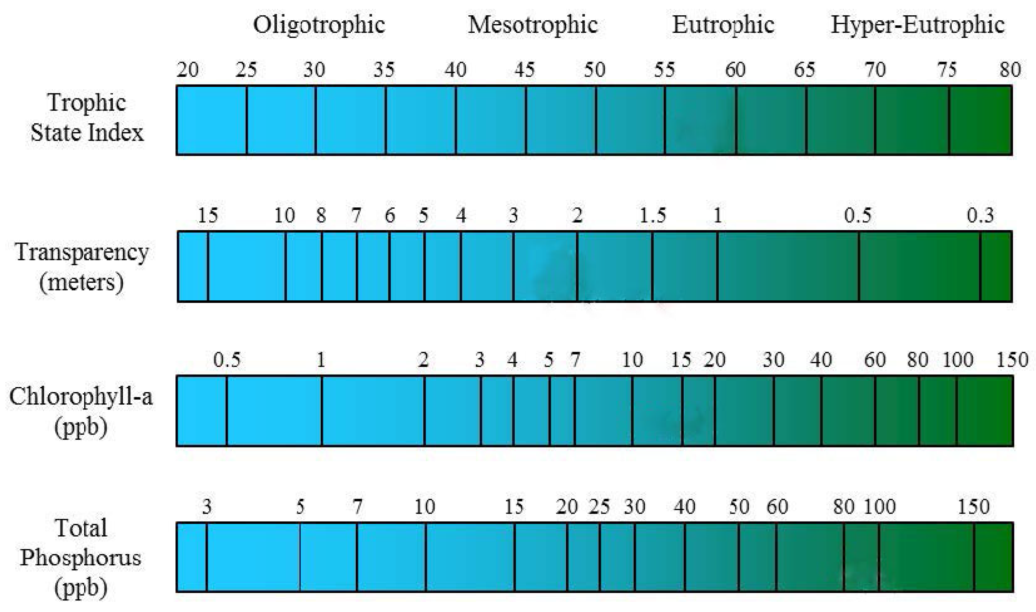
2.3.1. Trophic State Model Overview
2.3.2. CTSI Model
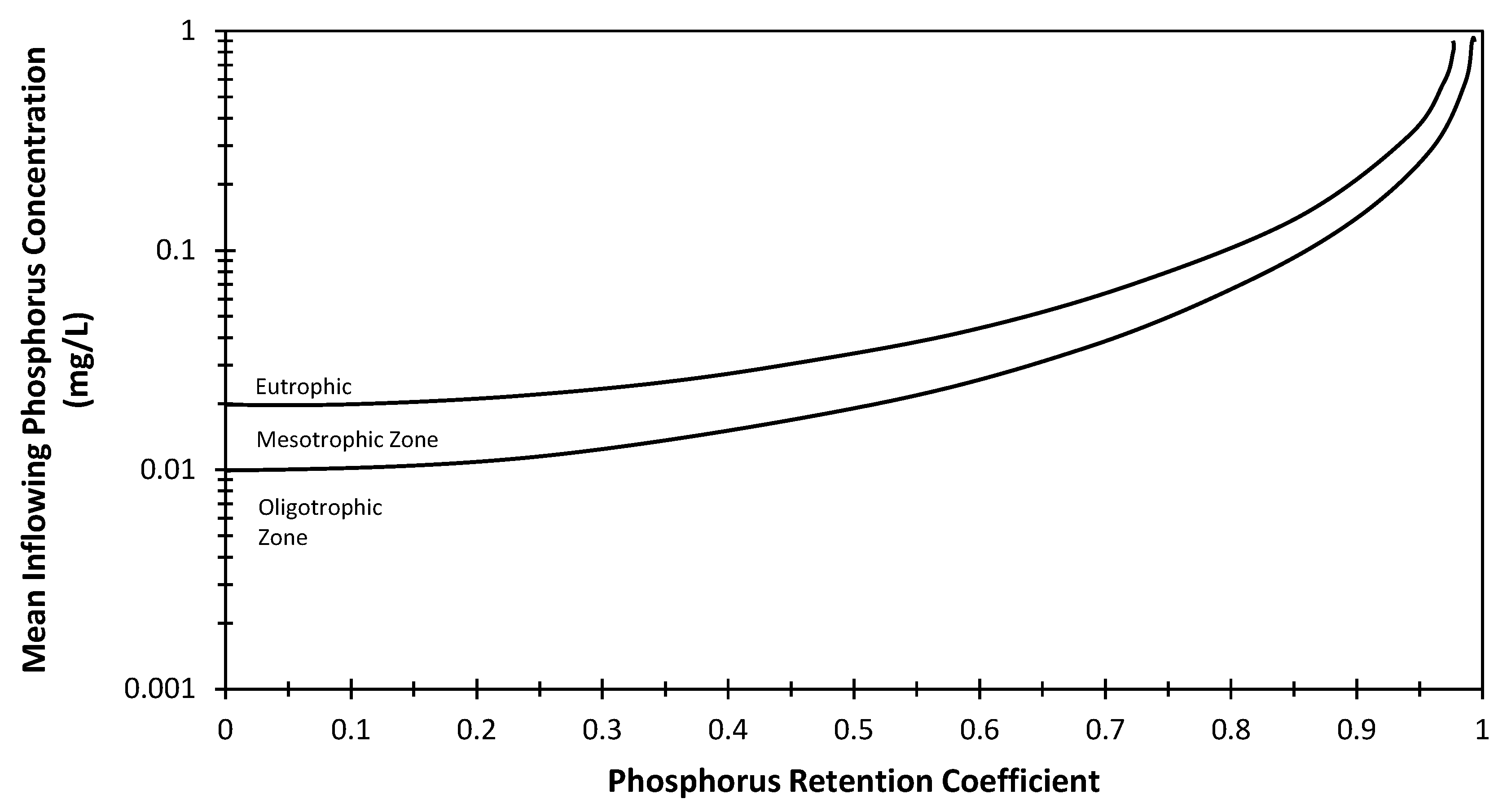
2.3.3. VW Model
2.3.4. LM Model
2.4. Trend Analysis
2.5. Statistical Grouping
- (1)
- Pearson’s correlation coefficient (r):where r ranges from −1 to +1, indicating the strength and direction of linear relationships between variables, and where ±1 represents perfect correlation and 0 indicates no correlation.
- (2)
- Coefficient of determination (R2):where R2 represents the proportion of variance in the dependent variable explained by the independent variable, ranging from 0 to 1, and where 1 indicates perfect prediction.
- (3)
- p-values: which show the probability of obtaining test results at least as extreme as the observed results under the null hypothesis (no relationship between variables). A p-value < 0.05 indicates statistical significance or a 5% chance the result is because of variance in the dataset, rather than an actual difference.
3. Results and Discussion
3.1. Data Analysis
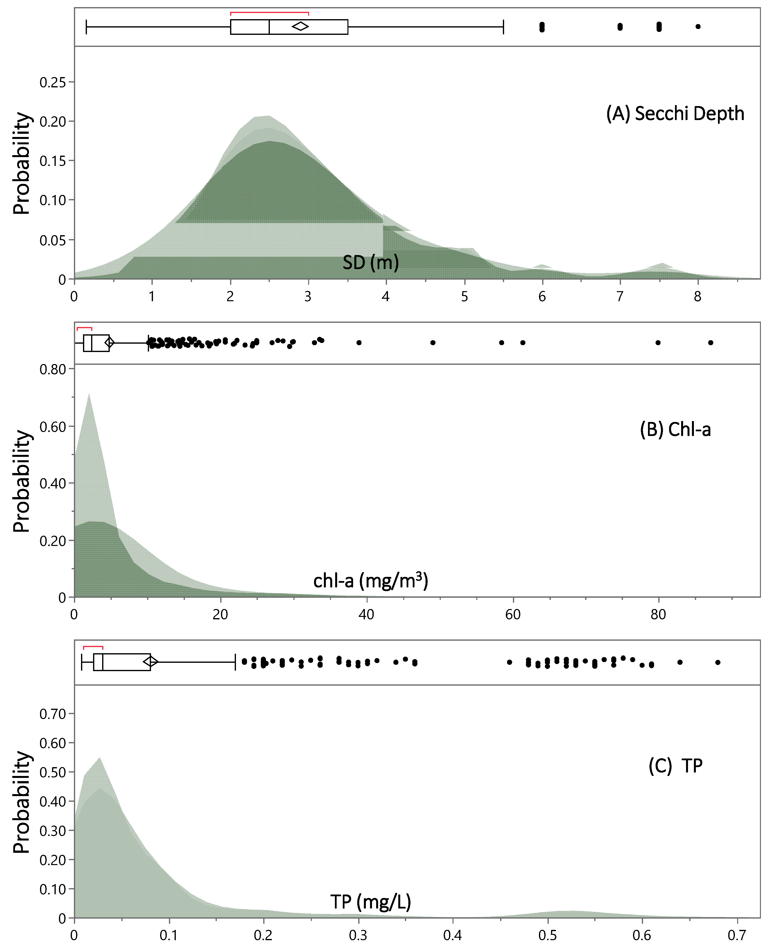
3.1.1. Data Statistical Distributions
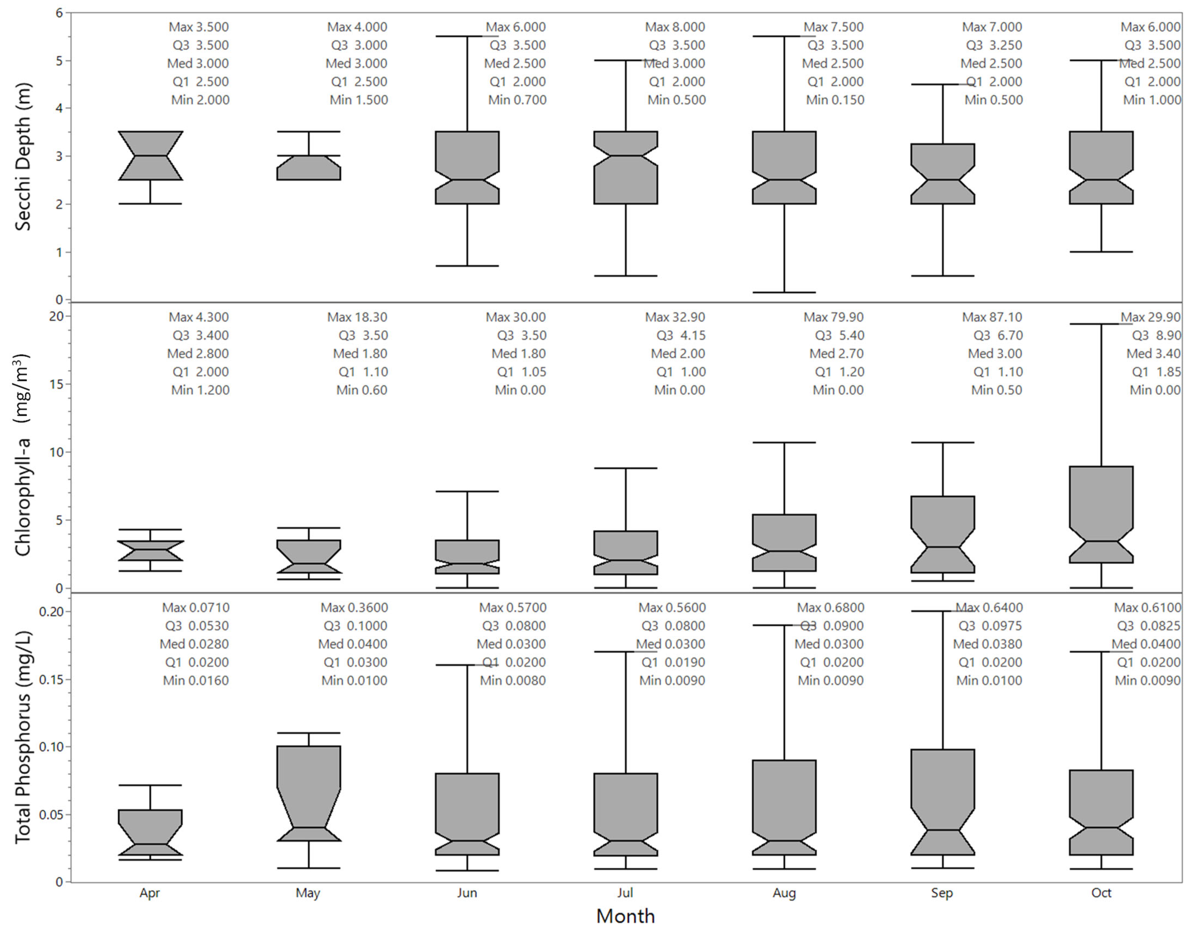
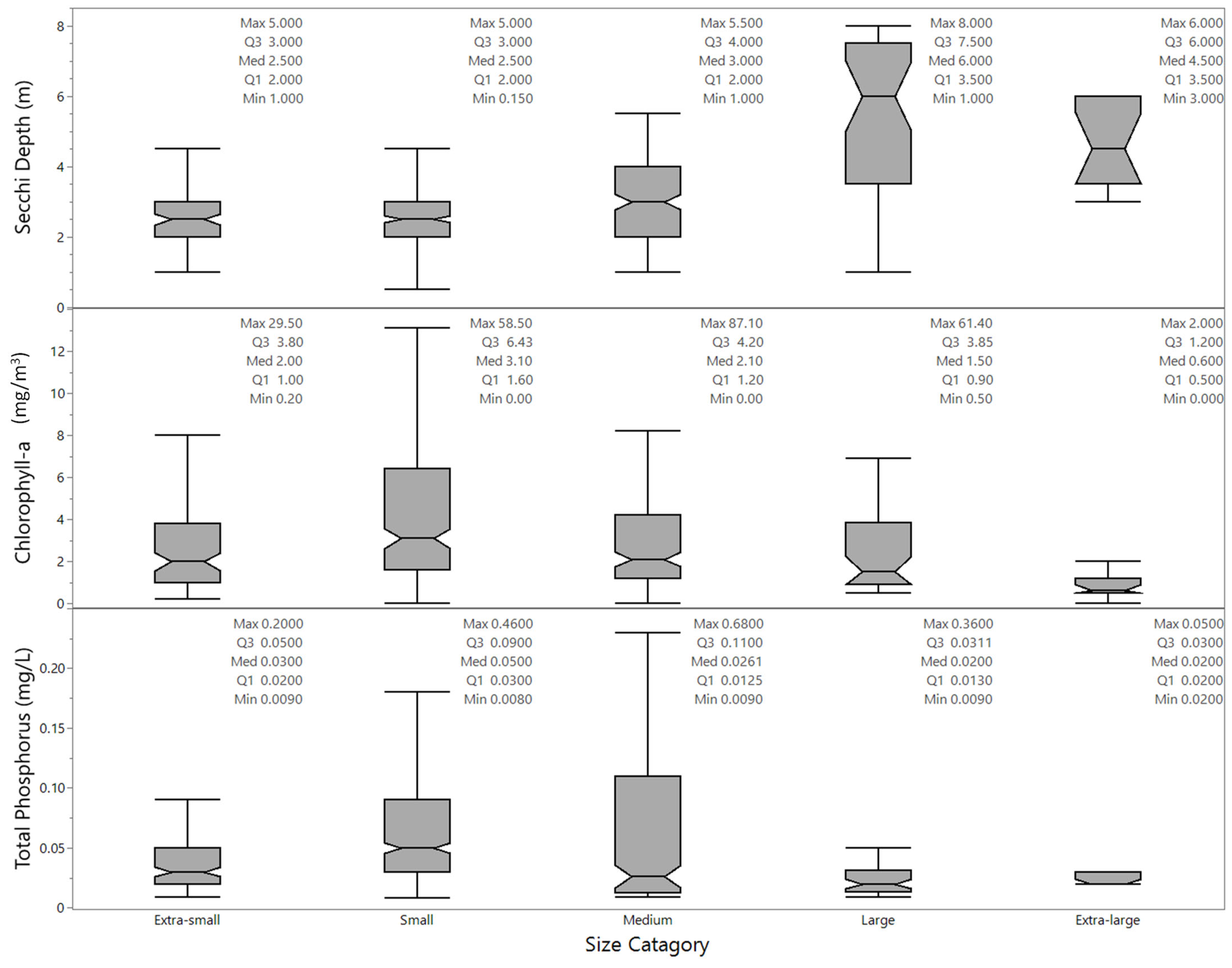
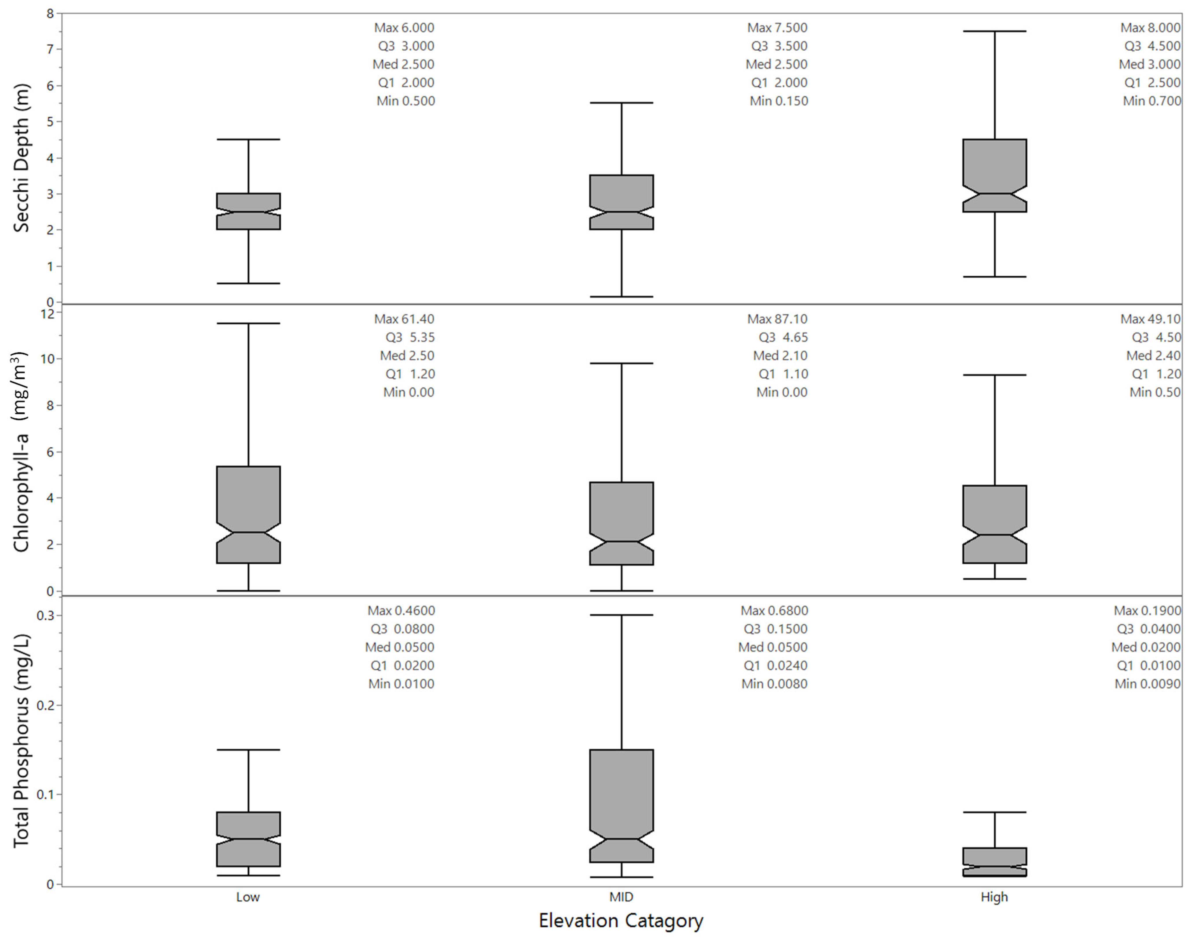
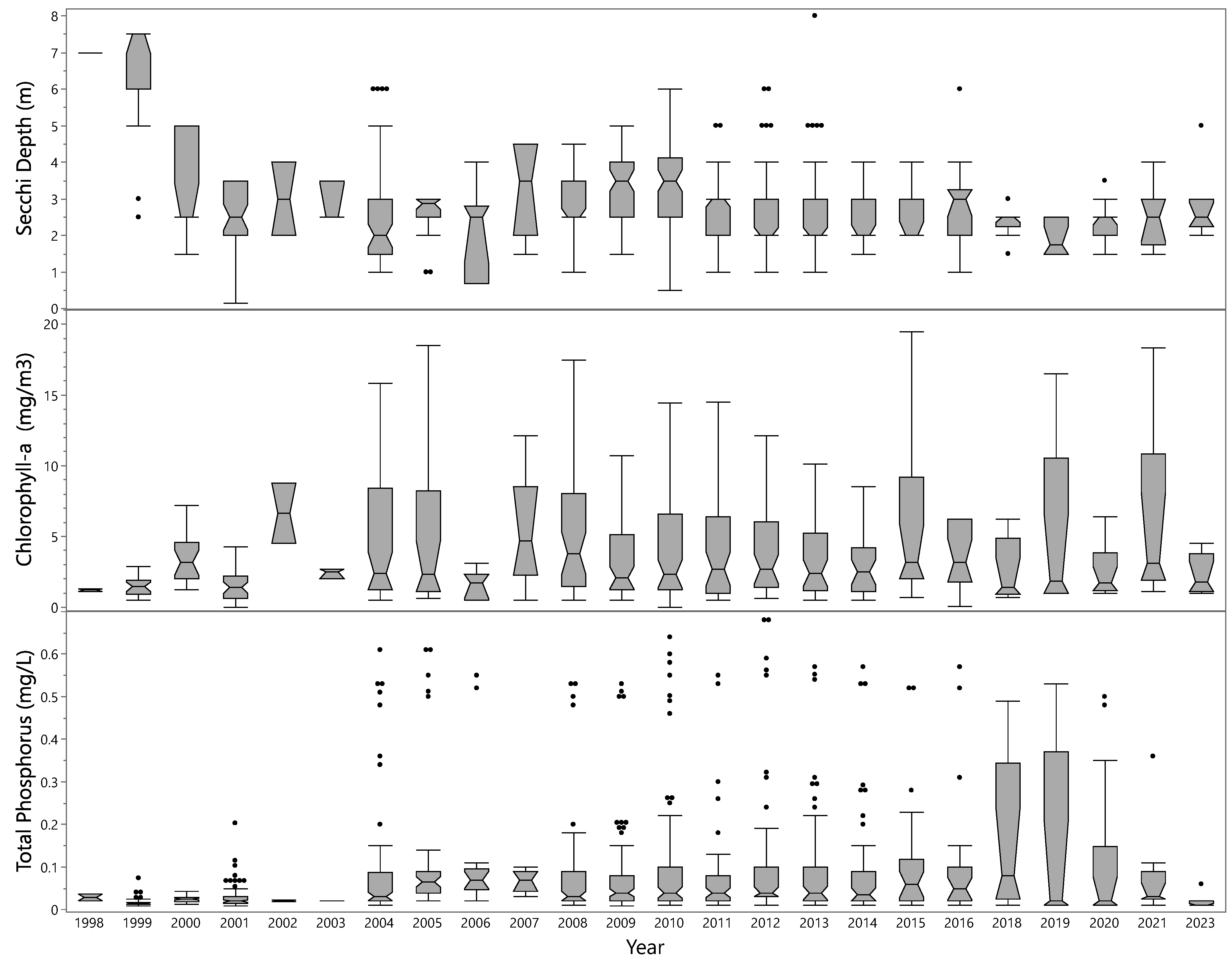
3.1.2. Data by Month, Lake Size, Elevation, and Year
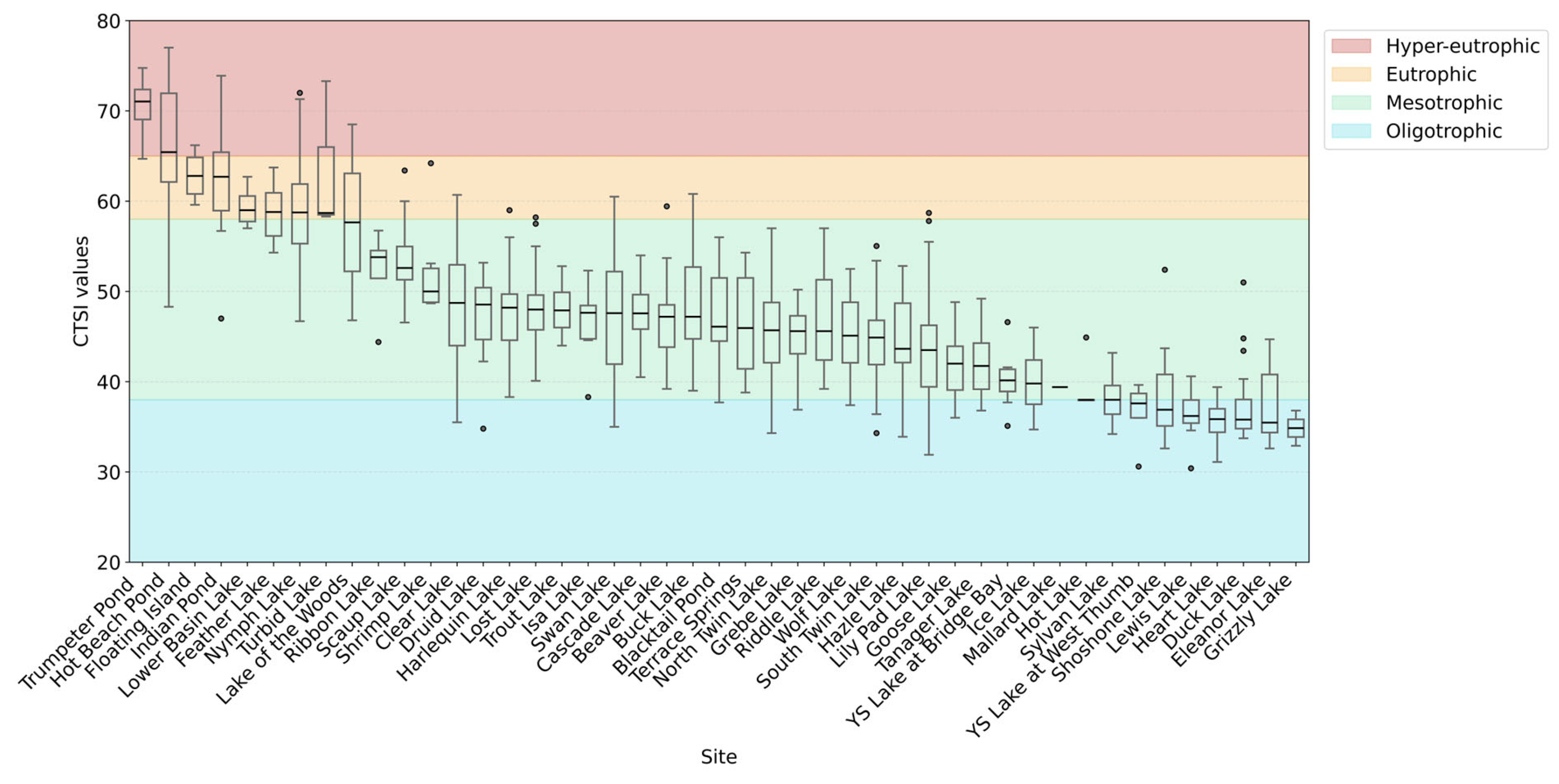
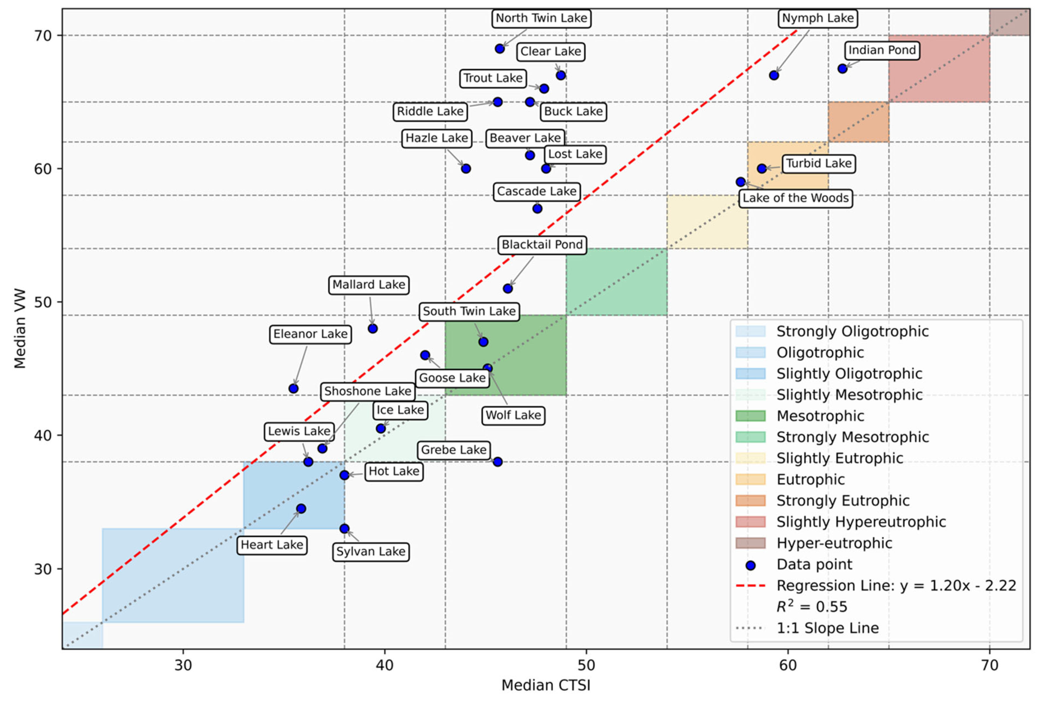
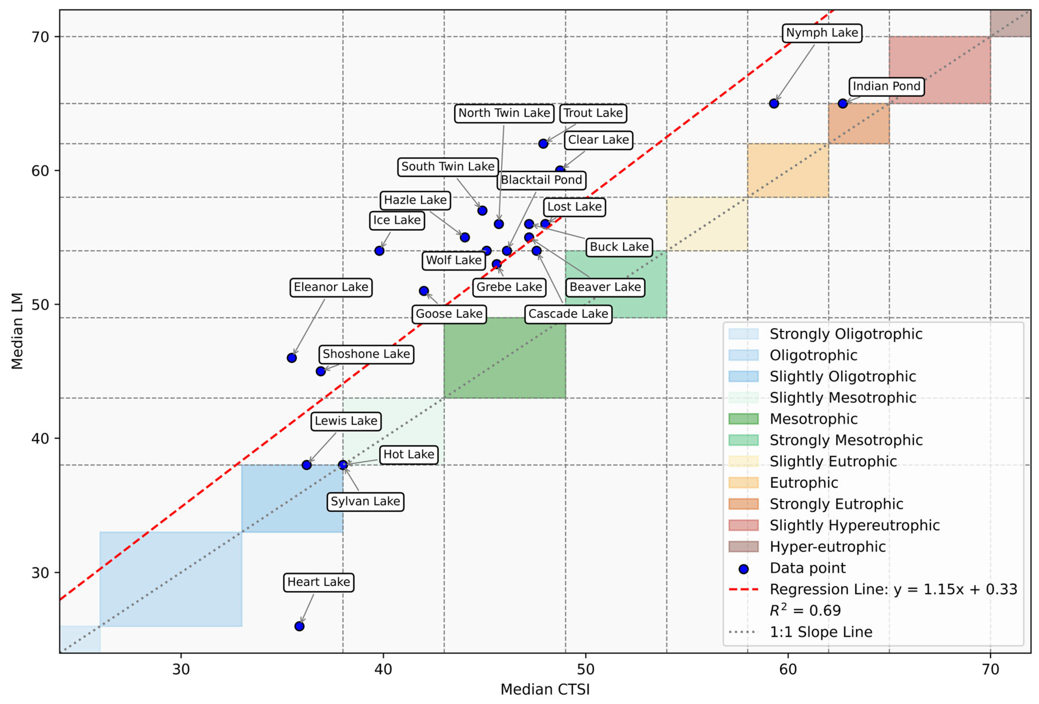
3.2. Trophic Model State and Comparison
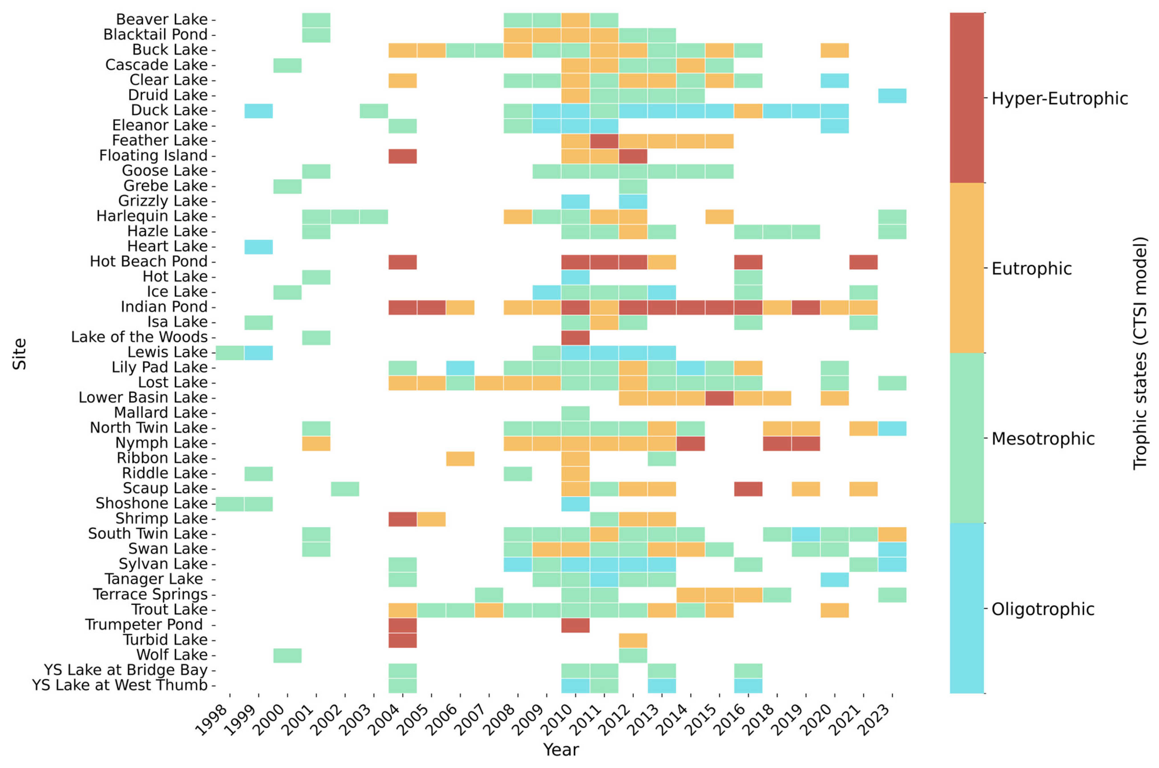
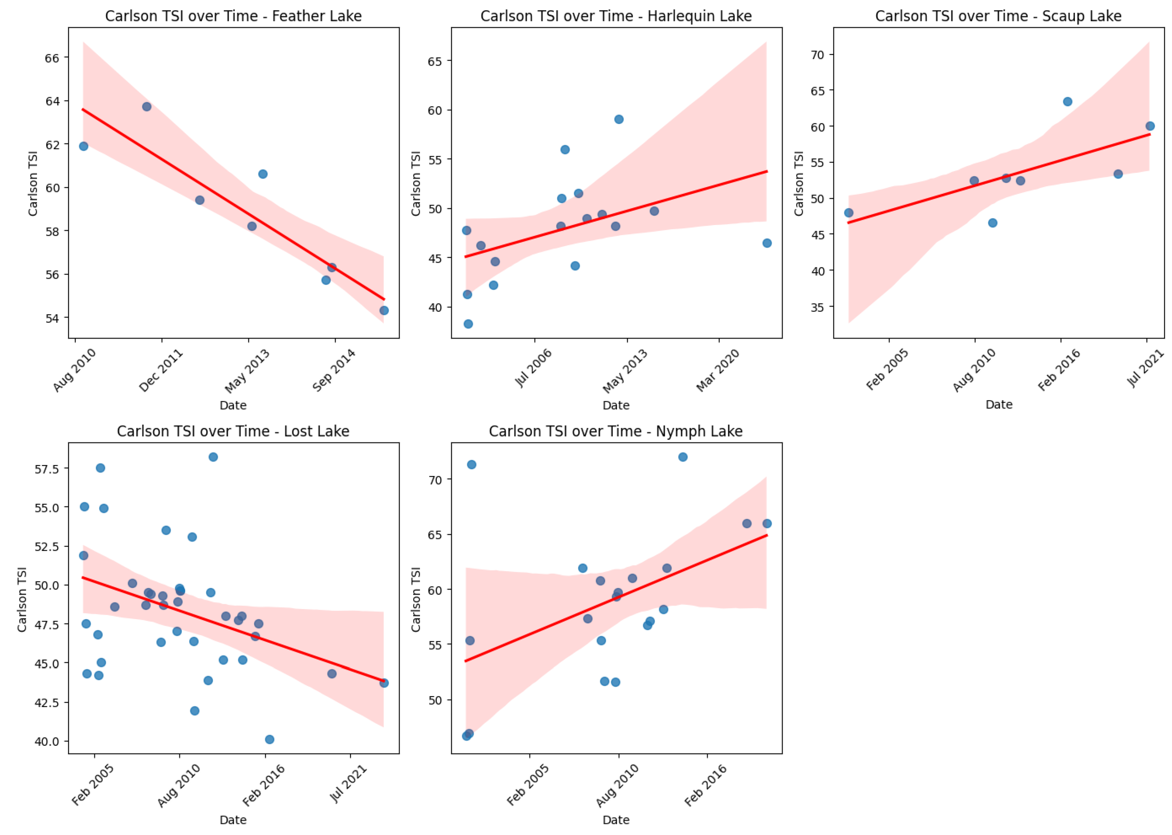
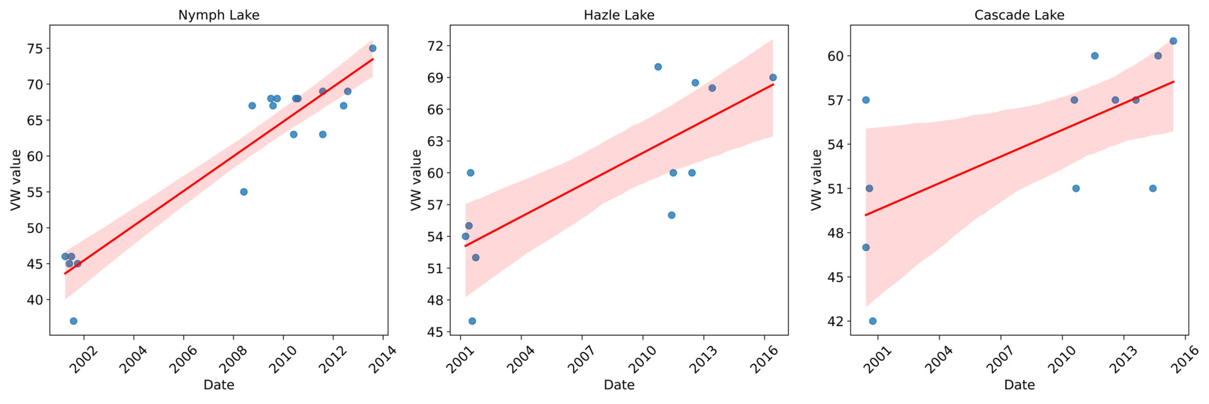
3.3. Time Series Analysis
3.3.1. Changes over Time
3.3.2. Mann–Kendall Results
4. Conclusions
Supplementary Materials
Author Contributions
Funding
Data Availability Statement
Acknowledgments
Conflicts of Interest
Abbreviations
| TSI | Trophic State Index |
| CTSI | Carlson Trophic State Index |
| VW | Vollenweider |
| LM | Larsen–Mercier |
| TP | Total Phosphorus |
| chl-a | Chlorophyll-a |
| SD | Secchi depth |
| HRT | Hydraulic Residence Time |
| PRC | Phosphorus Retention Coefficient |
| EPA | Environmental Protection Agency |
| MDPI | Multidisciplinary Digital Publishing Institute |
| SM10200 H | Standard Method 10200 H (used for chl-a analysis) |
| GEOGLOWS | Group on Earth Observations Global Water Sustainability |
| TDX-Hydro | TanDEM-X Hydro Elevation Model |
| DEM | Digital Elevation Model |
| NOAA | National Oceanic and Atmospheric Administration |
| PN | Pacific Northwest (in Bureau of Reclamation PN Regional Laboratory) |
Appendix A. VW Model Results


References
- Dudgeon, D.; Arthington, A.H.; Gessner, M.O.; Kawabata, Z.-I.; Knowler, D.J.; Lévêque, C.; Naiman, R.J.; Prieur-Richard, A.-H.; Soto, D.; Stiassny, M.L.J.; et al. Freshwater Biodiversity: Importance, Threats, Status and Conservation Challenges. Biol. Rev. 2006, 81, 163–182. [Google Scholar] [CrossRef] [PubMed]
- Izmailova, A.V.; Rumyantsev, V.A. Trophic Status of the Largest Freshwater Lakes in the World. Lakes Reserv. Sci. Policy Manag. Sustain. Use 2016, 21, 20–30. [Google Scholar] [CrossRef]
- Cardall, A.; Tanner, K.; Williams, G. Google Earth Engine Tools for Long-Term Spatiotemporal Monitoring of Chlorophyll-a Concentrations. Open Water J. 2021, 7, 4. [Google Scholar]
- Hansen, C.; Swain, N.; Munson, K.; Adjei, Z.; Williams, G.P.; Miller, W. Development of Sub-Seasonal Remote Sensing Chlorophyll-A Detection Models. Am. J. Plant Sci. 2013, 4, 21–26. [Google Scholar] [CrossRef]
- Hansen, C.H.; Burian, S.J.; Dennison, P.E.; Williams, G.P. Spatiotemporal Variability of Lake Water Quality in the Context of Remote Sensing Models. Remote Sens. 2017, 9, 409. [Google Scholar] [CrossRef]
- Hansen, C.H.; Williams, G.P.; Adjei, Z.; Barlow, A.; Nelson, E.J.; Woodruff Miller, A. Reservoir Water Quality Monitoring Using Remote Sensing with Seasonal Models: Case Study of Five Central-Utah Reservoirs. Lake Reserv. Manag. 2015, 31, 225–240. [Google Scholar] [CrossRef]
- Tanner, K.B.; Cardall, A.C.; Williams, G.P. A Spatial Long-Term Trend Analysis of Estimated Chlorophyll-a Concentrations in Utah Lake Using Earth Observation Data. Remote Sens. 2022, 14, 3664. [Google Scholar] [CrossRef]
- Bresciani, M.; Giardino, C.; Fabbretto, A.; Pellegrino, A.; Mangano, S.; Free, G.; Pinardi, M. Application of New Hyperspectral Sensors in the Remote Sensing of Aquatic Ecosystem Health: Exploiting PRISMA and DESIS for Four Italian Lakes. Resources 2022, 11, 8. [Google Scholar] [CrossRef]
- Taggart, J.B.; Ryan, R.L.; Williams, G.P.; Miller, A.W.; Valek, R.A.; Tanner, K.B.; Cardall, A.C. Historical Phosphorus Mass and Concentrations in Utah Lake: A Case Study with Implications for Nutrient Load Management in a Sorption-Dominated Shallow Lake. Water 2024, 16, 933. [Google Scholar] [CrossRef]
- Miller, A.W. Trophic State Evaluation for Selected Lakes in Yellowstone National Park, USA. WIT Trans. Ecol. Environ. 2010, 20, 143–155. [Google Scholar]
- STATS—Park Reports. Available online: https://irma.nps.gov/Stats/Reports/Park/YELL (accessed on 3 March 2025).
- News & Notes. Yellowstone Science; 2019. Volume 27 Issue 1: Vital Signs—Monitoring Yellowstone’s Ecosystem Health. Available online: https://www.nps.gov/subjects/yellowstonescience/yellowstone-science-archive.htm (accessed on 10 December 2024).
- Melcher, A.A. A Trophic State Analysis of Lakes in Yellowstone National Park; Brigham Young University: Provo, UT, USA, 2013. [Google Scholar]
- Smith, V.H. Eutrophication of Freshwater and Coastal Marine Ecosystems a Global Problem. Environ. Sci. Pollut. Res. 2003, 10, 126–139. [Google Scholar] [CrossRef] [PubMed]
- Khan, M.N.; Mohammad, F. Eutrophication: Challenges and Solutions. In Eutrophication: Causes, Consequences and Control; Ansari, A.A., Gill, S.S., Eds.; Springer: Dordrecht, The Netherlands, 2014; pp. 1–15. ISBN 978-94-007-7813-9. [Google Scholar]
- Ansari, A.A.; Singh Gill, S.; Lanza, G.R.; Rast, W. (Eds.) Eutrophication: Causes, Consequences and Control; Springer: Dordrecht, The Netherlands, 2011; ISBN 978-90-481-9624-1. [Google Scholar]
- Bhagowati, B.; Ahamad, K.U. A Review on Lake Eutrophication Dynamics and Recent Developments in Lake Modeling. Ecohydrol. Hydrobiol. 2019, 19, 155–166. [Google Scholar] [CrossRef]
- Dodds, W.K.; Bouska, W.W.; Eitzmann, J.L.; Pilger, T.J.; Pitts, K.L.; Riley, A.J.; Schloesser, J.T.; Thornbrugh, D.J. Eutrophication of U.S. Freshwaters: Analysis of Potential Economic Damages. Environ. Sci. Technol. 2009, 43, 12–19. [Google Scholar] [CrossRef] [PubMed]
- Grabow, W.O.K. Water and Health; EOLSS Publications: Abu Dhabi, United Arab Emirates, 2009; Volume 2, ISBN 978-1-84826-183-9. Available online: https://www.eolss.net/eolss-publications.aspx (accessed on 10 December 2024).
- Li, Y.; Shang, J.; Zhang, C.; Zhang, W.; Niu, L.; Wang, L.; Zhang, H. The Role of Freshwater Eutrophication in Greenhouse Gas Emissions: A Review. Sci. Total Environ. 2021, 768, 144582. [Google Scholar] [CrossRef]
- Smith, V.H.; Joye, S.B.; Howarth, R.W. Eutrophication of Freshwater and Marine Ecosystems. Limnol. Oceanogr. 2006, 51, 351–355. [Google Scholar] [CrossRef]
- Bennett, E.M.; Carpenter, S.R.; Caraco, N.F. Human Impact on Erodable Phosphorus and Eutrophication: A Global Perspective: Increasing Accumulation of Phosphorus in Soil Threatens Rivers, Lakes, and Coastal Oceans with Eutrophication. BioScience 2001, 51, 227–234. [Google Scholar] [CrossRef]
- Klippel, G.; Macêdo, R.L.; Branco, C.W.C. Comparison of Different Trophic State Indices Applied to Tropical Reservoirs. Lakes Reserv. Sci. Policy Manag. Sustain. Use 2020, 25, 214–229. [Google Scholar] [CrossRef]
- Zhang, Y.; Li, M.; Dong, J.; Yang, H.; Van Zwieten, L.; Lu, H.; Alshameri, A.; Zhan, Z.; Chen, X.; Jiang, X.; et al. A Critical Review of Methods for Analyzing Freshwater Eutrophication. Water 2021, 13, 225. [Google Scholar] [CrossRef]
- Cloutier, R.G.; Sanchez, M. Trophic Status Evaluation for 154 Lakes in Quebec, Canada: Monitoring and Recommendations. Water Qual. Res. J. 2007, 42, 252–268. [Google Scholar] [CrossRef]
- Saluja, R.; Garg, J.K. Trophic State Assessment of Bhindawas Lake, Haryana, India. Environ. Monit Assess. 2016, 189, 32. [Google Scholar] [CrossRef]
- Otiang’a-Owiti, G.E.; Oswe, I.A. Human Impact on Lake Ecosystems: The Case of Lake Naivasha, Kenya. Afr. J. Aquat. Sci. 2007, 32, 79–88. [Google Scholar] [CrossRef]
- Bachmann, R.W.; Jones, B.L.; Fox, D.D.; Hoyer, M.; Bull, L.A.; Canfield, D.E., Jr. Relations between Trophic State Indicators and Fish in Florida (USA) Lakes. Can. J. Fish. Aquat. Sci. 1996, 53, 842–855. [Google Scholar] [CrossRef]
- Carlson, R.E. A Trophic State Index for Lakes. Limnol. Oceanogr. 1977, 22, 361–369. [Google Scholar] [CrossRef]
- Vollenweider, R.A. Input-Output Models: With Special Reference to the Phosphorus Loading Concept in Limnology. Schweiz. Z. Hydrol. 1975, 37, 53–84. [Google Scholar] [CrossRef]
- Tapp, J.S. Eutrophication Analysis with Simple and Complex Models. J. Water Pollut. Control Fed. 1978, 50, 484–492. [Google Scholar]
- Lin, J.-L.; Karangan, A.; Huang, Y.M.; Kang, S.-F. Eutrophication Factor Analysis Using Carlson Trophic State Index (CTSI) towards Non-Algal Impact Reservoirs in Taiwan. Sustain. Environ. Res. 2022, 32, 25. [Google Scholar] [CrossRef]
- Moore, L.; Thornton, K. Lake and Reservoir Restoration Guidance Manual; North American Lake Management Society for US Environmental Protection Agency: Washington, DC, USA, 1988. [Google Scholar]
- Mann, H.B. Nonparametric Tests Against Trend. Econometrica 1945, 13, 245. [Google Scholar] [CrossRef]
- Donald, W.M.; Jean, S.; Steven, A.D.; Jon, B.H. Statistical Analysis for Monotonic Trends; Tech Notes 6, Developed for U.S. Environmental Protection Agency by Tetra Tech, Inc.; Tetra Tech, Inc.: Fairfax, VA, USA, 2011; 23p. Available online: https://www.epa.gov/sites/default/files/2016-05/documents/tech_notes_6_dec2013_trend.pdf (accessed on 10 December 2024).
- Roberts, W.; Williams, G.P.; Jackson, E.; Nelson, E.J.; Ames, D.P. Hydrostats: A Python Package for Characterizing Errors between Observed and Predicted Time Series. Hydrology 2018, 5, 66. [Google Scholar] [CrossRef]
- Jackson, E.K.; Roberts, W.; Nelsen, B.; Williams, G.P.; Nelson, E.J.; Ames, D.P. Introductory Overview: Error Metrics for Hydrologic Modelling—A Review of Common Practices and an Open Source Library to Facilitate Use and Adoption. Environ. Model. Softw. 2019, 119, 32–48. [Google Scholar] [CrossRef]


| Size (ha) | Classification |
|---|---|
| Area < 2 | Extra small |
| 2 ≤ Area < 10 | Small |
| 10 ≤ Area < 30 | Medium |
| 30 ≤ Area < 3000 | Large |
| Area ≥ 3000 | Extra large |
| Lake | Latitude | Longitude | Elevation (meters) | Est. Lake Area (ha) | Size Category | In-Lake Samples (Number) | Inlet Samples (Number) |
|---|---|---|---|---|---|---|---|
| Beaver Lake | −110.73 | 44.82 | 2243 | 0.63 | Extra small | 10 | 8 |
| Clear Lake | −110.48 | 44.71 | 2380 | 1.62 | 24 | 2 | |
| Eleanor Lake | −110.14 | 44.47 | 2588 | 1.70 | 13 | 5 | |
| Hazle Lake | −110.72 | 44.75 | 2282 | 1.92 | 16 | 12 | |
| Isa Lake | −110.72 | 44.44 | 2515 | 0.51 | 7 | NI * | |
| Lily Pad Lake | −111.01 | 44.17 | 2385 | 1.33 | 24 | NI | |
| Shrimp Lake | −110.13 | 44.91 | 2161 | 0.90 | 6 | NI | |
| Terrace Spring | −110.85 | 44.65 | 2098 | 0.58 | 8 | NI | |
| Blacktail Pond | −110.60 | 44.96 | 2014 | 5.67 | Small | 15 | 1 |
| Buck Lake | −110.13 | 44.90 | 2130 | 2.79 | 35 | 34 | |
| Druid Lake | −110.17 | 44.87 | 2038 | 3.85 | 10 | 0 | |
| Feather Lake | −110.84 | 44.54 | 2191 | 7.46 | 8 | 0 | |
| Floating Island | −110.45 | 44.94 | 2013 | 2.10 | 4 | NI | |
| Harlequin Lake | −110.89 | 44.64 | 2096 | 7.41 | 17 | NI | |
| Hot Lake | −110.79 | 44.54 | 2239 | 2.94 | 5 | 1 | |
| Lost Lake | −110.10 | 43.78 | 2086 | 5.26 | 38 | 16 | |
| Lower Basin Lake | −110.82 | 44.54 | 2201 | 4.14 | 12 | NI | |
| North Twin Lake | −110.74 | 44.78 | 2293 | 5.22 | 24 | 23 | |
| Nymph Lake | −110.73 | 44.75 | 2280 | 5.00 | 20 | 18 | |
| Ribbon Lake | −110.45 | 44.72 | 2381 | 3.86 | 4 | 0 | |
| Scaup Lake | −110.77 | 44.43 | 2404 | 2.26 | 8 | NI | |
| South Twin Lake | −110.73 | 44.77 | 2290 | 8.12 | 29 | 21 | |
| Trout Lake | −110.13 | 44.90 | 2124 | 6.36 | 37 | 34 | |
| Trumpeter Pond | −110.37 | 44.92 | 2066 | 4.68 | 4 | NI | |
| Cascade Lake | −110.52 | 44.75 | 2437 | 13.90 | Medium | 14 | 11 |
| Duck Lake | −110.58 | 44.42 | 2368 | 17.80 | 22 | NI | |
| Goose Lake | −110.84 | 44.54 | 2195 | 15.80 | 14 | 13 | |
| Hot Beach Pond | −110.30 | 44.55 | 2361 | 15.60 | 10 | NI | |
| Ice Lake | −110.63 | 44.72 | 2407 | 29.70 | 17 | 4 | |
| Indian Pond | −110.32 | 44.56 | 2366 | 12.00 | 48 | 23 | |
| Lake of the woods | −110.71 | 44.80 | 2356 | 11.20 | 2 | 1 | |
| Mallard Lake | −110.78 | 44.48 | 2443 | 13.00 | 1 | 1 | |
| Swan Lake | −110.74 | 44.92 | 2211 | 20.90 | 27 | NI | |
| Sylvan Lake | −110.16 | 44.48 | 2568 | 16.00 | 26 | 21 | |
| Tanager Lake | −110.69 | 44.14 | 2133 | 13.20 | 10 | NI | |
| Wolf Lake | −110.59 | 44.75 | 2442 | 20.20 | 5 | 3 | |
| Grebe Lake | −110.56 | 44.75 | 2450 | 62.80 | Large | 5 | 3 |
| Grizzly Lake | −110.77 | 44.81 | 2290 | 73.30 | 2 | 0 | |
| Heart Lake | −110.49 | 44.27 | 2282 | 993.00 | 4 | 2 | |
| Lewis Lake | −110.63 | 44.30 | 2374 | 1252.00 | 16 | 5 | |
| Riddle Lake | −110.55 | 44.36 | 2414 | 137.00 | 2 | 1 | |
| Shoshone Lake | −110.70 | 44.37 | 2380 | 2946.00 | 6 | 4 | |
| Turbid Lake | −110.27 | 44.56 | 2392 | 68.00 | 3 | 3 | |
| Yellowstone Lake (YSL@Bridge Bay) | −110.44 | 44.53 | 2357 | 3,5143.00 | Extra large | 8 | 0 |
| Yellowstone Lake (YSL@WestThumb) | −110.55 | 44.39 | 2357 | 3,5143.00 | 7 | 0 |
| Classification | Sub-Classification | Scale |
|---|---|---|
| Oligotrophic | Strongly oligotrophic | TSI < 26 |
| Oligotrophic | 26 ≤ TSI < 33 | |
| Slightly oligotrophic | 33 ≤ TSI < 38 | |
| Mesotrophic | Slightly mesotrophic | 38 ≤ TSI < 43 |
| Mesotrophic | 43 ≤ TSI < 49 | |
| Strongly mesotrophic | 49 ≤ TSI < 54 | |
| Eutrophic | Slightly eutrophic | 54 ≤ TSI < 58 |
| Eutrophic | 58 ≤ TSI < 62 | |
| Strongly eutrophic | 62 ≤ TSI < 65 | |
| Hyper-Eutrophic | Slightly hyper-eutrophic | 65 ≤ TSI < 70 |
| Hyper-eutrophic | 70 ≤ TSI |
| Statistic | Secchi Depth (m) | Chl-a (mg/m3) | TP (mg/L) |
|---|---|---|---|
| N | 635 | 620 | 916 |
| Mean | 2.904 | 4.923 | 0.081 |
| Std Dev | 1.287 | 8.103 | 0.125 |
| Std Err Mean | 0.051 | 0.325 | 0.004 |
| Upper 95% Mean | 3.005 | 5.562 | 0.089 |
| Lower 95% Mean | 2.804 | 4.284 | 0.073 |
| Skewness | 1.311 | 5.148 | 2.914 |
| Interquartile Range | 1.500 | 3.575 | 0.060 |
| Quantile | Name | Secchi Depth (m) | Chl-a (mg/m3) | TP (mg/L) |
|---|---|---|---|---|
| 100.0% | maximum | 8.000 | 87.100 | 0.680 |
| 99.5% | 7.500 | 61.095 | 0.610 | |
| 97.5% | 7.000 | 27.480 | 0.530 | |
| 90.0% | 4.500 | 11.460 | 0.190 | |
| 75.0% | quartile | 3.500 | 4.775 | 0.080 |
| 50.0% | median | 2.500 | 2.400 | 0.030 |
| 25.0% | quartile | 2.000 | 1.200 | 0.020 |
| 10.0% | 1.500 | 0.700 | 0.010 | |
| 2.5% | 1.000 | 0.500 | 0.010 | |
| 0.5% | 0.536 | 0.000 | 0.009 | |
| 0.0% | minimum | 0.150 | 0.000 | 0.008 |
| Site Location | CTSI | VW | LM |
|---|---|---|---|
| Beaver Lake | Mesotrophic | Slightly eutrophic | Slightly eutrophic |
| Blacktail Pond | Mesotrophic | Strongly mesotrophic | Slightly eutrophic |
| Buck Lake | Mesotrophic | Slightly hyper-eutrophic | Slightly eutrophic |
| Cascade Lake | Mesotrophic | Slightly eutrophic | Slightly eutrophic |
| Clear Lake | Mesotrophic | Slightly hyper-eutrophic | Eutrophic |
| Druid Lake | Mesotrophic | ||
| Duck Lake | Slightly oligotrophic | ||
| Eleanor Lake | Slightly oligotrophic | Mesotrophic | Mesotrophic |
| Feather Lake | Eutrophic | ||
| Floating Island | Strongly eutrophic | ||
| Goose Lake | Slightly mesotrophic | Mesotrophic | Strongly mesotrophic |
| Grebe Lake | Mesotrophic | Slightly mesotrophic | Strongly mesotrophic |
| Grizzly Lake | Slightly oligotrophic | ||
| Harlequin Lake | Mesotrophic | ||
| Hazle Lake | Mesotrophic | Eutrophic | Slightly eutrophic |
| Heart Lake | Slightly oligotrophic | Slightly oligotrophic | Slightly oligotrophic |
| Hot Beach Pond | Strongly eutrophic | ||
| Hot Lake | Slightly mesotrophic | Slightly oligotrophic | Slightly mesotrophic |
| Ice Lake | Slightly mesotrophic | Slightly mesotrophic | Slightly eutrophic |
| Indian Pond | Strongly eutrophic | Slightly hyper-eutrophic | Slightly hyper-eutrophic |
| Isa Lake | Mesotrophic | ||
| Lake of the woods | Slightly eutrophic | Eutrophic | |
| Lewis Lake | Slightly oligotrophic | Slightly mesotrophic | Slightly mesotrophic |
| Lily Pad Lake | Mesotrophic | ||
| Lost Lake | Mesotrophic | Slightly eutrophic | Slightly eutrophic |
| Lower Basin Lake | Eutrophic | ||
| Mallard Lake | Slightly mesotrophic | Mesotrophic | |
| North Twin Lake | Mesotrophic | Slightly hyper-eutrophic | Slightly eutrophic |
| Nymph Lake | Eutrophic | Eutrophic | Slightly hyper-eutrophic |
| Ribbon Lake | Strongly mesotrophic | ||
| Riddle Lake | Mesotrophic | Strongly eutrophic | |
| Scaup Lake | Strongly mesotrophic | ||
| Shoshone Lake | Slightly mesotrophic | Slightly mesotrophic | Mesotrophic |
| Shrimp Lake | Strongly mesotrophic | ||
| South Twin Lake | Mesotrophic | Mesotrophic | Slightly eutrophic |
| Swan Lake | Mesotrophic | ||
| Sylvan Lake | Slightly mesotrophic | Slightly mesotrophic | Slightly mesotrophic |
| Tanager Lake | Slightly mesotrophic | ||
| Terrace Springs | Mesotrophic | ||
| Trout Lake | Mesotrophic | Slightly hyper-eutrophic | Eutrophic |
| Trumpeter Pond | Hyper-eutrophic | ||
| Turbid Lake | Strongly eutrophic | Eutrophic | |
| Wolf Lake | Mesotrophic | Mesotrophic | Strongly mesotrophic |
| YSL [Bridge Bay] | Slightly mesotrophic | ||
| YSL [West Thumb] | Slightly oligotrophic |
| Lake | CTSI | Chl-a (In-Lake) | TP (In-Lake) | VW (Inlet) | TP (Inlet) | PRC (Inlet) |
|---|---|---|---|---|---|---|
| Blacktail Pond | Increasing | |||||
| Cascade Lake | Increasing | Increasing | Increasing | |||
| Buck Lake | Decreasing | |||||
| Feather Lake | Decreasing | Decreasing | Decreasing | |||
| Harlequin Lake | Increasing | Increasing | ||||
| Hazel Lake | Increasing | Increasing | Increasing | |||
| Lewis Lake | Decreasing | |||||
| Lost Lake | Decreasing | |||||
| North Twin Lake | Increasing | |||||
| Nymph Lake | Increasing | Increasing | Increasing | Increasing | ||
| Scaup Lake | Increasing |
Disclaimer/Publisher’s Note: The statements, opinions and data contained in all publications are solely those of the individual author(s) and contributor(s) and not of MDPI and/or the editor(s). MDPI and/or the editor(s) disclaim responsibility for any injury to people or property resulting from any ideas, methods, instructions or products referred to in the content. |
© 2025 by the authors. Licensee MDPI, Basel, Switzerland. This article is an open access article distributed under the terms and conditions of the Creative Commons Attribution (CC BY) license (https://creativecommons.org/licenses/by/4.0/).
Share and Cite
Miller, A.W.; P. Williams, G.; Magoffin, R.H.; Li, X.; Miskin, T.; Aghababaei, A.; Wagle, P.; Chapagain, A.R.; Baaniya, Y.; Oldham, P.D.; et al. Trophic State Evolution of 45 Yellowstone Lakes over Two Decades: Field Data and a Longitudinal Study. Water 2025, 17, 1627. https://doi.org/10.3390/w17111627
Miller AW, P. Williams G, Magoffin RH, Li X, Miskin T, Aghababaei A, Wagle P, Chapagain AR, Baaniya Y, Oldham PD, et al. Trophic State Evolution of 45 Yellowstone Lakes over Two Decades: Field Data and a Longitudinal Study. Water. 2025; 17(11):1627. https://doi.org/10.3390/w17111627
Chicago/Turabian StyleMiller, A. Woodruff, Gustavious P. Williams, Rachel Huber Magoffin, Xueyi Li, Taylor Miskin, Amin Aghababaei, Pitamber Wagle, Abin Raj Chapagain, Yubin Baaniya, Peter D. Oldham, and et al. 2025. "Trophic State Evolution of 45 Yellowstone Lakes over Two Decades: Field Data and a Longitudinal Study" Water 17, no. 11: 1627. https://doi.org/10.3390/w17111627
APA StyleMiller, A. W., P. Williams, G., Magoffin, R. H., Li, X., Miskin, T., Aghababaei, A., Wagle, P., Chapagain, A. R., Baaniya, Y., Oldham, P. D., Oldham, S. J., Peterson, T., Prince, L., Tanner, K. B., Cardall, A. C., & Ames, D. P. (2025). Trophic State Evolution of 45 Yellowstone Lakes over Two Decades: Field Data and a Longitudinal Study. Water, 17(11), 1627. https://doi.org/10.3390/w17111627