Abstract
The water hammer phenomenon, characterized by transient pressure surges due to rapid fluid deceleration in pipelines, poses significant risks to hydraulic systems. Valve closure time is a critical parameter influencing pressure magnitude, necessitating precise calibration to ensure system safety. While numerical methods like the MacCormack scheme provide accurate solutions, their computational intensity limits practical applications. This study addresses this limitation by proposing a machine learning (ML) framework employing a multilayer perceptron (MLP) artificial neural network (ANN) to predict optimal pressure values—defined as the lowest maximum pressure obtained for several closure laws at a given closure time—corresponding to specific valve closure times. The ANN was trained on 637 simulations generated via the MacCormack method, which solves the hyperbolic partial differential equations governing transient flow in a reservoir-pipeline-valve (RPV) system. Performance evaluation metrics demonstrate the ANN’s exceptional robustness and accuracy, achieving a root mean square error (RMSE) of 0.068, Nash-Sutcliffe efficiency (NSE) of 0.99, and a correlation coefficient (R) of 0.99, with a maximum relative error below 1%. The results highlight the ANN’s superior predictive accuracy and flexibility in capturing complex transient flow dynamics, outperforming conventional numerical methods. Notably, the ANN reduced computational time from days for iterative simulations to mere seconds, enabling rapid prediction of pressure-time curves critical for real-time decision-making. This framework offers a computationally efficient and reliable alternative for optimizing valve closure strategies, mitigating water hammer risks, and enhancing pipeline safety. By bridging numerical rigor with machine learning, this work enhances hydraulic infrastructure resilience across industrial and urban networks.
1. Introduction
Transient flows in pipeline systems, arising from abrupt disruptions to steady-state conditions such as valve closures or pump operations, induce dangerous pressure surges termed water hammer. These phenomena jeopardize infrastructure integrity, necessitating robust predictive and mitigation strategies. The study of unsteady flows traces back to foundational work by Lagrange (1788) [1], who formulated wave propagation principles for compressible and incompressible flows. Building on this, Monge (1789) [2] introduced the method of characteristics for solving hyperbolic partial differential equations, a cornerstone for transient flow analysis. Bergeron (1931) [3] later expanded this framework, establishing analytical relationships between pressure and velocity in pipelines. A pivotal advancement came with Joukowsky (1904) [4], whose simplified water hammer formula remains central to modern transient flow studies. Building on these foundations, Wylie et al. (1993) [5] pioneered the valve stroking technique, strategically modulating closure patterns to dampen pressure surges, which became a cornerstone for later advancements in transient flow control.
Contemporary research has focused on optimizing valve closure strategies to mitigate extreme pressures. Twyman (2018a) [6] emphasized gradual valve closure as a protective measure, while Yong et al. (2022) [7] demonstrated how valve type and closure laws influence peak pressures. Bazargan et al. (2013) [8] advanced this field by integrating Bayesian networks with multi-objective optimization to derive optimal closure rules. Complementary approaches include valve trajectory calibration via impedance and particle swarm methods (Sanghyun, 2019) [9], hybrid mechanical solutions combining flywheels and check valves (Bettaieb & Haj Taieb, 2020) [10], and fluid-structure interaction models assessing pipe material effects (Yu et al., 2022) [11]. Recent numerical innovations, such as the MacCormack method [12], have further refined valve closure laws to minimize overpressure and depression.
Despite these advances, traditional numerical methods remain computationally intensive, limiting real-time applications. This study bridges the gap by employing artificial neural networks (ANNs) to predict optimal pressure values during transient flow in sloped pipelines. By training ANNs on a dataset generated via the MacCormack method, the approach circumvents iterative simulations, enabling rapid and precise predictions tailored to varying valve closure times.
The paper is structured as follows: First, the governing equations for transient flow are presented. Second, the MacCormack numerical scheme is detailed, including boundary condition handling. Third, ANN architectures are systematically evaluated to identify optimal configurations for pressure prediction. Finally, results are discussed, emphasizing the model’s accuracy and its potential to enhance real-time decision-making in hydraulic systems. This work bridges machine learning and hydraulic engineering, offering a scalable tool for pipeline safety and efficiency.
2. Mathematical Model and Resolution Methods
2.1. Mathematical Model
The fundamental hyperbolic equations that accurately describe transient flow phenomena in a hydraulic pipeline are sequentially derived from the continuity and momentum equations and are given by system (1): [13].
This system relates piezometric head (H) and flow rate (Q) variations over time and space, considering wave velocity (a), friction losses (j), pipe cross-section (S), and pipe inclination (α). For buried pipes, wave velocity is calculated using standard formulas [13], and head loss per unit length is given by Darcy-Weisbach [14]. The MacCormack method, a finite difference scheme, was employed to solve these equations, involving predictor and corrector steps [15]. Boundary conditions were handled using quadratic interpolation. Additionally, an artificial neural network (ANN), specifically a multilayer perceptron (MLP), was developed to predict transient pressures. Trained on MacCormack-generated data, the MLP uses back-propagation with Levenberg-Marquardt optimization, evaluated via the quadratic loss function [16].
2.2. Resolution of the Transient Flow Problem by the MacCormack Method
The MacCormack method is one of the most popular discretizations for hyperbolic partial differential equations. It operates in two stages: In the forecasting step, an upstream-weighted finite difference approach is applied; during the correction step, a finite difference method skewed downstream is applied. These steps are mathematically summarized as follows:
- Predictor step:
- Corrector step:
Applying these two steps to the system of equations number seven leads to the following expressions:
- Predictor step: This step allows the prediction of the values of H and Q at time (t + Δt). The results of applying this step are represented in the following equations:
With:
- Corrector step: This step allows the correction of the values of H and Q at time (t + Δt) obtained in the prediction step. So, applying this step gives the following equations:
With:
Δt: time step; Δx: space step; i: space index; k: time index; : average flow rate between nodes (i + 1) and (i − 1) at time t; the quantities; , , , and denote the flow rate and the piezometric head at time t and at time t + Δt, respectively [14].
The application of the diagram of the MacCormack method to the interior nodes will not cause any problems, but at the boundary limits (on the left and on the right), it results in the following expressions:
At node i = 1
Only the correction step presents a problem at this node, where the flow rate is represented in the following form:
- Corrector step
At node i = N
At this node, the problem arises only in the prediction step, and the expression giving the piezometric head is written as follows:
- Predictor step
The two formulas explicitly illustrate the emergence of two fictitious nodes, i = 0 and i = N + 1, with coordinates successively (Q0, H0) and (QN+1,HN+1). For this purpose, the values of flow rate and pressure head at the nodes (i = 1) and (i = N) are determined using quadratic interpolation.
At the first node (node number 1), the fictitious point (0) arises only for the hydraulic parameter Q, and at the last node (node number N), the fictitious point (N + 1) arises only for the hydraulic parameter H, and whose objective is to get rid of these two fictitious points, Second-Order Lagrange Polynomial is used to obtain expressions giving Q(1) and H(N). The results obtained using this polynomial are as follows:
At the first node i = 1
At the last node (i = N),
2.3. Solving the Transient Flow Problem Using the (ANN)
Before delving into the second method for analyzing transient flow, it’s worth clarifying two concepts: artificial neural networks (ANNs) and formal neurons. ANNs mimic the human brain’s functionality through software-based artificial neurons. A formal neuron, in turn, is a nonlinear, bounded algebraic function. Its output depends on weighted inputs, which act as coefficients (see Figure 1). These input variables define the neuron as a mathematical operator with calculable numerical values. Figure 1 shows how the weighted sum of input predictors is processed using a parameterized function with set limits. The final output of the neuron is then calculated in Equation (10).
where a’ is the neuron’s output, f is the transfer function, R is the number of inputs, b is the bias of neuron 1, and w1j is the weight enclosing neuron 1 and input pj.
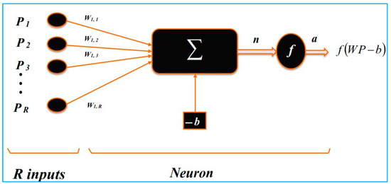
Figure 1.
Mathematical model of a formal neuron.
The term topology or architecture describes the arrangement and connections of neurons in a neural network. At the level of the neurons themselves, we rather talk about the neighborhood, which refers to how a neuron is connected to other neurons.
The neighborhood of a neuron, which represents all the neurons connected to it, is directly linked to the network architecture.
Taking a closer look at the meaning of the term neighborhood in the context of neural network architecture, it refers to the neurons connected to a given neuron. The neighborhood of order n for neuron i means that there are n other neurons connected to it.
In artificial neural networks, there are various types of structures, which are distinguished by the way in which the neurons are interconnected. Among these types of structures, we can cite the following: Neural network with recurrent connections, fully connected neural network, Kohonen network, and Multilayer Perceptron (MLP) neural network.
The most commonly used architecture in artificial neural networks is the multilayer perceptron (MLP) topology [17]. In this type of architecture, neurons are organized in layers. The input information is transmitted from layer to layer until the output result is obtained [18,19]. In this topology, neurons are divided into three categories: input neurons, hidden neurons, and output neurons.
In artificial neural networks, the multilayer perceptron architecture is simply an extension of probably the most widely used single-layer perceptron topology, shown in Figure 2a.
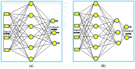
Figure 2.
Architecture of perceptron-type neural networks. (a) Single-layer perceptron and (b) the multi-layer perceptron with two hidden layers.
In a multiple-layer artificial neural network, the neurons are organized into distinct layers, and each of them transmits information connected to all neurons in the previous and next layers, excepting the neural connections in the input layer and the output layer. There are no direct connections between neurons of the same layer (Figure 2b). Such an architecture allows neural networks to trace complex relationships between input and output data, hence making them very powerful tools in the solution of nonlinearly separable problems and complex logical problems [20].
This topology is widely used to solve prediction problems like our problem seeking to predict the values of the optimal pressure during the genesis of the transient flow.
The MLP is a type of feedforward network containing a minimum of three distinct layers: input, hidden, and output. Each neuron conveys information by transmitting signals between consecutive layers. Learning is a crucial process in neural networks, where the algorithm uses desired input-output data pairs in supervised learning that are used to refine network parameters, such as weights and biases. MLP learning is supervised and based on the back-propagation algorithm, which improves network performance by reducing the squared error of the loss function between simulated and calculated results [16,21,22]. The Quadratic Loss Function (QLF) for N training samples is given by Equation (11):
where si and ci are the simulated and calculated values for the ith training sample, respectively. According to Özkal et al. (2022) [16], the Levenberg-Marquardt method is particularly robust and efficient. In this paper, we base our method to carry out the learning of our ANN.
3. Problem Statement and Boundary Conditions
3.1. Problem Statement
To illustrate the mathematical model derived, the RPV (Reservoir—Pipeline—Valve) system is adopted (Figure 3). This system comprises a large reservoir positioned at the upstream section of the inclined pipeline and a valve situated at the downstream end that discharges into the atmosphere. The reservoir, with an overflow at an elevation designated Hr, delivers a flow rate Q0 through a gravity pipe with a length labelled L and characterized by thickness e, diameter d, and roughness ε, inclined at an angle α°. At the opposite end of the pipeline, there is a motorized valve with controlled closure located at a height called Hvl. The transient flow is generated by a closing process of the valve. The schematic representation of the problem is depicted in Figure 3.
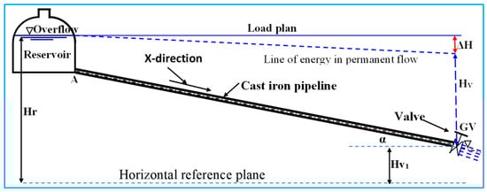
Figure 3.
Reservoir-Pipeline-Valve System Schematic.
3.2. Boundary Conditions and Stability Criterion
When applying the MacCormack method using finite differences, undefined variables appear at the limits (on the left and on the right) of the domain of interest. This section highlights how to eliminate this indeterminacy.
3.2.1. At the Outlet of the Reservoir
The piezometric head at the first node (pipe entrance) is equal to the piezometric height of the water in the reservoir represented by H(1) = Hr. The expression number (8) is used to calculate the flow rate.
3.2.2. At the Valve
In the scenario of instantaneous closure (valve closing time equals zero), Q(n) = 0, the piezometric head at node N can be expressed using Equation (9) mentioned earlier. While the closure is controlled, the flow at the valve varies over time according to a function defined by the selected closing law. The flow in this instance can be described as a function of Q0, Δt, Ct, and m using the equation that follows [23,24]:
With,
m: Exponent determining the valve closing law;
Ct: The total valve closing time;
Qk and Qk+1 are successively the flow rates at times t and t + Δt.
Figure 4 illustrates the variation in flow over time for different possible closing valve laws (for different values of m).
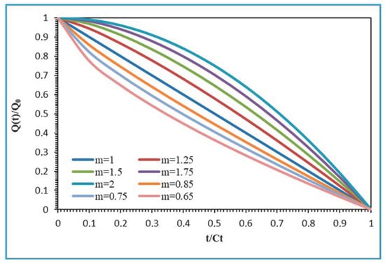
Figure 4.
Temporal flow changes corresponding to various valve closure laws.
The exponent m of the expression of Q at node n generates an infinity of functions of Q, and consequently, the search for the optimal value of this exponent turns out to be a major priority for optimal management.
The stability criterion of the MacCormack method is satisfied when the following expression is verified [6,7]:
To rigorously minimize numerical dispersion and adhere to the Courant-Friedrichs-Lewy (CFL) condition, the Courant number (C = aΔt/Δx) was enforced at unity (C = 1) by selecting the time step as Δt = Δx/a, ensuring both stability and accuracy in the MacCormack simulations [25,26].
4. Results and Discussions
4.1. Database Creation
Optimizing hydraulic parameters in transient flow systems through numerical methods often requires iterative simulations, a computationally intensive and time-consuming process for identifying ideal values. To overcome these computational hurdles and improve efficiency, we propose a two-stage approach. First, we developed a comprehensive database encompassing all variables involved in simulation and optimization. Second, we systematically analyzed relationships between input parameters and target outcomes. When selecting a model, it is critical to account for all quantities influencing hydraulic characteristics in both transient and steady-state flows. Given the large number of variables, we reduced complexity by grouping interrelated parameters and retaining only essential independent variables. These quantities are divided into inlet and outlet quantities, where the thickness, roughness, diameter, slope, and length of the pipe; the hydraulic load on the reservoir; the level and the closing time of the valve are input quantities, and the optimal pressure and the piezometric head are output quantities.
Table 1 presents some values of the vectors from the created database containing 637 rows. In this database, we have targeted the values of the optimal pressure calculated by a code in the Fortran language, allowing us to solve the two transient flow equations by the MacCormack method, to simulate the hydraulic parameters in transient flow, and to accurately follow the pressure variations at all discretization nodes along the pipe. This code not only enables real-time monitoring of pressure evolution but also determines the maximum pressure values for a wide range of valve closure times and closure laws. For each closure time, we plotted the maximum pressure obtained as a function of the closure laws used. Each resulting curve exhibits a distinct minimum value, which is referred to as the optimal pressure.

Table 1.
Input and target quantities created.
Table 2 has been drawn up to give an overall statistical idea of the input and output parameters.
Table 2.
Statistical results of the database obtained.
The statistical analysis of this table highlights a significant variability in hydraulic and geometric parameters. Pipe diameters and lengths vary significantly (0.04 m to 2 m and 50 m to 2000 m, respectively), directly impacting flow behavior. The flow rate shows high dispersion (CV = 1.43), ranging from 0.95 L/s to 4710 L/s, reflecting a broad spectrum of flow conditions. Similarly, roughness varies considerably (0.0074 mm to 2.335 mm) with a CV of 2.11. The inclination angle reaches 90°, suggesting vastly different pipeline configurations. The valve level also shows notable variation, ranging from 0 m to 284 m, impacting pressure regulation within the system. Additionally, the valve closing time fluctuates between 0.27 s and 88.99 s (CV = 1.10), highlighting significant differences in operational control strategies. Finally, the optimal pressure fluctuates between 2.06 bars and 47.99 bars, while the reservoir head ranges from 25 m to 500 m, demonstrating a wide operational range despite a moderate variability (CV ≈ 0.38).
In this phase of our study, we focus on employing artificial neural networks (ANNs) to identify the most reliable model architecture for predicting optimal pressure under these heterogeneous conditions.
4.2. Database Utilization and ANN Architecture Optimization for Pressure Prediction
In this part of this paper, we will use the database input and output vectors created as vectors of the calculated values. This database was divided into three separate sets to adjust the ANN architecture parameters to obtain the best performance. Seventy percent of the data was allocated for the training phase, 15% for validation, and the remaining 15% for testing across the various ANN structures. Figure 5 shows the ANN model diagram.
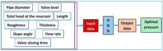
Figure 5.
ANN model diagram.
A total of 19 different structures were processed by the ANN to evaluate and compare these structures in terms of performance in order to opt for the best architecture of the ANNs. This is based on the results of Hecht-Nielsen (1987) [27]. who determined the number of neurons in the hidden layer using the formula 2i + 1, where i is the number of Wu model inputs [28]. Since i is equal to 9 in our scenario, the buried layer’s maximum number of neurons is equal to 19.
Finding the right number of neurons in the hidden layer for the database’s input and output vectors is the crucial step in this section. This step was carried out by testing the RMSE and the relative maximum error by varying the number of hidden neurons. This consists of starting with 1 neuron in the hidden layer, then increasing this number of 1 neuron up to 19. Subsequently, the architecture offering the first best possible performance will be chosen based on the validation and test results. Figure 6 elucidates the search flowchart for the architecture with the best performance.
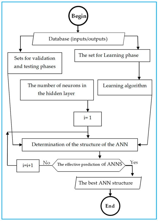
Figure 6.
Flowchart explaining the development of ANNs.
4.3. Choice of Performance Evaluation Criteria
The assessment of the ANN structure’s performance often relies on the simulation of the error between the values predicted by the ANN and the calculated values.
The validation of the ANN model relies on statistical parameters throughout the training, validation, and testing phases.
The correlation coefficient (R). the Nash-Sutcliffe efficiency coefficient (NSE). and the root-mean-square error (RMSE) are the three metrics employed in this study to evaluate the efficacy of the ANN structure [29,30].
where: Pti is the calculated value of the optimal pressure; is the value of the optimal pressure simulated by the model; is the average value of the calculated optimal pressure; is the average value of the optimal pressure simulated by the model; and N is the amount of data. The results obtained from RMSE, NSE, and R are mentioned in Table 3.
Table 3.
Statistical results of the ANN structure in the training, validation, and testing phases.
The statistical results further demonstrate that the architecture composed of 15 neurons in the hidden layer gives the best performance, and therefore this structure is chosen to carry out the simulation calculations of the optimal pressure by the ANN. This architecture (15 hidden neurons) achieved exceptional accuracy across all phases (Table 4). During testing, the model yielded RMSE = 0.068, NSE = 0.99, and R = 0.99, with a maximum relative error of 0.98%.
Table 4.
Statistical results of optimal architecture (15 neurons).
Notably, the ANN has significantly reduced calculation time compared to conventional MacCormack simulations, enabling real-time pressure prediction. These results underscore the ANN’s potential to replace iterative methods in operational settings where rapid decision-making is critical. The results of the statistical parameters of this architecture are mentioned in Table 4.
To illustrate the architectures of the ANN examined during the learning, validation, and testing phases, the RMSE and the maximum relative error are plotted as a function of the number of neurons in the hidden layer. The RMSE results of the three phases and the maximum relative error obtained are shown in Figure 7 and Figure 8.
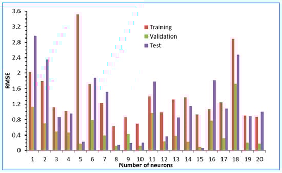
Figure 7.
Variation in RMSE depending on the number of neurons in the learning, validation, and test phases.
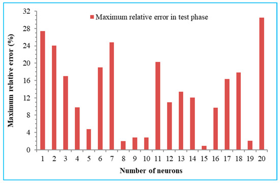
Figure 8.
Maximum relative error as a function of the number of neurons in the hidden layer in the test phase.
During the training phase, the number of neurons in the hidden layer that yields the lowest RMSE value is 10, with a corresponding value of 0.6873.
The maximum value of the relative error in the test phase is also taken in this study since a value of the maximum error exceeding 1% can make. In this type of flow, the calculated results are inaccurate. The expression for the maximum relative error (Er max) is written as follows:
In the validation and testing phases. The number of neurons in the hidden layer giving low RMSE and relative maximum error values is equal to 15.
Figure 9 shows the calculated and simulated values of the optimal pressure and the Nash-Sutcliffe efficiency coefficient (NSE) in the training, Validation, and test phases.
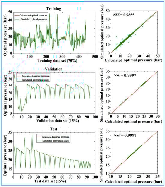
Figure 9.
Calculated and simulated values of optimal pressure and NSE in training, validation, and test phases.
The search for optimal pressure values is done according to the closing time of the valve. since each closing time has its own optimal pressure value. Figure 10 shows the variation over time of the calculated and simulated values of the optimal pressure for the optimal structure composed of 15 neurons in the hidden layer in the test phase.
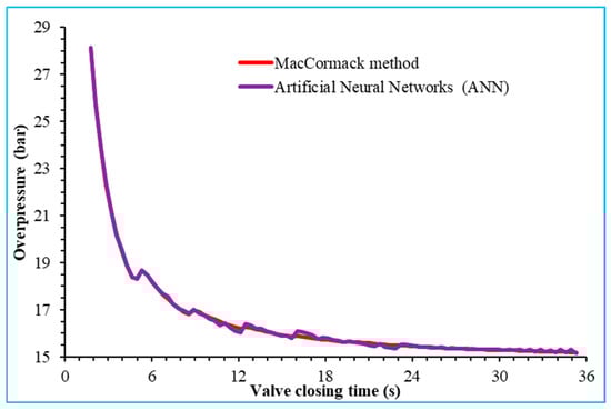
Figure 10.
Variation over time of the calculated and simulated values of the optimal overpressure for a number of neurons in the hidden layer equal to 15 in the test phase.
Figure 10 demonstrates a strong correlation between calculated and simulated values. the maximum relative error of which does not exceed 1%.
The use of ANN to predict the values of the optimal pressure in transient flow saves time and precision and offers a modern technique that could lead to the development and growth of complex phenomena such as transient flow, which is characterized by a change in their parameters over time.
5. Conclusions
This study demonstrates the transformative potential of artificial neural networks (ANNs) in addressing the water hammer phenomenon. By training a multilayer perceptron (MLP) ANN on 637 high-fidelity simulations derived from the MacCormack method, we achieved remarkable accuracy (RMSE = 0.068, NSE = 0.99, R = 0.99) in predicting optimal pressures during valve closure. The ANN’s predictive accuracy and flexibility outperform traditional numerical approaches, effectively capturing complex transient flow dynamics governed by hyperbolic partial differential equations.
A key innovation lies in the ANN’s computational efficiency. While conventional simulations required days to generate pressure-time curves, the ANN delivers results within seconds, enabling rapid optimization of valve closure strategies. This drastic reduction in computation time-from days to seconds-empowers engineers to implement real-time safety protocols and integrate the framework into supervisory control systems (e.g., SCADA) for dynamic transient analysis.
The model’s robustness is validated across diverse hydraulic conditions, including variable pipe geometries (0.04–2 m diameters, 0–90° slopes) and closure times (0.27–88.99 s), ensuring generalizability to real-world scenarios. Statistical validation confirmed maximum relative errors below 1%, surpassing Bayesian and impedance-based methods. By prioritizing accuracy without sacrificing efficiency, this work establishes ANNs as a benchmark for transient flow analysis, offering a scalable solution to safeguard hydraulic infrastructure against water hammer risks.
Author Contributions
Writing—original draft preparation. F.A. and A.T.; writing—review and editing. F.A., Z.A. and A.T.; data analysis. Z.A., A.T. and F.A.; software. Z.A., F.A. and A.T.; study design and conceptualization. A.T., F.A. and F.S.; validation. Z.A. and A.T.; supervision. A.T. and F.S. All authors have read and agreed to the published version of the manuscript.
Funding
This research received no external funding.
Data Availability Statement
All data are included in the paper.
Conflicts of Interest
The remaining authors declare that the research was conducted in the absence of any commercial or financial relationships that could be construed as a potential conflicts of interest.
References
- Lagrange, J.L. Méchanique Analytique; La Veuve Desaint: Paris, France, 1788. [Google Scholar]
- Wood, F. History of Water-Hammer; Queen’s University: Kingston, ON, Canada, 1970. [Google Scholar]
- Bergeron, L. Variation de Régime dans les Conduites d’eau; Comptes rendus des travaux de la Société hydrotechnique de France; Société hydrotechnique de France: Paris, France, 1931. [Google Scholar]
- Joukowsky, N. On the hydraulic hammer in water supply pipe. Proc. Am. Water Work. Assoc. 1904, 24, 341–424. [Google Scholar]
- Wylie, E.B.; Streeter, V.L.; Suo, L. Fluid Transients in Systems; Prentice Hall: Englewood Cliffs, NJ, USA, 1993. [Google Scholar]
- Twyman, J. Water hammer in a pipe network due to a fast valve closure. Rev. Ing. Constr. 2018, 33, 193–200. [Google Scholar] [CrossRef]
- Han, Y.; Shi, W.; Xu, H.; Wang, J.; Zhou, L. Effects of closing times and laws on water hammer in a ball valve pipeline. Water 2022, 14, 1497. [Google Scholar] [CrossRef]
- Bazargan-Lari, M.R.; Kerachian, R.; Afshar, H.; Bashi-Azghadi, S.N. Developing an optimal valve closing rule curve for real-time pressure control in pipes. J. Mech. Sci. Technol. 2013, 27, 215–225. [Google Scholar] [CrossRef]
- Sanghyun, K. Valve Maneuver Prediction in Simple and Complicated Pipeline Systems. Water Resour. Manag. 2019, 33, 4671–4685. [Google Scholar]
- Bettaieb, N.; Haj Taieb, E. Assessment of Failure Modes Caused by Water Hammer and Investigation of Convenient Control Measures. J. Pipeline Syst. Eng. Pract. 2020, 11, 04020006. [Google Scholar] [CrossRef]
- Chen, Y.; Zhao, C.; Guo, Q.; Zhou, J.; Feng, Y.; Xu, K. Fluid-Structure Interaction in a Pipeline Embedded in Concrete During Water Hammer. Front. Energy Res. 2022, 10. [Google Scholar] [CrossRef]
- Abdelouaheb, T.; Fateh, S.; Afoufou, F. Transient Flow in Pressurized Pipes: A Comparative Study of Five Resolution Methods. J. Civ. Eng. 2024, 19. [Google Scholar] [CrossRef]
- Streeter, V.L.; Wylie, E.B. Fluid Mechanics; McGraw-Hill: Ann Arbor, MI, USA, 1983; 206p. [Google Scholar]
- Neyestanaki, M.K.; Dunca, G.; Jonsson, P.; Cervantes, M.J. A Comparison of Different Methods for Modelling Water Hammer Valve Closure with CFD. Water 2023, 15, 1510. [Google Scholar] [CrossRef]
- Moser, A.P. Buried Pipe Design, 2nd ed.; McGraw-Hill: Ann Arbor, MI, USA, 2001. [Google Scholar]
- Özkal, İ.; Özkan, İ.A.; Başçiftçi, F. Metaverse token price forecasting using artificial neural networks (ANNs) and Adaptive neural fuzzy inference system (ANFIS). Neural Comput. Applic. 2024, 36, 3267–3290. [Google Scholar] [CrossRef]
- Van Hilten, A.; Katz, S.; Saccenti, E.; Niessen, W.J.; Roshchupkin, G.V. Designing interpretable deep learning applications for functional genomics: A quantitative analysis. Brief. Bioinform. 2024, 25, bbae449. [Google Scholar] [CrossRef] [PubMed]
- Najjar, Y.; Ali, H. On the use of BPNN in liquefaction potential assessment tasks. Artificial Intelligence and Mathematical Methods in Pavement and Geomechanical Systems. Attoh-Okine 1998, 75, 55–63. [Google Scholar]
- Najjar, Y.; Zhang, X.C. Characterizing the 3D stress-strain behavior of sandy soils: A neuro-mechanistic approach. In Numerical Methods in Geotechnical Engineering; American Society of Civil Engineers: Reston, VA, USA, 2000; pp. 43–57. [Google Scholar]
- Riad, S.; Mania, J.; Bouchaou, L.; Najjar, Y. Predicting catchment flow in a semi-arid region via an artificial neural network technique. Hydrol. Process. 2004, 18, 2387–2393. [Google Scholar] [CrossRef]
- Santos, C.A.; Freire, P.K.; Silva, R.M.D.; Akrami, S.A. Hybrid wavelet neural network approach for daily inflow forecasting using tropical rainfall measuring mission data. J. Hydrol. Eng. 2019, 24, 04018062. [Google Scholar] [CrossRef]
- Poonia, V.; Tiwari, H.L. Rainfall-runoff modeling for the Hoshangabad Basin of Narmada River using artificial neural network. Arab. J. Geosci. 2020, 13, 944. [Google Scholar] [CrossRef]
- Provenzano, P.G.; Baroni, F.; Aguerre, R.J. The closing function in the water hammer modeling. Lat. Am. Appl. Res. 2011, 41, 43–47. [Google Scholar]
- Subani, N.; Norsarahaida, A. Analysis of Water Hammer with Different Closing Valve Laws on Transient Flow of Hydrogen-Natural Gas Mixture. Hindawi Publishing Corporation. In Abstract and Applied Analysis; Hindawi Publishing Corporation: London, UK, 2015; p. 510675. [Google Scholar]
- Shampine, L.F. Two-step Lax–Friedrichs method. Appl. Math. Lett. 2005, 18, 1134–1136. [Google Scholar] [CrossRef]
- Goldberg, D.E.; Benjamin, W.E. Characteristics method using time-line interpolations. J. Hydraul. Eng. 1983, 109, 670–683. [Google Scholar] [CrossRef]
- Hecht-Nielsen, R. Kolmogorov’s mapping neural network existence theorem. In Proceedings of the First IEEE International Conference on Neural Networks, San Diego, CA, USA, 21–24 June 1987; pp. 11–14. [Google Scholar]
- Wu, G.D.; Lo, S.L. Predicting real-time coagulant dosage in water treatment by artificial neural networks and adaptive network-based fuzzy inference system. Eng. Appl. Artif. Intell. 2008, 21, 1189–1195. [Google Scholar] [CrossRef]
- Benchaiba, L.; Moussouni, A.; Zeghmar, A.; Maaliou, A. Wavelet and AI-based reservoir evaporation modeling for optimized water management: A case study of Koudiat Acerdoun Dam. Theor. Appl. Climatol. 2025, 156, 219. [Google Scholar] [CrossRef]
- Parmar, K.S.; Bhardwaj, R. River Water Prediction Modeling Using Neural Networks, Fuzzy and Wavelet Coupled Model. Water Resour. Manag. 2015, 29, 17–33. [Google Scholar] [CrossRef]
Disclaimer/Publisher’s Note: The statements, opinions and data contained in all publications are solely those of the individual author(s) and contributor(s) and not of MDPI and/or the editor(s). MDPI and/or the editor(s) disclaim responsibility for any injury to people or property resulting from any ideas, methods, instructions or products referred to in the content. |
© 2025 by the authors. Licensee MDPI, Basel, Switzerland. This article is an open access article distributed under the terms and conditions of the Creative Commons Attribution (CC BY) license (https://creativecommons.org/licenses/by/4.0/).