
Water Balance Estimates and Piezometric Level Lowering Based on Numerical Modeling and Remote Sensing Data in the Recife Metropolitan Region—Pernambuco (Brazil)

Abstract
1. Introduction
2. Materials and Methods
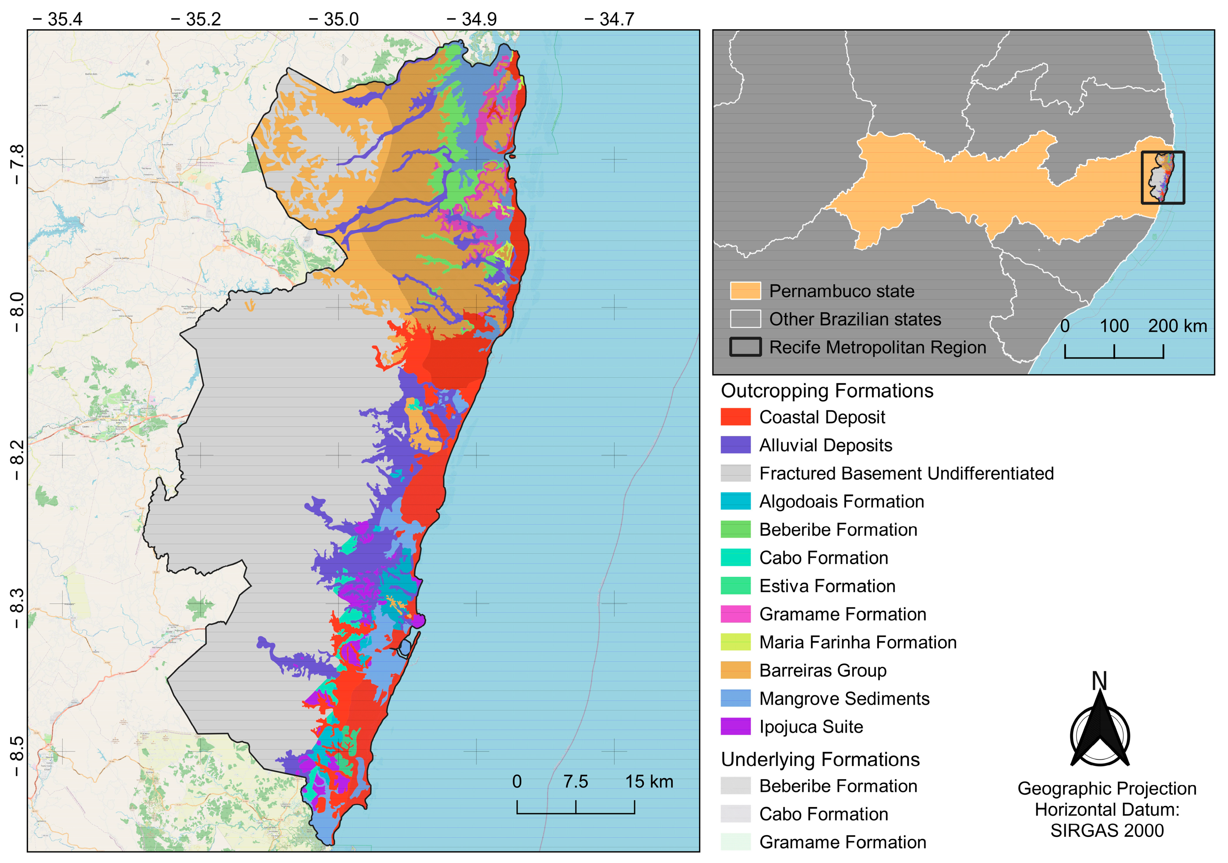
2.1. Geological and Hydrogeological Characterization of the Study Area
2.2. Conceptual Model
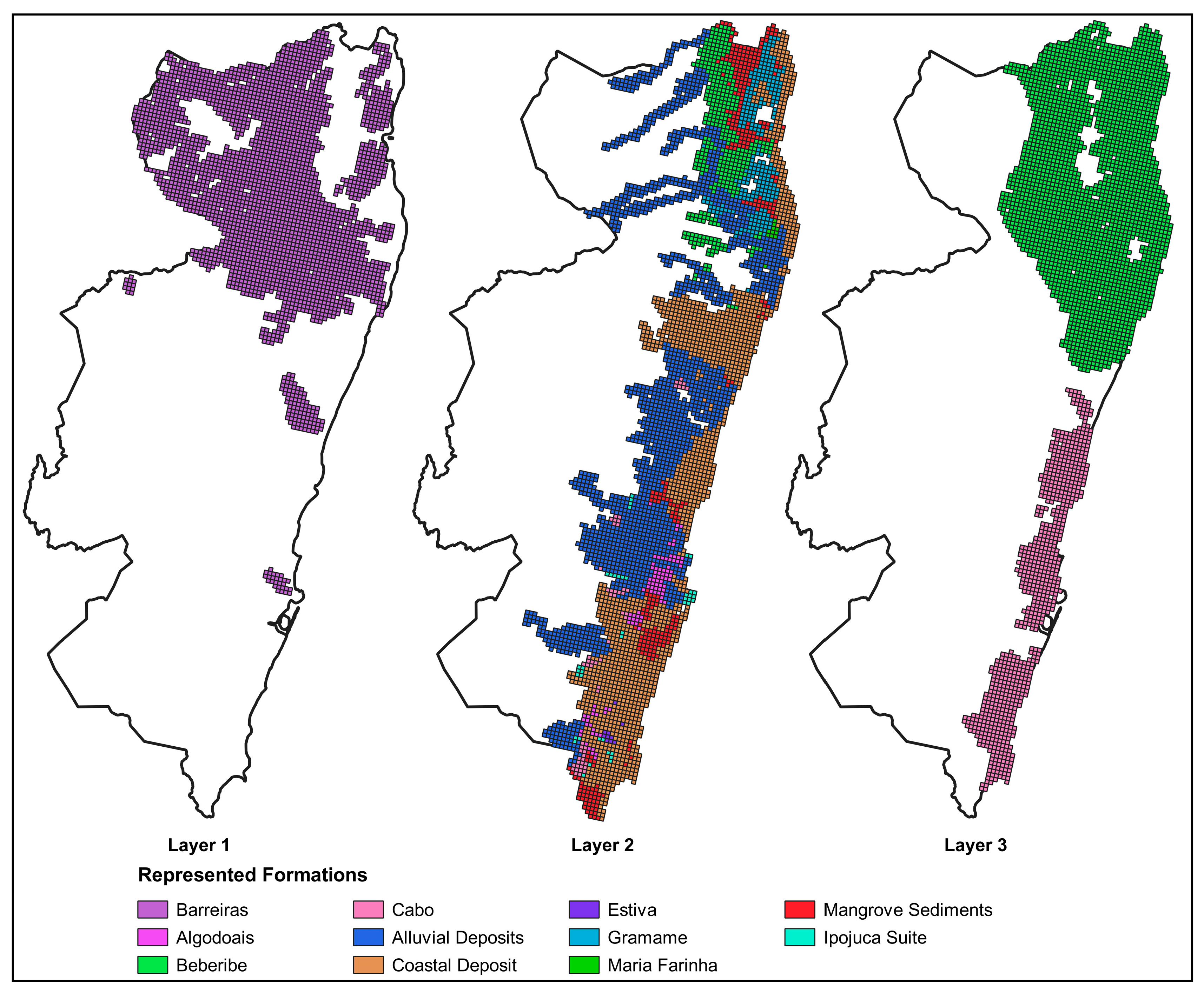
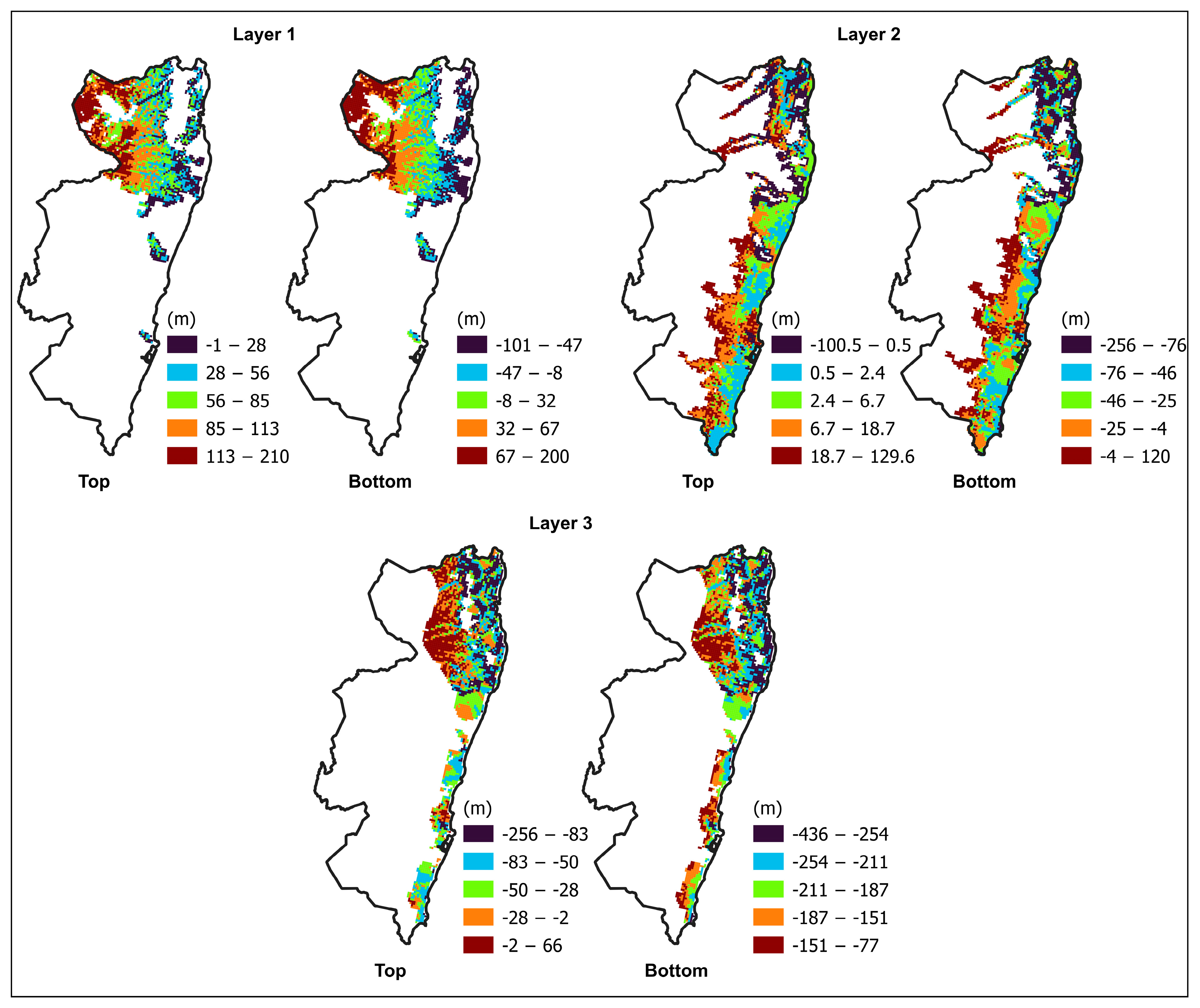
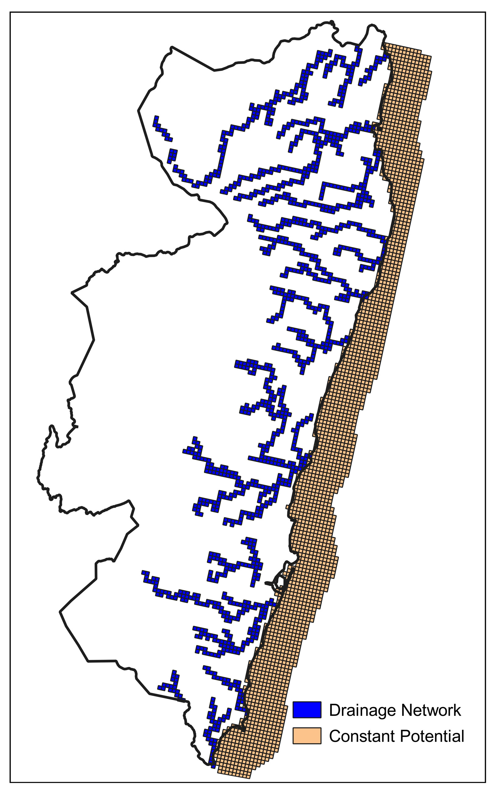
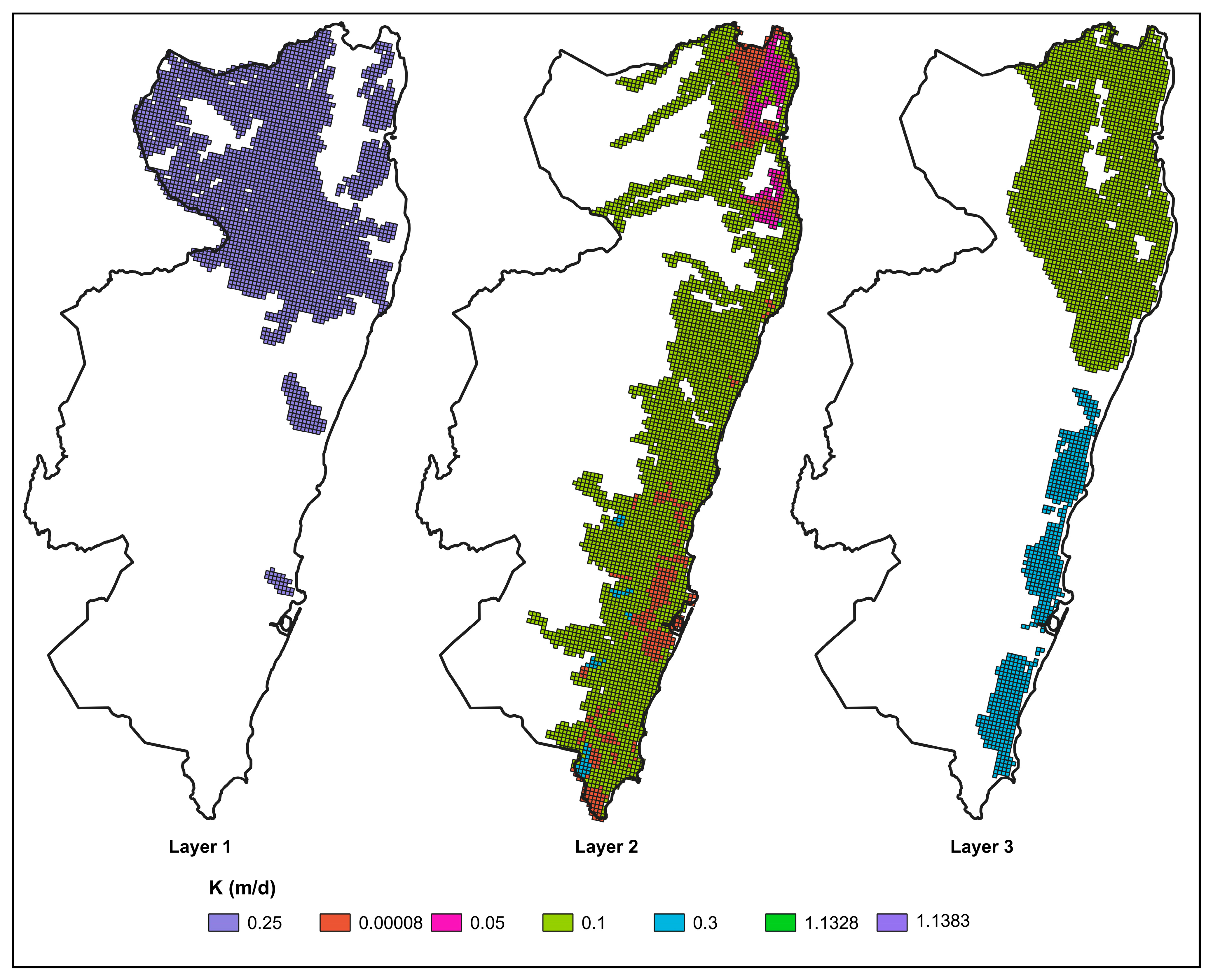
2.3. Numerical Model
2.4. Model Evaluation Statistics
3. Results and Discussion
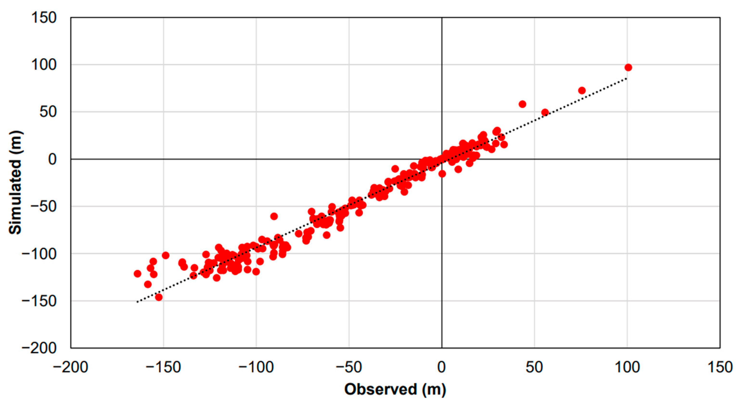
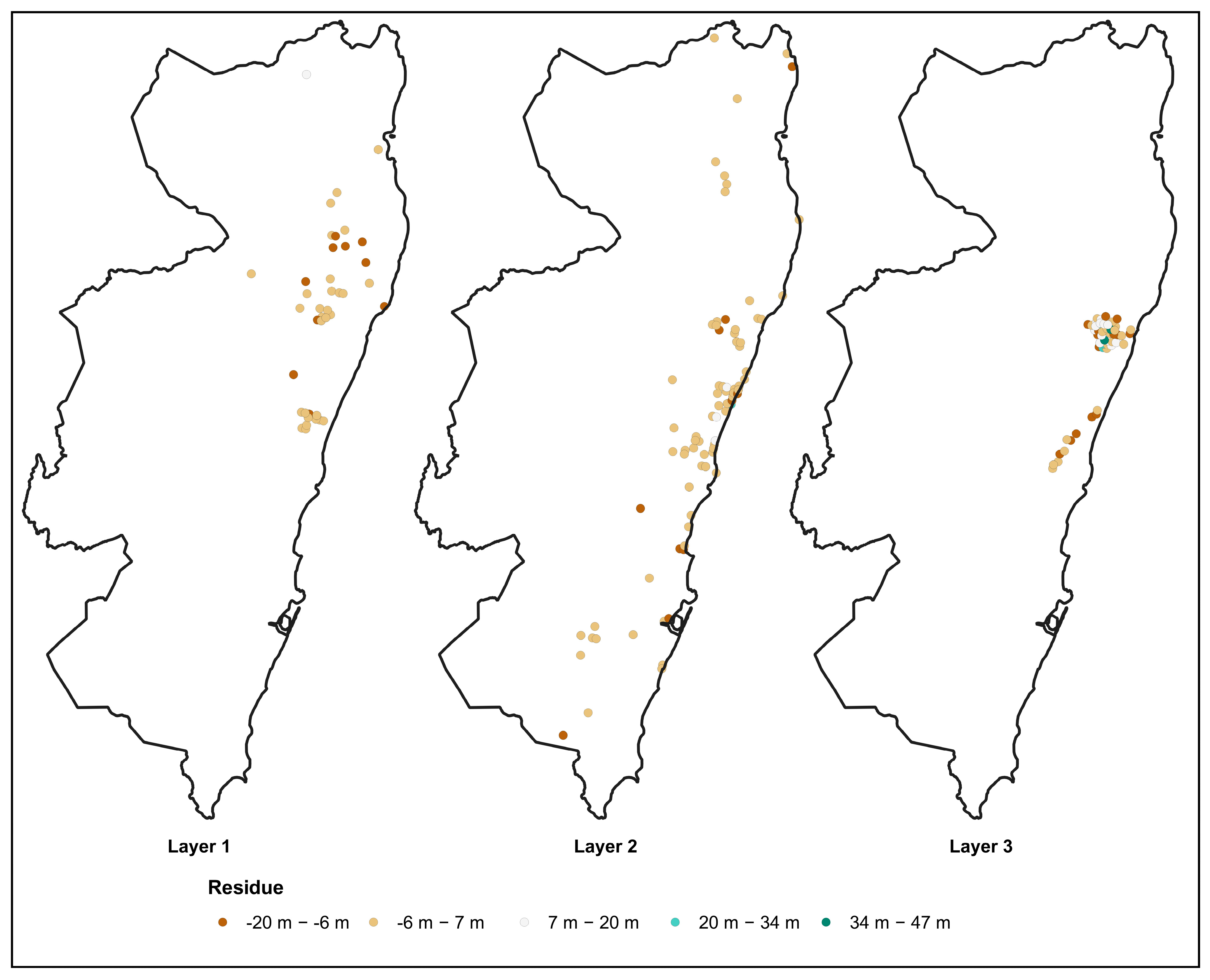
3.1. Model Calibration
3.2. Water Balance
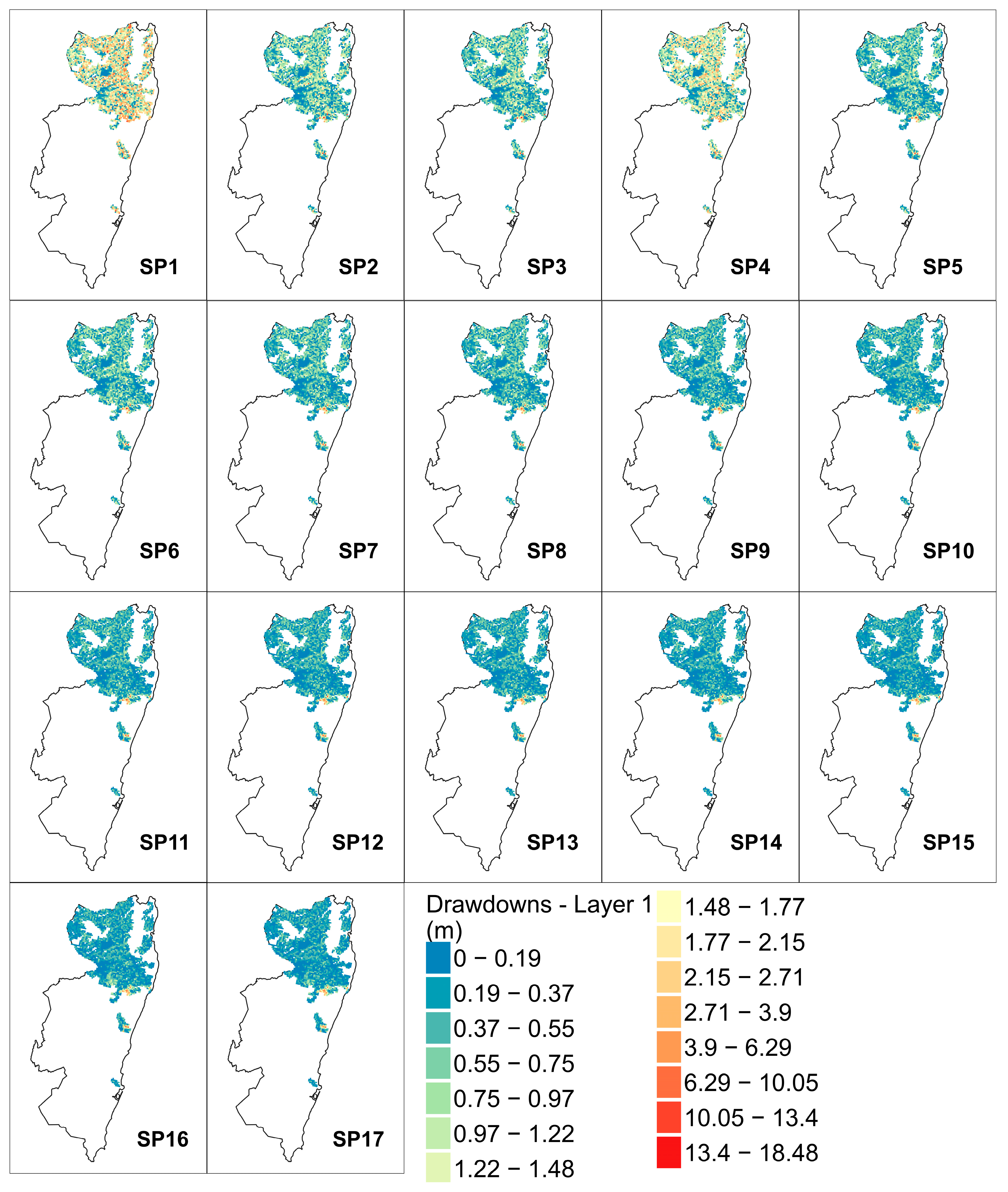
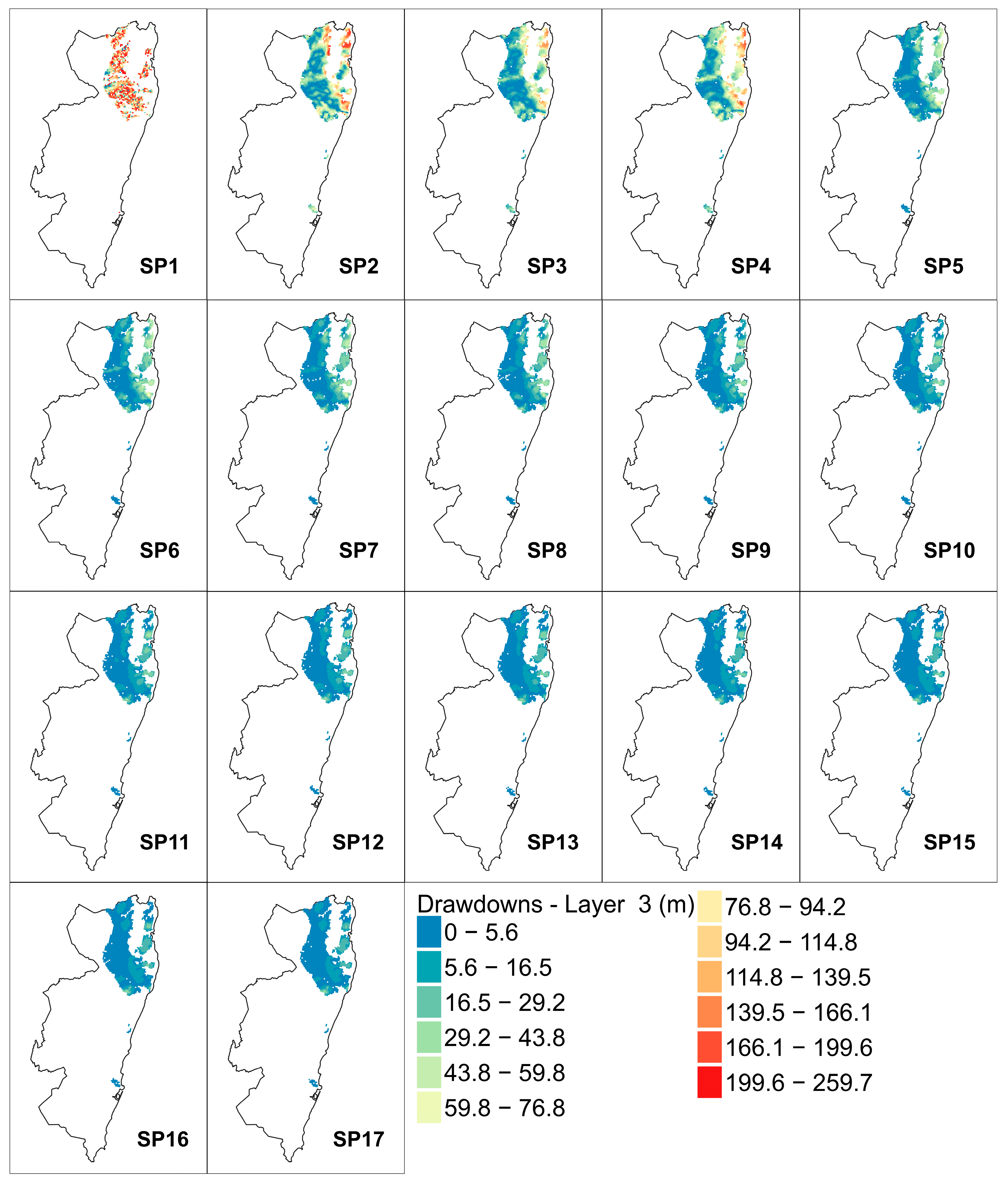
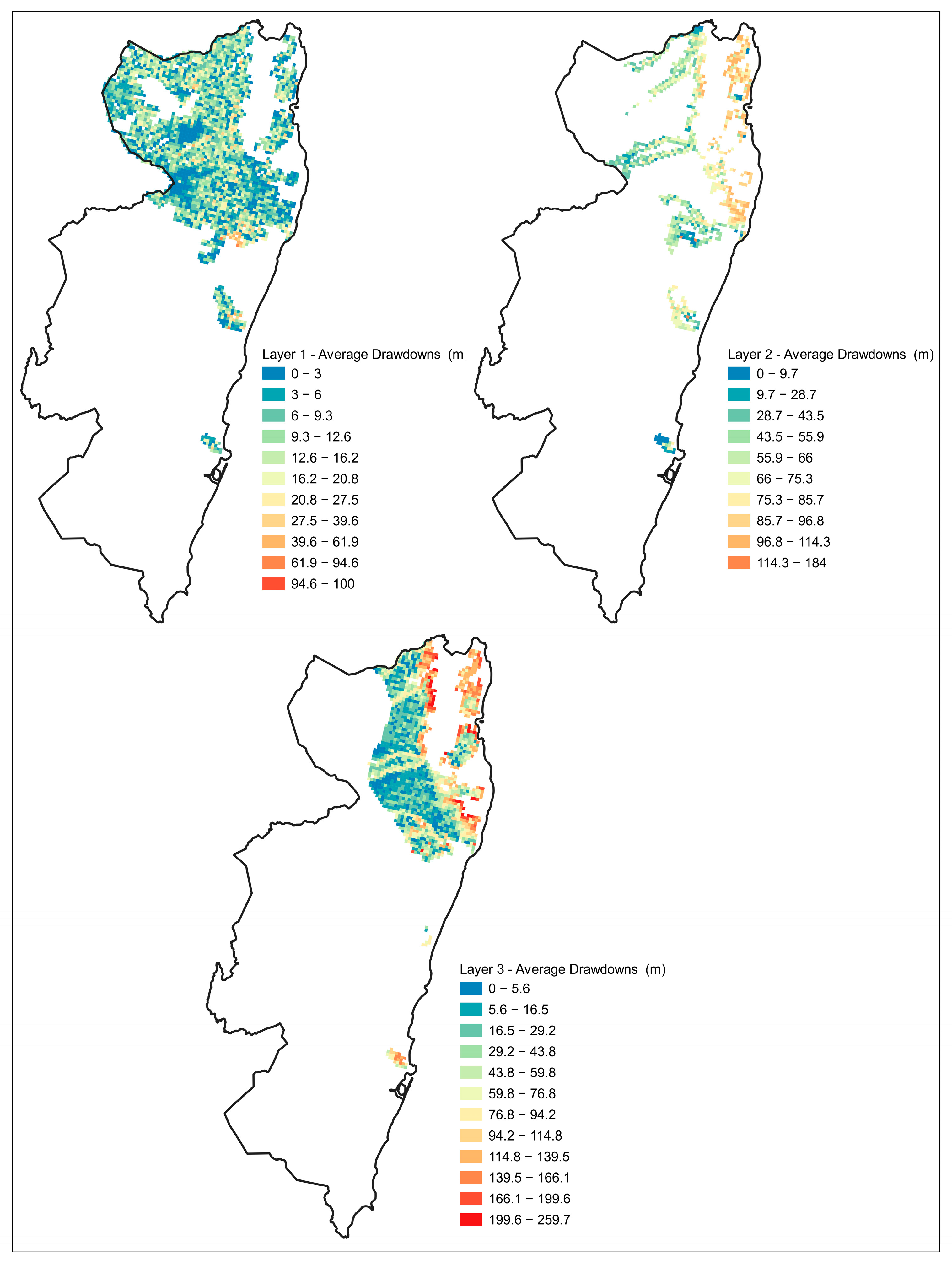
3.3. Drawdowns
4. Conclusions
Author Contributions
Funding
Data Availability Statement
Acknowledgments
Conflicts of Interest
References
- Stephens, G.L.; Slingo, J.M.; Rignot, E.; Reager, J.T.; Hakuba, M.Z.; Durack, P.J.; Worden, J.; Rocca, R. Earth’s Water Reservoirs in a Changing Climate. Proc. R. Soc. A. Math. Phys. Eng. Sci. 2020, 476, 20190458. [Google Scholar] [CrossRef] [PubMed]
- UNESCO. The United Nations World Water Development Report 2022: Groundwater: Making the Invisible Visible; Facts and Figures; United Nations Educational, Scientific and Cultural Organization: Paris, France, 2022; ISBN 9789231005077. [Google Scholar]
- Taylor, R.G.; Scanlon, B.; Döll, P.; Rodell, M.; Van Beek, R.; Wada, Y.; Longuevergne, L.; Leblanc, M.; Famiglietti, J.S.; Edmunds, M.; et al. Ground Water and Climate Change. Nat. Clim. Change 2013, 3, 322–329. [Google Scholar] [CrossRef]
- van der Gun, J. Groundwater and Global Change: Trends, Opportunities and Challenges. In The United Nations World Water Development Report-N 4; UNESCO: Paris, France, 2012; Volume 1, ISBN 9789230010492. [Google Scholar]
- de Graaf, I.E.; Gleeson, T.; Van Beek, L.P.H.; Sutanudjaja, E.H.; Bierkens, M.F. Environmental Flow Limits to Global Groundwater Pumping. Nature 2019, 574, 90–94. [Google Scholar] [CrossRef] [PubMed]
- Lawford, R.; Bogardi, J.; Marx, S.; Jain, S.; Wostl, C.P.; Knüppe, K.; Ringler, C.; Lansigan, F.; Meza, F. Basin Perspectives on the Water-Energy-Food Security Nexus. Curr. Opin. Environ. Sustain. 2013, 5, 607–616. [Google Scholar] [CrossRef]
- Postel, S.L. Entering an era of water scarcity: The challenges ahead. Ecol. Appl. 2000, 10, 941–948. [Google Scholar] [CrossRef]
- Wei, Y.; White, R.; Hu, K.; Willett, I. Valuing the Environmental Externalities of Oasis Farming in Left Banner, Alxa, China. Ecol. Econ. 2010, 69, 2151–2157. [Google Scholar] [CrossRef]
- Valdés-Pineda, R.; Pizarro, R.; García-Chevesich, P.; Valdés, J.B.; Olivares, C.; Vera, M.; Balocchi, F.; Pérez, F.; Vallejos, C.; Fuentes, R.; et al. Water Governance in Chile: Availability, Management and Climate Change. J. Hydrol. 2014, 519, 2538–2567. [Google Scholar] [CrossRef]
- Bauer, C.J. Water Conflicts and Entrenched Governance Problems in Chile’s Market Model. Water Altern. 2015, 8, 147–172. [Google Scholar]
- Carrera, J.; Hidalgo, J.J.; Slooten, L.J.; Vázquez-Suñé, E. Computational and Conceptual Issues in the Calibration of Seawaterintrusion Models. Hydrogeol. J. 2010, 18, 131–145. [Google Scholar] [CrossRef]
- Delsman, J.R.; Hu-A-Ng, K.R.M.; Vos, P.C.; De Louw, P.G.B.; Oude Essink, G.H.P.; Stuyfzand, P.J.; Bierkens, M.F.P. Paleo-Modeling of Coastal Saltwater Intrusion during the Holocene: An Application to the Netherlands. Hydrol. Earth Syst. Sci. 2014, 18, 3891–3905. [Google Scholar] [CrossRef]
- Nofal, E.R.; Amer, M.A.; El-Didy, S.M.; Fekry, A.M. Delineation and Modeling of Seawater Intrusion into the Nile Delta Aquifer: A New Perspective. Water Sci. 2015, 29, 156–166. [Google Scholar] [CrossRef]
- Meyer, R.; Engesgaard, P.; Sonnenborg, T.O. Origin and Dynamics of Saltwater Intrusion in a Regional Aquifer: Combining 3-D Saltwater Modeling with Geophysical and Geochemical Data. Water Resour. Res. 2019, 55, 1792–1813. [Google Scholar] [CrossRef]
- Chatton, E.; Aquilina, L.; Pételet-Giraud, E.; Cary, L.; Bertrand, G.; Labasque, T.; Hirata, R.; Martins, V.; Montenegro, S.; Vergnaud, V.; et al. Glacial Recharge, Salinisation and Anthropogenic Contamination in the Coastal Aquifers of Recife (Brazil). Sci. Total Environ. 2016, 569–570, 1114–1125. [Google Scholar] [CrossRef] [PubMed]
- IPCC. Special Report on the Ocean and Cryosphere in a Changing Climate; Cambridge University Press: Cambridge, UK; New York, NY, USA, 2019. [Google Scholar]
- Wassef, R.; Schüttrumpf, H. Impact of Sea-Level Rise on Groundwater Salinity at the Development Area Western Delta, Egypt. Groundw. Sustain. Dev. 2016, 2–3, 85–103. [Google Scholar] [CrossRef]
- Ehteshami, M.; Salari, M.; Zaresefat, M. Sustainable Development Analyses to Evaluate Groundwater Quality and Quantity Management. Model. Earth Syst. Environ. 2016, 2, 133. [Google Scholar] [CrossRef]
- Wang, G.Y.; You, G.; Shi, B.; Yu, J.; Tuck, M. Long-Term Land Subsidence and Strata Compression in Changzhou, China. Eng. Geol. 2009, 104, 109–118. [Google Scholar] [CrossRef]
- Dinh, N.; Nam, G.; Goto, A.; Osawa, K.; Nguyen, N.; Chau, V. Modeling for Analyzing Effects of Groundwater Pumping in Can Tho City, Vietnam. Int. Assoc. Lowl. Technol. 2019, 22, 33–43. [Google Scholar]
- Chrysanthopoulos, E.; Perdikaki, M.; Giannoulopoulos, P.; Kallioras, A. Groundwater Modeling of Coastal Aquifers Using Calibration in Pre-Development State. Environ. Earth Sci. 2024, 83, 382. [Google Scholar] [CrossRef]
- Reilly, T.E.; Harbaugh, A.W. Guidelines for Evaluating Ground-Water Flow Models; DIANE Publishing: Collingdale, PA, USA, 2004. [Google Scholar]
- Harbaugh, A.W. MODFLOW-2005, The US Geological Survey Modular Ground-Water Model: The Ground-Water Flow Process; US Department of the Interior, US Geological Survey: Reston, VA, USA, 2005. [Google Scholar]
- Anderson, M.P.; Woessner, W.W.; Hunt, R.J. Applied Groundwater Modeling: Simulation of Flow and Advective Transport, 2nd ed.; Academic Press: San Diego, CA, USA, 2015; ISBN 9780120581030. [Google Scholar]
- Ketemaw, T.; Hussien, A.; Woldemariyam Tesema, F.; Abadi Berhe, B. Numerical Groundwater Flow Modeling of Dijil River Catchment, Debre Markos Area, Ethiopia. Momona Ethiop. J. Sci. 2021, 13, 89–109. [Google Scholar] [CrossRef]
- Gropius, M.; Dahabiyeh, M.; Al Hyari, M.; Brückner, F.; Lindenmaier, F.; Vassolo, S. Estimation of Unrecorded Groundwater Abstractions in Jordan through Regional Groundwater Modelling. Hydrogeol. J. 2022, 30, 1769–1787. [Google Scholar] [CrossRef]
- Menichini, M.; Doveri, M. Modelling Tools for Quantitative Evaluations on the Versilia Coastal Aquifer System (Tuscany, Italy) in Terms of Groundwater Components and Possible Effects of Climate Extreme Events. Acque Sotter.-Ital. J. Groundw. 2020, 9, 35–44. [Google Scholar] [CrossRef]
- Rossetto, R.; De Filippis, G.; Borsi, I.; Foglia, L.; Cannata, M.; Criollo, R.; Vázquez-Suñé, E. Integrating Free and Open Source Tools and Distributed Modelling Codes in GIS Environment for Data-Based Groundwater Management. Environ. Model. Softw. 2018, 107, 210–230. [Google Scholar] [CrossRef]
- Bittner, D.; Rychlik, A.; Klöffel, T.; Leuteritz, A.; Disse, M.; Chiogna, G. A GIS-Based Model for Simulating the Hydrological Effects of Land Use Changes on Karst Systems–The Integration of the LuKARS Model into FREEWAT. Environ. Model. Softw. 2020, 127, 104682. [Google Scholar] [CrossRef]
- Bayanzul, B.; Nakamura, K.; Machida, I.; Watanabe, N.; Komai, T. Construction of a Conceptual Model for Confined Groundwater Flow in the Gunii Khooloi Basin, Southern Gobi Region, Mongolia. Hydrogeol. J. 2019, 27, 1581–1596. [Google Scholar] [CrossRef]
- Viguier, B.; Jourde, H.; Yáñez, G.; Lira, E.S.; Leonardi, V.; Moya, C.E.; García-Pérez, T.; Maringue, J.; Lictevout, E. Multidisciplinary Study for the Assessment of the Geometry, Boundaries and Preferential Recharge Zones of an Overexploited Aquifer in the Atacama Desert (Pampa del Tamarugal, Northern Chile). J. South Am. Earth Sci. 2018, 86, 366–383. [Google Scholar] [CrossRef]
- Francés, A.P.; Lubczynski, M.W.; Roy, J.; Santos, F.A.M.; Mahmoudzadeh Ardekani, M.R. Hydrogeophysics and Remote Sensing for the Design of Hydrogeological Conceptual Models in Hard Rocks–Sardón Catchment (Spain). J. Appl. Geophys. 2014, 110, 63–81. [Google Scholar] [CrossRef]
- Condon, L.E.; Kollet, S.; Bierkens, M.F.P.; Fogg, G.E.; Maxwell, R.M.; Hill, M.C.; Fransen, H.J.H.; Verhoef, A.; Van Loon, A.F.; Sulis, M.; et al. Global Groundwater Modeling and Monitoring: Opportunities and Challenges. Water Resour. Res. 2021, 57, e2020WR029500. [Google Scholar] [CrossRef]
- Severino, G.; Fallico, C.; Brunetti, G.F.A. Correlation Structure of Steady Well-Type Flows Through Heterogeneous Porous Media: Results and Application. Water Resour. Res. 2024, 60, e2023WR036279. [Google Scholar] [CrossRef]
- IPCC. Climate Change 2022: Impacts, Adaptation and Vulnerability: Contribution of Working Group II to the Sixth Assessment Report of the Intergovernmental Panel on Climate Change; Cambridge University Press: Cambridge, UK, 2022. [Google Scholar]
- Doherty, J.; Simmons, C.T. Groundwater Modelling in Decision Support: Reflections on a Unifiedconceptual Framework. Hydrogeol. J. 2013, 21, 1531–1537. [Google Scholar] [CrossRef]
- Liang, E.; Wang, J. Advanced Remote Sensing: Terrestrial Information Extraction and Applications; Academic Press: Cambridge, MA, USA; Informa UK Ltd.: London, UK, 2019; Volume 2, p. 992. [Google Scholar]
- Nobre, B.V.B.; Cirilo, J.A. Hydrological Modeling Applied to Water Synergy Evaluation in Castanhão Reservoir, Ceará, Brazil. Environ. Monit. Assess. 2025, 197, 115. [Google Scholar] [CrossRef]
- de Arruda Gomes, M.M.; de Melo Verçosa, L.F.; Cirilo, J.A. Hydrologic Models Coupled with 2D Hydrodynamic Model for High-Resolution Urban Flood Simulation. Nat. Hazards 2021, 108, 3121–3157. [Google Scholar] [CrossRef]
- Cirilo, J.A.; Verçosa, L.F.d.M.; Gomes, M.M.d.A.; Feitoza, M.A.B.; Ferraz, G.d.F.; Silva, B.d.M. Development and Application of a Rainfall-Runoff Model for Semi-Arid Regions. Braz. J. Water Resour. 2020, 25, e15. [Google Scholar] [CrossRef]
- Virães, M.V.; Cirilo, J.A. Regionalization of Hydrological Model Parameters for the Semi-Arid Region of the Northeast Brazil. Rev. Bras. Recur. Hidr. 2019, 24, e49. [Google Scholar] [CrossRef]
- de Oliveira, G.A.; da Silva Ribeiro, A.A.; Cirilo, J.A. Collaborative Spatial Information as an Alternative Data Source for Hydrodynamic Model Calibration: A Pernambuco State Case Study, Brazil. Nat. Hazards 2023, 118, 1535–1559. [Google Scholar] [CrossRef]
- Souza, J.D.S.d.; Cirilo, J.A.; Bezerra, S.d.T.M.; Oliveira, G.A.d.; Freire, G.D.; Coutinho, A.P.; Cabral, J.J.d.S.P. Decision Support System for the Integrated Management of Multiple Supply Systems in the Brazilian Semiarid Region. Water 2023, 15, 223. [Google Scholar] [CrossRef]
- Silva, M.C.d.O.; Vasconcelos, R.S.; Cirilo, J.A. Risk Mapping of Water Supply and Sanitary Sewage Systems in a City in the Brazilian Semi-Arid Region Using GIS-MCDA. Water 2022, 14, 3251. [Google Scholar] [CrossRef]
- Cirilo, J.A.; Ribeiro Neto, A.; Ramos, N.M.R.; Fortunato, C.F.; de Souza, J.D.S.; Bezerra, S.d.T.M. Management of Water Supply Systems from Interbasin Transfers: Case Study in the Brazilian Semiarid Region. Urban Water J. 2021, 18, 660–671. [Google Scholar] [CrossRef]
- Do Amaral, F.E.; Cirilo, J.A.; Neto, A.R. Use of Geoprocessing Techniques in the Optimization of the Pipeline Alignment of Water Supply Systems with the Use of a High Definition Database. Eng. Sanit. E. Ambient. 2020, 25, 381–391. [Google Scholar] [CrossRef]
- Ribeiro, A.A.d.S.; de Oliveira, G.A.; Cirilo, J.A.; Alves, F.H.B.; Batista, L.F.D.R.; Melo, V.B. Floodplain Reconstitution Based on Data Collected via Smartphones: A Methodological Approach to Hydrological Risk Mapping. Rev. Bras. Recur. Hidr. 2020, 25, e41. [Google Scholar] [CrossRef]
- Lima Neto, O.C.; Ribeiro Neto, A.; Alves, F.H.B.; Cirilo, J.A. Sub-Daily Hydrological-Hydrodynamic Simulation in Flash Flood Basins: Una River (Pernambuco/Brazil). Rev. Ambiente E. Agua 2020, 15, e2256. [Google Scholar] [CrossRef]
- Lins, R.C.; Martinez, J.M.; Marques, D.d.M.; Cirilo, J.A.; Medeiros, P.R.P.; Júnior, C.R.F. A Multivariate Analysis Framework to Detect Key Environmental Factors Affecting Spatiotemporal Variability of Chlorophyll-a in a Tropical Productive Estuarine-Lagoon System. Remote Sens 2018, 10, 853. [Google Scholar] [CrossRef]
- Adhikari, R.K.; Yilmaz, A.G.; Mainali, B.; Dyson, P.; Imteaz, M.A. Methods of Groundwater Recharge Estimation under Climate Change: A Review. Sustainability 2022, 14, 15619. [Google Scholar] [CrossRef]
- Kumar, P.J.S.; Schneider, M.; Elango, L. The State-of-the-Art Estimation of Groundwater Recharge and Water Balance with a Special Emphasis on India: A Critical Review. Sustainability 2022, 14, 340. [Google Scholar] [CrossRef]
- Martos-Rosillo, S.; González-Ramón, A.; Jiménez-Gavilán, P.; Andreo, B.; Durán, J.J.; Mancera, E. Review on Groundwater Recharge in Carbonate Aquifers from SW Mediterranean (Betic Cordillera, S Spain). Environ. Earth Sci. 2015, 74, 7571–7581. [Google Scholar] [CrossRef]
- Coelho, V.H.R.; Montenegro, S.; Almeida, C.N.; Silva, B.B.; Oliveira, L.M.; Gusmão, A.C.V.; Freitas, E.S.; Montenegro, A.A.A. Alluvial Groundwater Recharge Estimation in Semi-Arid Environment Using Remotely Sensed Data. J. Hydrol. 2017, 548, 1–15. [Google Scholar] [CrossRef]
- Yang, X.; Dai, C.; Liu, G.; Li, C. Research on the Jiamusi Area’s Shallow Groundwater Recharge Using Remote Sensing and the SWAT Model. Appl. Sci. 2024, 14, 7220. [Google Scholar] [CrossRef]
- Szilagyi, J.; Jozsa, J. MODIS-Aided Statewide Net Groundwater-Recharge Estimation in Nebraska. Groundwater 2013, 51, 735–744. [Google Scholar] [CrossRef]
- Silva, C.d.O.F.; Manzione, R.L.; Albuquerque Filho, J.L. Combining Remotely Sensed Actual Evapotranspiration and GIS Analysis for Groundwater Level Modeling. Environ. Earth Sci. 2019, 78, 462. [Google Scholar] [CrossRef]
- Barbosa, L.R.; Coelho, V.H.R.; Gusmão, A.C.V.L.; Fernandes, L.A.; da Silva, B.B.; Galvão, C.d.O.; Caicedo, N.O.L.; da Paz, A.R.; Xuan, Y.; Bertrand, G.F.; et al. A Satellite-Based Approach to Estimating Spatially Distributed Groundwater Recharge Rates in a Tropical Wet Sedimentary Region despite Cloudy Conditions. J. Hydrol. 2022, 607, 127503. [Google Scholar] [CrossRef]
- Fallatah, O.A.; Ahmed, M.; Cardace, D.; Boving, T.; Akanda, A.S. Assessment of Modern Recharge to Arid Region Aquifers Using an Integrated Geophysical, Geochemical, and Remote Sensing Approach. J. Hydrol. 2019, 569, 600–611. [Google Scholar] [CrossRef]
- Gemitzi, A.; Ajami, H.; Richnow, H.H. Developing Empirical Monthly Groundwater Recharge Equations Based on Modeling and Remote Sensing Data–Modeling Future Groundwater Recharge to Predict Potential Climate Change Impacts. J. Hydrol. 2017, 546, 1–13. [Google Scholar] [CrossRef]
- Githui, F.; Selle, B.; Thayalakumaran, T. Recharge Estimation Using Remotely Sensed Evapotranspiration in an Irrigated Catchment in Southeast Australia. Hydrol. Process. 2012, 26, 1379–1389. [Google Scholar] [CrossRef]
- Knoche, M.; Fischer, C.; Pohl, E.; Krause, P.; Merz, R. Combined Uncertainty of Hydrological Model Complexity and Satellite-Based Forcing Data Evaluated in Two Data-Scarce Semi-Arid Catchments in Ethiopia. J. Hydrol. 2014, 519, 2049–2066. [Google Scholar] [CrossRef]
- González-Ortigoza, S.; Hernández-Espriú, A.; Arciniega-Esparza, S. Regional Modeling of Groundwater Recharge in the Basin of Mexico: New Insights from Satellite Observations and Global Data Sources. Hydrogeol. J. 2023, 31, 1971–1990. [Google Scholar] [CrossRef]
- El-Hadidy, S.M.; Morsy, S.M. Expected Spatio-Temporal Variation of Groundwater Deficit by Integrating Groundwater Modeling, Remote Sensing, and GIS Techniques. Egypt. J. Remote Sens. Space Sci. 2022, 25, 97–111. [Google Scholar] [CrossRef]
- Belay, A.S.; Yenehun, A.; Nigate, F.; Tilahun, S.A.; Dessie, M.; Moges, M.M.; Chen, M.; Fentie, D.; Adgo, E.; Nyssen, J.; et al. Estimation of Spatially Distributed Groundwater Recharge in Data-Scarce Regions. J. Hydrol. Reg. Stud. 2024, 56, 102072. [Google Scholar] [CrossRef]
- Santarosa, L.V.; Pinto, G.V.F.; Blandón Luengas, J.S.; Gastmans, D. Remote Sensing to Quantify Potential Aquifer Recharge as a Complementary Tool for Groundwater Monitoring. Hydrol. Sci. J. 2024. [Google Scholar] [CrossRef]
- Castellazzi, P.; Longuevergne, L.; Martel, R.; Rivera, A.; Brouard, C.; Chaussard, E. Quantitative Mapping of Groundwater Depletion at the Water Management Using a Combined GRACE/InSAR Approach. Remote Sens. Environ. 2018, 205, 408–418. [Google Scholar] [CrossRef]
- Ouyang, L.; Zhao, Z.; Zhou, D.; Cao, J.; Qin, J.; Cao, Y.; He, Y. Study on the Relationship between Groundwater and Land Subsidence in Bangladesh Combining GRACE and InSAR. Remote Sens. 2024, 16, 3715. [Google Scholar] [CrossRef]
- Brunetti, G.F.A.; Maiolo, M.; Fallico, C.; Severino, G. Unraveling the Complexities of a Highly Heterogeneous Aquifer under Convergent Radial Flow Conditions. Eng. Comput. 2024, 40, 3115–3130. [Google Scholar] [CrossRef]
- Koltsida, E.; Kallioras, A. Groundwater Flow Simulation through the Application of the FREEWAT Modeling Platform. J. Hydroinformatics 2019, 21, 812–833. [Google Scholar] [CrossRef]
- De Filippis, G.; Ghetta, M.; Neumann, J.; Cardoso, M.; Cannata, M.; Borsi, I.; Rossetto, R. Groundwater Modeling Using MODFLOW-OWHM (One Water Hydrologic Flow Model). In FREEWAT User Manual; 2017; Volume 1, Available online: http://www.freewat.eu/sites/default/files/FREEWAT_vol1.pdf (accessed on 13 April 2025).
- De Filippis, G.; Pouliaris, C.; Kahuda, D.; Vasile, T.A.; Manea, V.A.; Zaun, F.; Panteleit, B.; Dadaser-Celik, F.; Positano, P.; Nannucci, M.S.; et al. Spatial Data Management and Numerical Modelling: Demonstrating the Application of the QGIS-Integrated FREEWAT Platform at 13 Case Studies for Tackling Groundwater Resource Management. Water 2020, 12, 41. [Google Scholar] [CrossRef]
- Associação Pernambuca de Águas e Clima (APAC). A Gestão das Águas Subterrâneas em Pernambuco; Associação Pernambuca de Águas e Clima (APAC): Recife, Brazil, 2021. [Google Scholar]
- Cabral, J.J.; Santos, S.M.; Montenegro, S.M.; Demetrio, J.G.; Cirilo, J.A.; Manoel Filho, J.; Santos, A.C.; Montenegro, A.A. Ferramentas para o gerenciamento integrado dos aqüíferos da Região Metropolitana de Recife. In Proceedings of the XIII Simpósio Brasileiro de Recursos Hídricos, Belo Horizonte, Brazil, 28 November–2 December 1999; pp. 1–11. [Google Scholar]
- de Luna, R.M.R.; Garnés, S.J.d.A.; Cabral, J.J.d.S.P.; dos Santos, S.M. Groundwater Overexploitation and Soil Subsidence Monitoring on Recife Plain (Brazil). Nat. Hazards 2017, 86, 1363–1376. [Google Scholar] [CrossRef]
- Louwyck, A.; Vandenbohede, A.; Heuvelmans, G.; Van Camp, M.; Walraevens, K. The Water Budget Myth and Its Recharge Controversy: Linear vs. Nonlinear Models. Groundwater 2023, 61, 100–110. [Google Scholar] [CrossRef]
- IBGE. Instituto Brasileiro de Geografia e Estatística Censo Demográfico 2022: Resultados Preliminares da Amostra. 2022. Available online: https://www.ibge.gov.br/estatisticas/sociais/saude/22827-censo-demografico-2022.html (accessed on 13 April 2025).
- Coelho, V.H.R.; Bertrand, G.F.; Montenegro, S.M.G.L.; Paiva, A.L.R.; Almeida, C.N.; Galvão, C.O.; Barbosa, L.R.; Batista, L.F.D.R.; Ferreira, E.L.G.A. Piezometric Level and Electrical Conductivity Spatiotemporal Monitoring as an Instrument to Design Further Managed Aquifer Recharge Strategies in a Complex Estuarial System under Anthropogenic Pressure. J. Environ. Manag. 2018, 209, 426–439. [Google Scholar] [CrossRef] [PubMed]
- Cary, L.; Petelet-Giraud, E.; Bertrand, G.; Kloppmann, W.; Aquilina, L.; Martins, V.; Hirata, R.; Montenegro, S.; Pauwels, H.; Chatton, E.; et al. Origins and Processes of Groundwater Salinization in the Urban Coastal Aquifers of Recife (Pernambuco, Brazil): A Multi-Isotope Approach. Sci. Total Environ. 2015, 530–531, 411–429. [Google Scholar] [CrossRef]
- Lopes, A.V.G. Aspectos Hidrogeológicos Ambientais e Jurídicos Como Ferramenta para Uso e Proteção das Águas Subterrâneas da Região Metropolitana do Recife; Universidade Federal de Pernambuco: Recife, Brazil, 2012. [Google Scholar]
- Leitão, T.; Costa, W.D.; Oliveira, M.M.; Novo, M.E.; Martins, T.; Henriques, M.J.; Charneca, N.; Lobo Ferreira, J.P.; Viseu, M.T.; Santos, M.A.V.; et al. Estudos Sobre a Disponibilidade e Vulnerabilidade dos Recursos Hídricos Subterrâneos da Região Metropolitana do Recife; Silusba: Recife, Brazil, 2017. [Google Scholar]
- Pfaltzgraff, P.A.S.; Leal, O.; Souza Júnior, L.C.; Lins, C.A.C.; Souza, F.J.C.; Accioly, A.C.A.; Santos, A.S.; Melo, C.R.; Moreira, F.M.; Almeida, I.S.; et al. Sistema de Informações Geoambientais da Região Metropolitana do Recife; RIGeo: Recife, Brazil, 2003. [Google Scholar]
- Costa, W.D.; Filho, J.M.; Santos, A.C.; Costa Filho, W.D.; Monteiro, A.B.; Souza, F.J.A. De Zoneamento de Explotação das Águas Subterrâneas na Cidade do. X Congr. Bras. Águas Subterrâneas 1998, 1–11. [Google Scholar]
- Costa, W.D.; Santos, A.C.; Costa Filho, W.D. O controle estrutural na formação dos aquíferos na planície do Recife. In Proceedings of the UFPE-Universidade Federal de Pernambuco, Anais do 8. Congresso Brasileiro de Águas Subterrâneas, ABAS, Recife, Brazil, 2 October 1994. [Google Scholar]
- McDonald, M.G.; Harbaugh, A.W. A Modular Three-Dimensional Finite-Difference Ground-Water Flow Model; Geological Survey: Reston, VA, USA, 1988. [Google Scholar]
- Rossetto, R.; Borsi, I.; Foglia, L. FREEWAT: FREE and Open Source Software Tools for WATer Resource Management. Rend. Online della Soc. Geol. Ital. 2015, 35, 252–255. [Google Scholar] [CrossRef]
- Monteiro, A.B. Modelagem do Fluxo Subterrâneo Nos Aqüíferos da Planície do Recife e Seus Encaixes. Master’s Thesis, Universidade Federal de Pernambuco, Recife, Brazil, 2000. [Google Scholar]
- Diniz, J.A.O.; Monteiro, A.B.; Silva, R.C.; Paula, T.L.F. Mapa Hidrogeológico Do Brasil AO Milionésimo: Nota Técnica; CPRM: Recife, Brazil, 2014. [Google Scholar]
- Lobo Ferreira, J.P. Mathematical Model for the Evaluation of the Recharge of Aquifers in Semiarid Regions with Scarce (Lack) Hydrogeological Data. Eur. Mech. Colloq. Euromech 1981, 143. [Google Scholar]
- Barbosa, S.A.; Jones, N.L.; Williams, G.P.; Mamane, B.; Begou, J.; Nelson, E.J.; Ames, D.P. Exploiting Earth Observations to Enable Groundwater Modeling in the Data-Sparse Region of Goulbi Maradi, Niger. Remote Sens. 2023, 15, 5199. [Google Scholar] [CrossRef]
- Embrapa-Empresa Brasileira de Agropecuária. Zoneamento Agroecológico do Estado de Pernambuco. 2001. Available online: https://www.embrapa.br/busca-de-solucoes-tecnologicas/-/produto-servico/4697/zoneamento-agroecologico-do-estado-de-pernambuco-zape (accessed on 13 April 2025).
- ASTM Designation: D 5611-94 e1; Standard Guide for Conducting a Sensitivity Analysis for a Ground-Water Flow Model Application. ASTM: West Conshohocken, PA, USA, 2021.
- Ye, M.; Pohlmann, K.F.; Chapman, J.B.; Pohll, G.M.; Reeves, D.M. A Model-Averaging Method for Assessing Groundwater Conceptual Model Uncertainty. Ground Water 2010, 48, 716–728. [Google Scholar] [CrossRef] [PubMed]
- Ahmadi, A.; Olyaei, M.; Heydari, Z.; Emami, M.; Zeynolabedin, A.; Ghomlaghi, A.; Daccache, A.; Fogg, G.E.; Sadegh, M. Groundwater Level Modeling with Machine Learning: A Systematic Review and Meta-Analysis. Water 2022, 14, 949. [Google Scholar] [CrossRef]
- Rafik, A.; Ait Brahim, Y.; Amazirh, A.; Ouarani, M.; Bargam, B.; Ouatiki, H.; Bouslihim, Y.; Bouchaou, L.; Chehbouni, A. Groundwater Level Forecasting in a Data-Scarce Region through Remote Sensing Data Downscaling, Hydrological Modeling, and Machine Learning: A Case Study from Morocco. J. Hydrol. Reg. Stud. 2023, 50, 101569. [Google Scholar] [CrossRef]
- Malekzadeh, M.; Kardar, S.; Shabanlou, S. Simulation of Groundwater Level Using MODFLOW, Extreme Learning Machine and Wavelet-Extreme Learning Machine Models. Groundw. Sustain. Dev. 2019, 9, 100279. [Google Scholar] [CrossRef]
- Teimoori, S.; Olya, M.H.; Miller, C.J. Groundwater Level Monitoring Network Design with Machine Learning Methods. J. Hydrol. 2023, 625, 130145. [Google Scholar] [CrossRef]
- Elmotawakkil, A.; Sadiki, A.; Enneya, N. Predicting Groundwater Level Based on Remote Sensing and Machine Learning: A Case Study in the Rabat-Kénitra Region. J. Hydroinform. 2024, 26, 2639–2667. [Google Scholar] [CrossRef]
- Evans, S.; Williams, G.P.; Jones, N.L.; Ames, D.P.; Nelson, E.J. Exploiting Earth Observation Data to Impute Groundwater Level Measurements with an Extreme Learning Machine. Remote Sens. 2020, 12, 2044. [Google Scholar] [CrossRef]
- Costa, W.D.; Monteiro, A.B.; Costa Filho, W.D.; Santos, A.C. Condicionamento Hidrogeológico da Explotação do Aqüífero Costeiro Boa Viagem; Congresso Mundial Integrado de Águas Subterrâneas: Fortaleza, Brazil, 2000. [Google Scholar]
- Costa, W.D.; Costa, H.F.; Ferreira, C.A.; Morais, J.F.S.d.; Villa Verde, E.R.; Costa, L.B. Estudo Hidrogeológico dos Municípios de Recife, Olinda, Camaragibe e Jaboatão dos Guararapes-Hidrorec II; Revista Águas Subterrâneas: Recife, Brazil, 2002. [Google Scholar]
- Duarte Costa, W.; Duarte, W.; Filho, C. A gestão dos aqüíferos costeiros de Pernambuco. In Proceedings of the Anais do XIII Congresso Brasileiro de Águas Subterrâneas. Águas Subterrâneas, Recife, Brazil, 20 September 2004; pp. 1–13. [Google Scholar]
- Cao, G.; Zheng, C.; Scanlon, B.R.; Liu, J.; Li, W. Use of Flow Modeling to Assess Sustainability of Groundwater Resources in the North China Plain. Water Resour. Res. 2013, 49, 159–175. [Google Scholar] [CrossRef]
- Haq, F.u.; Naeem, U.A.; Gabriel, H.F.; Khan, N.M.; Ahmad, I.; Ur Rehman, H.; Zafar, M.A. Impact of Urbanization on Groundwater Levels in Rawalpindi City, Pakistan. Pure Appl. Geophys. 2021, 178, 491–500. [Google Scholar] [CrossRef]
- Jayakumar, R.; Lee, E. Climate Change and Groundwater Conditions in the Mekong Region-A Review. J. Groundw. Sci. Eng. 2017, 5, 14–30. [Google Scholar] [CrossRef]
- Fan, X.; Peterson, T.J.; Henley, B.J.; Arora, M. Groundwater Sensitivity to Climate Variations Across Australia. Water Resour. Res. 2023, 59, e2023WR035036. [Google Scholar] [CrossRef]
- Gunduz, O.; Simsek, C. Influence of Climate Change on Shallow Groundwater Resources: The Link between Precipitation and Groundwater Levels in Alluvial Systems. NATO Sci. Peace Secur. Ser. C Environ. Secur. 2011, 3, 225–233. [Google Scholar] [CrossRef]
- Borba, A.L.S.; Costa Filho, W.D.; Mascarenhas, J.C. Configuração geométrica dos aquíferos da Região Metropolitana do Recife. In Proceedings of the XVI Congresso Brasileiro de Águas Subterrâneas e XVII Encontro Nacional de Perfuradores de Poços, Recife, Brazil, 6 September 2010. [Google Scholar]
- Makhlouf, A.; El-Rawy, M.; Kanae, S.; Ibrahim, M.G.; Sharaan, M. Integrating MODFLOW and Machine Learning for Detecting Optimum Groundwater Abstraction Considering Sustainable Drawdown and Climate Changes. J. Hydrol. 2024, 637, 131428. [Google Scholar] [CrossRef]
- Majumdar, S.; Smith, R.; Butler, J.J.; Lakshmi, V. Groundwater Withdrawal Prediction Using Integrated Multitemporal Remote Sensing Data Sets and Machine Learning. Water Resour. Res. 2020, 56, e2020WR028059. [Google Scholar] [CrossRef]
- Majumdar, S.; Smith, R.; Conway, B.D.; Lakshmi, V. Advancing Remote Sensing and Machine Learning-Driven Frameworks for Groundwater Withdrawal Estimation in Arizona: Linking Land Subsidence to Groundwater Withdrawals. In Proceedings of the Hydrological Processes; John Wiley and Sons Ltd.: Hoboken, NJ, USA, 2022. [Google Scholar]
- Li, J.; Li, F.; Li, H.; Guo, C.; Dong, W. Analysis of Rainfall Infiltration and Its Influence on Groundwater in Rain Gardens. Environ. Sci. Pollut. Res. 2019, 26, 22641–22655. [Google Scholar] [CrossRef]
- Moretti, L.; Altobelli, L.; Cantisani, G.; Del Serrone, G. Permeable Interlocking Concrete Pavements: A Sustainable Solution for Urban and Industrial Water Management. Water 2025, 17, 829. [Google Scholar] [CrossRef]


| Stress Period (SP) | Length (Days) | Date | Recharge |
|---|---|---|---|
| 1 | 731 | 1 January 2004–31 December 2005 | Daily Average from 2004 to 2005 |
| 2 | 365 | 1 January–31 December 2006 | Daily Average from 2006 |
| 3 | 365 | 1 January–31 December 2007 | Daily Average from 2007 |
| 4 | 731 | 1 January 2008–31 December 2009 | Daily Average from 2008 to 2009 |
| 5 | 365 | 1 January–31 December 2010 | Daily Average from 2010 |
| 6 | 365 | 1 January–31 December 2011 | Daily Average from 2011 |
| 7 | 366 | 1 January–31 December 2012 | Daily Average from 2012 |
| 8 | 730 | 1 January 2013–31 December 2014 | Daily Average from 2013 to 2014 |
| 9 | 365 | 1 January–31 December 2015 | Daily Average from 2015 |
| 10 | 366 | 1 January–31 December 2016 | Daily Average from 2016 |
| 11 | 365 | 1 January–31 December 2017 | Daily Average from 2017 |
| 12 | 365 | 1 January–31 December 2018 | Daily Average from 2018 |
| 13 | 365 | 1 January–31 December 2019 | Daily Average from 2019 |
| 14 | 366 | 1 January–31 December 2020 | Daily Average from 2020 |
| 15 | 365 | 1 January–31 December 2021 | Daily Average from 2021 |
| 16 | 365 | 1 January–31 December 2022 | Daily Average from 2022 |
| 17 | 365 | 1 January–31 December 2023 | Daily Average from 2023 |
| Parameter | Value |
|---|---|
| R2 | 0.97 |
| r | 0.98 |
| RRMSE | 23.96 |
| MARE | 42.96 |
| Formations | Barreiras | Algodoais | Beberibe | Cabo | Alluvial Deposits | Coastal Deposit | Estiva | |
|---|---|---|---|---|---|---|---|---|
| Input | Storage | 1346.23 | 0.16 | 181.09 | 0.84 | 387.13 | 187.02 | 0.01 |
| Constant potential | 1.74 | 0.00 | 0.02 | 0.00 | 0.15 | 6.84 | 0.00 | |
| Well | 0.00 | 0.00 | 0.00 | 0.00 | 0.00 | 0.00 | 0.00 | |
| Drain | 0.00 | 0.00 | 0.00 | 0.00 | 0.00 | 0.00 | 0.00 | |
| Recharge | 174.40 | 8.38 | 142.73 | 0.38 | 592.24 | 1050.09 | 0.26 | |
| Sea | 0.00 | 0.00 | 0.00 | 0.00 | 4.81 | 3.20 | 0.00 | |
| Barreiras | 0.00 | 0.04 | 51.41 | 0.00 | 355.69 | 140.92 | 0.00 | |
| Algodoais | 0.00 | 0.00 | 0.00 | 0.00 | 0.12 | 0.10 | 0.00 | |
| Beberibe | 4.17 | 0.00 | 0.00 | 0.00 | 59.26 | 0.86 | 0.00 | |
| Cabo | 0.00 | 0.03 | 0.00 | 0.00 | 6.97 | 7.46 | 0.00 | |
| Alluvial Deposits | 8.37 | 0.03 | 153.05 | 20.89 | 0.00 | 17.53 | 0.00 | |
| Coastal Deposit | 0.66 | 0.03 | 173.05 | 11.62 | 23.00 | 0.00 | 0.00 | |
| Estiva | 0.00 | 0.00 | 0.00 | 0.00 | 0.00 | 0.02 | 0.00 | |
| Gramame | 0.31 | 0.00 | 34.46 | 0.00 | 0.49 | 4.28 | 0.00 | |
| Maria Farinha | 0.00 | 0.00 | 1.09 | 0.00 | 0.00 | 0.13 | 0.00 | |
| Mangrove Sediments | 0.00 | 0.01 | 0.05 | 0.02 | 0.10 | 0.10 | 0.00 | |
| Ipojuca Suite | 0.00 | 0.00 | 0.00 | 0.01 | 0.08 | 0.04 | 0.00 | |
| Total | 1535.88 | 8.67 | 736.96 | 33.75 | 1430.04 | 1418.60 | 0.28 | |
| Output | Storage | 631.87 | 8.28 | 440.01 | 2.43 | 1055.02 | 940.55 | 0.26 |
| Constant potential | 6.50 | 0.00 | 0.00 | 0.00 | 4.81 | 4.03 | 0.00 | |
| Well | 116.32 | 0.00 | 214.13 | 16.85 | 110.21 | 217.74 | 0.00 | |
| Drain | 179.72 | 0.15 | 17.56 | 0.00 | 63.36 | 31.53 | 0.00 | |
| Recharge | 0.00 | 0.00 | 0.00 | 0.00 | 0.00 | 0.00 | 0.00 | |
| Sea | 1.26 | 0.00 | 0.00 | 0.00 | 0.15 | 6.66 | 0.00 | |
| Barreiras | 0.00 | 0.00 | 4.17 | 0.00 | 8.37 | 0.66 | 0.00 | |
| Algodoais | 0.04 | 0.00 | 0.00 | 0.03 | 0.03 | 0.03 | 0.00 | |
| Beberibe | 51.41 | 0.00 | 0.00 | 0.00 | 153.05 | 173.05 | 0.00 | |
| Cabo | 0.00 | 0.00 | 0.00 | 0.00 | 20.89 | 11.62 | 0.00 | |
| Alluvial Deposits | 355.69 | 0.12 | 59.26 | 6.97 | 0.00 | 23.00 | 0.00 | |
| Coastal Deposit | 140.92 | 0.10 | 0.86 | 7.46 | 17.53 | 0.00 | 0.02 | |
| Estiva | 0.00 | 0.00 | 0.00 | 0.00 | 0.00 | 0.00 | 0.00 | |
| Gramame | 47.60 | 0.00 | 0.54 | 0.00 | 1.01 | 6.13 | 0.00 | |
| Maria Farinha | 1.00 | 0.00 | 0.00 | 0.00 | 0.00 | 0.65 | 0.00 | |
| Mangrove Sediments | 0.15 | 0.01 | 0.40 | 0.01 | 0.02 | 0.06 | 0.00 | |
| Ipojuca Suite | 0.00 | 0.00 | 0.00 | 0.00 | 0.01 | 0.01 | 0.00 | |
| Total | 1532.47 | 8.67 | 736.95 | 33.75 | 1434.46 | 1415.73 | 0.28 | |
| In–Out | 3.41 | 0.01 | 0.01 | 0.00 | −4.42 | 2.87 | 0.00 | |
| Percentage of discrepancy | 0.00 | 0.00 | 0.00 | 0.00 | 0.00 | 0.00 | 0.00 | |
| Formations | Gramame | Maria Farinha | Mangrove Sediments | Ipojuca Suite | ||||
| Input | Storage | 9.36 | 0.50 | 1.78 | 0.15 | |||
| Constant potential | 0.00 | 0.00 | 0.00 | 0.00 | ||||
| Well | 0.00 | 0.00 | 0.00 | 0.00 | ||||
| Drain | 0.00 | 0.00 | 0.00 | 0.00 | ||||
| Recharge | 12.10 | 0.18 | 83.53 | 0.32 | ||||
| Sea | 0.00 | 0.00 | 0.00 | 0.00 | ||||
| Barreiras | 47.60 | 1.00 | 0.15 | 0.00 | ||||
| Algodoais | 0.00 | 0.00 | 0.01 | 0.00 | ||||
| Beberibe | 0.54 | 0.00 | 0.40 | 0.00 | ||||
| Cabo | 0.00 | 0.00 | 0.01 | 0.00 | ||||
| Alluvial Deposits | 1.01 | 0.00 | 0.02 | 0.01 | ||||
| Coastal Deposit | 6.13 | 0.65 | 0.06 | 0.01 | ||||
| Estiva | 0.00 | 0.00 | 0.00 | 0.00 | ||||
| Gramame | 0.00 | 0.21 | 0.07 | 0.00 | ||||
| Maria Farinha | 0.13 | 0.00 | 0.00 | 0.00 | ||||
| Mangrove Sediments | 0.02 | 0.01 | 0.00 | 0.00 | ||||
| Ipojuca Suite | 0.00 | 0.00 | 0.00 | 0.00 | ||||
| Total | 76.89 | 2.55 | 86.02 | 0.49 | ||||
| Output | Storage | 36.19 | 1.20 | 75.05 | 0.31 | |||
| Constant potential | 0.00 | 0.00 | 0.00 | 0.00 | ||||
| Well | 0.00 | 0.00 | 1.50 | 0.00 | ||||
| Drain | 0.87 | 0.00 | 9.17 | 0.04 | ||||
| Recharge | 0.00 | 0.00 | 0.00 | 0.00 | ||||
| Sea | 0.00 | 0.00 | 0.00 | 0.00 | ||||
| Barreiras | 0.31 | 0.00 | 0.00 | 0.00 | ||||
| Algodoais | 0.00 | 0.00 | 0.01 | 0.00 | ||||
| Beberibe | 34.46 | 1.09 | 0.05 | 0.00 | ||||
| Cabo | 0.00 | 0.00 | 0.02 | 0.01 | ||||
| Alluvial Deposits | 0.49 | 0.00 | 0.10 | 0.08 | ||||
| Coastal Deposit | 4.28 | 0.13 | 0.10 | 0.04 | ||||
| Estiva | 0.00 | 0.00 | 0.00 | 0.00 | ||||
| Gramame | 0.00 | 0.13 | 0.02 | 0.00 | ||||
| Maria Farinha | 0.21 | 0.00 | 0.01 | 0.00 | ||||
| Mangrove Sediments | 0.07 | 0.00 | 0.00 | 0.00 | ||||
| Ipojuca Suite | 0.00 | 0.00 | 0.00 | 0.00 | ||||
| Total | 76.89 | 2.55 | 86.02 | 0.49 | ||||
| In–Out | 0.00 | 0.00 | 0.00 | 0.01 | ||||
| Percentage of discrepancy | 0.00 | 0.00 | 0.00 | 0.00 | ||||
Disclaimer/Publisher’s Note: The statements, opinions and data contained in all publications are solely those of the individual author(s) and contributor(s) and not of MDPI and/or the editor(s). MDPI and/or the editor(s) disclaim responsibility for any injury to people or property resulting from any ideas, methods, instructions or products referred to in the content. |
© 2025 by the authors. Licensee MDPI, Basel, Switzerland. This article is an open access article distributed under the terms and conditions of the Creative Commons Attribution (CC BY) license (https://creativecommons.org/licenses/by/4.0/).
Share and Cite
Ferreira, T.S.G.; Cirilo, J.A. Water Balance Estimates and Piezometric Level Lowering Based on Numerical Modeling and Remote Sensing Data in the Recife Metropolitan Region—Pernambuco (Brazil). Water 2025, 17, 1616. https://doi.org/10.3390/w17111616
Ferreira TSG, Cirilo JA. Water Balance Estimates and Piezometric Level Lowering Based on Numerical Modeling and Remote Sensing Data in the Recife Metropolitan Region—Pernambuco (Brazil). Water. 2025; 17(11):1616. https://doi.org/10.3390/w17111616
Chicago/Turabian StyleFerreira, Thaise Suanne Guimarães, and José Almir Cirilo. 2025. "Water Balance Estimates and Piezometric Level Lowering Based on Numerical Modeling and Remote Sensing Data in the Recife Metropolitan Region—Pernambuco (Brazil)" Water 17, no. 11: 1616. https://doi.org/10.3390/w17111616
APA StyleFerreira, T. S. G., & Cirilo, J. A. (2025). Water Balance Estimates and Piezometric Level Lowering Based on Numerical Modeling and Remote Sensing Data in the Recife Metropolitan Region—Pernambuco (Brazil). Water, 17(11), 1616. https://doi.org/10.3390/w17111616