Abstract
To address the hydrogeological parameters of polluted sites at the site scale, a series of physical and numerical simulation experiments were conducted to investigate seepage and solute transport under the influence of various physical fields. These experiments utilized an experimental platform designed for the acquisition of pollutant transport and transformation data, which incorporated three-dimensional multifield coupling, alongside a numerical model that also accounted for multiphysical field interactions. The numerical simulations employed Darcy’s law, the heat conduction equation, and convective–dispersive equations to analyze the seepage field, heat transfer, and solute transport processes, respectively. The findings from both physical and numerical tests indicate that variations in groundwater temperature and solute concentration significantly influence solute transport dynamics. Specifically, an increase in groundwater temperature correlates with an accelerated migration rate of sodium chloride (NaCl) solute, resulting in a reduced time for the solute to achieve equivalent concentrations in observation wells. Conversely, when the concentration of NaCl in groundwater rises, the temperature of the groundwater also increases when the solute reaches the same concentration in the observation wells. This phenomenon can be attributed to the decrease in the specific heat capacity of groundwater with higher solute concentrations. Moreover, as the concentration of sodium chloride in groundwater increases, the rate of temperature elevation in the groundwater accelerates due to a decrease in specific heat capacity associated with higher solute concentrations, thereby requiring less thermal energy for the groundwater to attain the same temperature. The results further reveal that the hydraulic conductivity of the target aquifer, specifically the pulverized clay layer, ranges from 6.72 to 8.52 × 10⁻⁶ m/s, with an effective thermal conductivity of 2.2 W/(m·K), a longitudinal dispersion of 0.554 m, and a transverse dispersion of 0.05 m.
1. Introduction
Hydrogeological parameters of aquifers play an important role in the development, utilization, protection, and assessment of groundwater resources [1,2,3,4,5]. However, since it is difficult to directly determine hydrogeological parameters of aquifers, the method of inversion of unknown parameters by known hydrogeological structures, parameters, and observation data has become a very effective solution [6,7,8].Current inversion methods for hydrogeological parameters mainly include analytical and numerical methods. Field pumping tests are an important means of determining hydrogeological parameters [9,10,11]. Hydrogeological parameters of aquifers are usually determined by field pumping tests [12,13,14]. However, during the pumping test, it is necessary to wait for a long time until the water level is stable, and the cost is high. With the rapid development of science and technology in recent years, numerical groundwater simulation technology has gradually matured, and the numerical method is used by more and more scientists to solve groundwater problems [15,16,17,18]. Many scientists now use numerical methods to conduct inverse studies on hydrogeologic parameters. Szabó, N.P. [19] developed an inversion method supported by a genetic algorithm to invert hydrogeological parameters of unsaturated zone layers; Moharir [20] used MODFLOW(2005) software to model the inversion of basalt aquifer parameters during pumping tests. During the dynamic evolution of the seepage and temperature fields, the solute transport properties of the aquifer are crucial for site management and assessment of effectiveness. The hydraulic conductivity, thermal conductivity, and dispersion coefficient are important parameters for characterizing the seepage field, temperature field and solute transport properties in the aquifer [21,22,23,24,25,26]. The parameters can be estimated indirectly by creating a numerical model of the groundwater flow and comparing it with water level data for the parameter inversion. However, this approach does not take into account the possible heteroscedasticity of the numerical model, so that parameter inversion from a single data source is subject to large uncertainty.
With the continuous development of related works, the physical exploration, drilling, and hydrogeological testing methods are gradually diversified, with multiple survey methods coupled with the coupling of multiple physical fields, compared to the traditional single test method, a single physical field, with high precision, low multiplicity of advantages [27,28,29,30]. At present, there are fewer studies based on multifield coupled numerical modeling to obtain important parameters of aquifers, and multifield coupled groundwater tests are mainly based on the laboratory scale [31]. Relatively few site-scale field experiments have been conducted to obtain several important parameters simultaneously by coupled tracer tests [32,33,34,35,36]. To meet the market demand, one numerical simulation software after another has been developed. Among the best known are FEFLOW 6.0, GMS 10.8, COMSOL Multiphysics 6.2, etc. [37,38,39,40]. This software has its own characteristics. COMSOL Multiphysics 6.2 is an excellent numerical simulation software for the coupling of multiple fields, which includes various professional modules such as mechanics, fluid, heat transfer, electromagnetic field, chemical field, and so on. It can connect and solve the coupling problem of any physical field, realize the complete coupling solution of the model with multiple fields, and improve the accuracy and reliability of the model [41].
This study presents the results of a field-scale coupled tracer test conducted to monitor variations in the seepage, temperature, and solute concentration fields within the target aquifer. A three-dimensional numerical model was developed using COMSOL Multiphysics 6.2 to simulate groundwater flow, heat transport, solute migration, as well as their coupled interactions. The model was calibrated and constrained using data from prior investigations, including pumping tests, micro-hydraulic profiling, and geotechnical surveys. Integrating these datasets improved the accuracy of parameter estimation related to groundwater level, temperature, and solute concentration during the tracer test. Key hydrogeological parameters—namely, hydraulic conductivity, thermal conductivity, and solute dispersion coefficient—were estimated through inverse modeling based on the monitoring data, thereby enhancing the reliability of the parameterization process.
2. Methods
2.1. Hydrogeological Tests
The test site is located in the southeastern part of Huangpu District, in the eastern suburb of Guangzhou City, and is situated on a solvent varnish production facility. The lithology is dominated by Quaternary alluvial residual soils, with the stratigraphic information illustrated in Figure 1. The subsurface profile can be divided into four layers from top to bottom: layer 1 is artificial fill, comprising yellowish-brown materials of the Quaternary period. It contains mixed construction debris and vegetative matter with a loose structure, including concrete blocks and localized gravel, sand, and crushed stone. Layer 2 is silty clay, gray to gray-black in color, plastic to hard plastic in consistency, and uniformly textured. It contains some fine sand. Layer 3 is sandy clay, a product of weathered residual deposits. It is yellow-brown, saturated, and plastic to hard plastic, with moderate density. Locally, it contains quartz fine sand. The material is generally poorly sorted, with subangular to angular grains. Layer 4 is bedrock, primarily composed of strongly weathered sandstone. The lithology consists of reddish-brown fine to coarse sandstone and locally includes sand conglomerates.
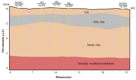
Figure 1.
Stratigraphic profile information of the test area (the yellow dotted frame indicates the drilling profile).
In this study, five test wells were installed at the experimental site (Figure 2), as illustrated in the well layout (Figure 3). Among them, H1 serves as the injection well and H4 as the pumping well, both with depths of 13.1 m. The observation wells—H0 (13.53 m), H2 (13.95 m), and H3 (13.65 m)—are each equipped with screened casing pipes for monitoring purposes. Before the formal tracer test, both a constant-rate pumping test and a stratified micro-hydraulic test were conducted to obtain preliminary hydrogeological parameters. These tests provided reference values for the subsequent numerical model setup, supported estimation of tracer test duration, and enabled initial calibration. Results indicated that the hydraulic conductivities of the aquifers at the site range from 2.585 × 10⁻⁶ to 3.276 × 10⁻⁵ m/s.
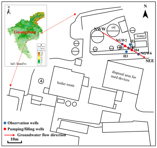
Figure 2.
Plan of the test site.
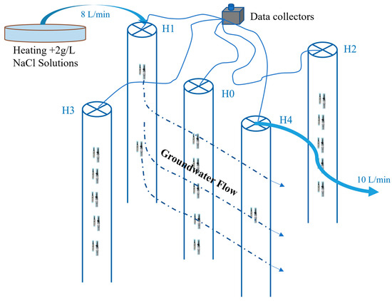
Figure 3.
Schematic diagram of the test well location.
The aquifer is primarily composed of silty clay with low permeability and a weak natural hydraulic gradient. These conditions result in a prolonged tracer migration period and make it difficult to determine a stable flow direction. Additionally, the heterogeneity of the formation becomes more pronounced under such low-gradient conditions, complicating tracer peak detection. To address these challenges and ensure effective parameter inversion, a simultaneous injection and pumping approach was employed. This method establishes a controlled pressure gradient between the injection and pumping wells, promoting directional groundwater flow and enhancing tracer recovery. It also facilitates more accurate characterization of hydrogeological properties while minimizing potential disturbance to the aquifer [42,43,44].
Prior to the coupled tracer test, water level, temperature, and conductivity sensors were installed at a depth of 11.5 m in the pumping well and 12.5 m in the injection well. Additionally, sensor probes were installed at five depths—8.5 m, 9.5 m, 10.5 m, 11.5 m, and 12.5 m—in each of the three observation wells (H0, H2, and H3). These sensors automatically recorded groundwater level, temperature, and electrical conductivity at 1 min intervals throughout the test period. To ensure controlled injection, the injection zone of the injection well was isolated from the upper section using an inflatable packer, effectively confining the injection interval to between 8.3 m and 13.0 m depth. The well structure is shown in Figure 4. The tracer solution was heated using an electric thermostatic heater, and injection commenced only once the target temperature of 313.15 ± 1 K (40 ± 1 °C) was reached to ensure consistent thermal conditions. Tracer injection was performed using a solvent pump at a flow rate of 8 L/min, and the injected volume was recorded continuously. Groundwater was simultaneously extracted from the pumping well using a 250 W clear-water screw pump operating at a flow rate of 8–10 L/min. Due to site limitations, pumping was suspended at night to allow the natural groundwater flow field to recover. The test was conducted in three stages, based on the type of tracer injected: Stage 1 entailed the injection of warm water at 313.15 ± 1 K (40 ± 1 °C) for 17 d. Stage 2 entailed the injection of ambient-temperature water at 298.15 ± 1 K (25 ± 1 °C) for 3 d. Stage 3 entailed the injection of 313.15 ± 1 K (40 ± 1 °C) NaCl solution with conductivity between 2900–3200 μS/cm for 16 d.
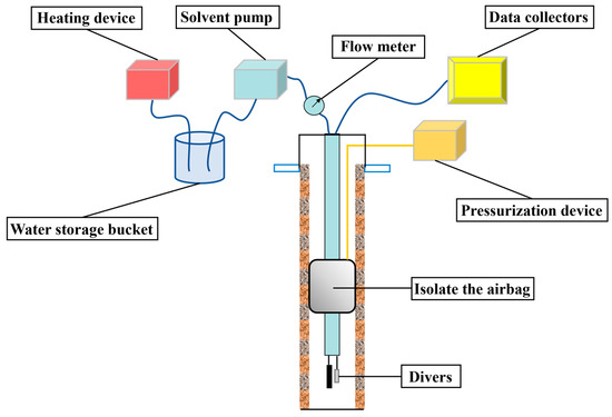
Figure 4.
Schematic structure of the injection well (H1).
A three-dimensional, multiparameter sensor system enabled real-time monitoring of groundwater level, temperature, and solute concentration. The resulting dataset was used as both input and validation criteria for the numerical simulation model described in the following section.
2.2. Conceptual Model
To ensure that pumping activities did not influence boundary water levels or compromise simulation accuracy, the numerical model was centered on the pumping and tracer test area. The horizontal projection area of the three-dimensional model domain is rectangular. The long axis of the numerical simulation domain is 18.55 m and is parallel to the line of the pumping and injection wells. This is the main flow direction of the groundwater flow in the artificial flow field. The short axis is 10.11 m, and the vertical height is 18.67 m. The model was divided vertically into three main layers based on the site stratigraphy and hydrogeological characteristics (as shown in Figure 5). The uppermost layer (0~4 m) represents the fill with a relatively loose structure. The middle layer (4~13.5 m) consists of silty clay and sandy clay and contains the primary test section (8.5~13.5 m). This section is further subdivided into five sublayers, each 1 m thick, to better characterize the vertical heterogeneity during parameter inversion. The bottom layer (13.5~18.67 m) consists of strongly weathered bedrock.
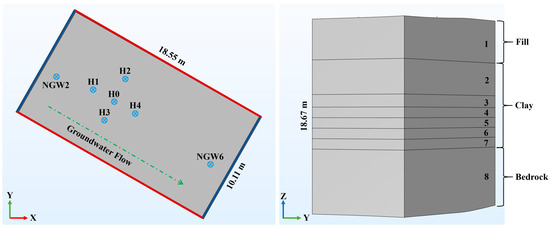
Figure 5.
Numerical model layering diagram.
The initial groundwater level was set according to pre-test measurements. The boundaries along the direction of groundwater flow were assigned zero-flux conditions, while the boundaries perpendicular to the flow direction were set as constant-head boundaries, with head values controlled by long-term observation well data. The model incorporates key hydrogeological parameters, including hydraulic conductivity, thermal conductivity, and solute dispersion coefficient. The hydrogeological conditions in the study area are relatively homogeneous in the horizontal direction; therefore, no horizontal parameter zoning was applied. However, distinct hydrogeological parameter values were assigned to different vertical layers.
2.3. Mathematical Model
The coupled tracer test simulation of the test site in this study mainly uses Darcy’s law, porous media heat transfer, and porous media dilute matter transfer modules; and utilizes the coupling interfaces between the modules to realize the full coupling of the groundwater flow field, temperature field, and solute field.
The control equation for the transient flow state of the Darcy’s law module is as follows:
where t (s) is the time; is the porosity; (kg/m3) is the liquid density; (kg/(m3·s)) is the input mass source; κ (m2) is the permeability; μ (MPa·s) is the kinetic viscosity; ∇p (MPa) is the pressure difference; g (m/s2) is the acceleration of gravity; and u (m/s2) is the flow rate of groundwater.
The control equation of the module for heat transfer in porous media is as follows:
where (J/(kg·K)) is the constant pressure heat capacity of the fluid; (kg/m3) is the fluid density; T (K) is the Kelvin temperature; Q (J) is the heat source term; q (W/m2) is the heat flux; and (W/(m·K)) is the effective thermal conductivity.
In this study, the tracer concentration was low, and the dilute solute transfer module in porous media was chosen to simulate salt transport. The control equation for the dilute solute transfer module in porous media was as follows:
where (kg/m3) is the density of the fluid; (mol/m3) is the concentration of the dilute substance; t (s) is the time; (m/s) is the velocity vector of the fluid; (m2/s) is the diffusion coefficient of the dilute substance; and (mol/(s·m3)) is the source term.
2.4. Numerical Model
In this study, a three-dimensional groundwater flow model was developed using the finite element software COMSOL Multiphysics 6.2. To ensure the accuracy and stability of the numerical simulation, a mesh independence analysis was conducted. Mesh density and cell size were adjusted using the built-in mesh refinement levels available in COMSOL. Prior to finalizing the mesh, several refinement levels were systematically tested. For each case, the Root Mean Square Error (RMSE) between simulated and observed groundwater levels at the monitoring wells, along with computational time, was evaluated to determine the optimal mesh configuration. The mesh parameters and corresponding evaluation results are presented in Figure 6. Based on a comparison of RMSE values, average mesh quality, and simulation time, the optimal mesh refinement level was selected. The final mesh consisted of 15,813 cells.
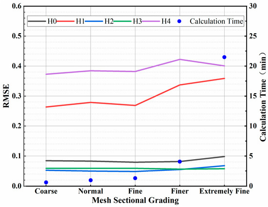
Figure 6.
Plot of RMSE, calculation time vs. grid dissection.
Initial and boundary conditions were assigned according to the conceptual model and field observations. Boundaries perpendicular to the main direction of groundwater flow were defined as constant-head boundaries, with head values controlled by real-time water level data from observation wells NGW2 and NGW6. Boundaries parallel to the flow direction were set as no-flow boundaries due to the relatively low hydraulic gradient in that direction. The top and bottom surfaces were also designated as no-flow boundaries. In the heat-transfer module, the initial temperature at 8.5 m depth was set to 298.45 K, and a linear adjustment of ±0.03 K/m was applied vertically. This entailed an increase of 0.03 K/m above 8.5 m and a decrease of 0.03 K/m below it. The vertical sides of the domain were modeled as convective heat flux boundaries, while the top and bottom were assigned thermal insulation conditions. The injection well was treated as a line heat source. In the solute transport module, the initial NaCl concentration was set to 0 mol/m3. The top and bottom boundaries were defined as no-flux boundaries, and the lateral sides were modeled as open boundaries, allowing for solute free diffusion. The injection well was represented as a time-dependent line mass source, with injection flux controlled by a piecewise function.
2.5. Inversion of Hydrogeological Parameters
The inversion of hydrogeological parameters in this investigation was executed using a trial-and-error methodology, leveraging observed data pertaining to groundwater level, temperature, and NaCl concentration obtained during the tracer test. The inversion framework consisted of three sequential stages: (1) calibration of the groundwater flow model, (2) validation of the coupling model, and (3) adjustment of the hydrothermal salt coupling model. Initially, the hydraulic conductivity of the aquifer was modified to reduce discrepancies between the simulated and observed water levels across multiple observation wells. This calibrated hydraulic conductivity was subsequently employed as an input for both the hydrothermal coupling model and the hydro-salt coupling model to validate the thermal conductivity and dispersion coefficient, respectively. In cases where significant deviations were noted between the simulated temperature or concentration and the observed values, the parameters underwent iterative adjustments. Ultimately, three parameters—hydraulic conductivity, thermal conductivity, and dispersion coefficient—were incorporated into the hydrothermal salt coupling for final refinement. This iterative process was repeated until the three observed outputs (groundwater level, temperature, and NaCl concentration) demonstrated a satisfactory alignment with the simulation results. This multiphase calibration approach facilitated a robust and reliable inversion of hydrogeological parameters.
The inversion of hydrogeological parameters for the target aquifer was based on monitoring data collected during the field tests, including groundwater level, temperature, and solute concentration. The reliability of the model was evaluated by comparing simulated results with observed values at the monitoring wells, and calibration accuracy was assessed using the RMSE as a quantitative metric.
where “” represents the value obtained from numerical simulations, “” indicates the corresponding actual measured value, and “” denotes the total number of sampling points. The RMSE serves as an essential metric for evaluating the accuracy of data fitting results. A lower RMSE signifies a greater correspondence between the simulated outcomes and the actual measurements.
The overarching framework of inversion can be delineated into three fundamental stages: the identification of the groundwater flow model, which serves as the basis for parameter inversion; the establishment of the hydrothermal and hydro-salt coupling model, which functions as the verification mechanism for the parameter inversion; and the formulation of the hydrothermal salt coupling model, which acts as the adjustment phase for the parameter inversion. Initially, the parameters associated with the groundwater flow model are determined, leading to the inversion of a set of hydraulic conductivities that align with the groundwater flow model by fitting the water levels recorded at each observation well. This set of hydraulic conductivities is then integrated into the hydrothermal and hydro-salt coupling model, where a corresponding set of thermal conductivity coefficients and dispersion coefficients is inverted by fitting the temperature data from each observation well and the solute concentration measurements. Subsequently, the thermal conductivity and dispersion coefficients are refined through the identification of the two coupled models. Ultimately, the inverted hydrogeological parameters—namely, the hydraulic conductivity, thermal conductivity coefficient, and dispersion coefficient—are incorporated into the hydrothermal salt coupling model for further adjustment, with the aim of enhancing accuracy through the comprehensive identification of the entire coupling model. Should the parameter validation process prove inadequate (e.g., if the temperature and solute concentration curves do not align), the aquifer parameters within the groundwater flow model will be subject to adjustment and re-inversion. Through iterative processes, hydrogeological parameters that satisfy both the groundwater flow model and the coupled model are ultimately derived. The concurrent identification of the groundwater flow model and the coupled model facilitates the reliable inversion of hydrogeological parameters.
3. Results and Discussion
3.1. Analysis of Groundwater Flow Field Simulation Results
This section focuses on the simulation of the Darcy flow field at the test site, calibrated using water level data collected from each observation well. The hydraulic conductivities of the aquifer were obtained through preliminary parameter inversion, and the hydraulic parameter settings for each model layer are summarized in Table 1.

Table 1.
Hydrogeological parameters of model layers used in the initial simulation.
As illustrated in Figure 7, the simulated groundwater levels in observation wells H0, H2, and H3 show good agreement with the measured data when a time step of 1 min and a total simulation duration of 1.667 d are used. The RMSE values are 0.0972 for H0, 0.0667 for H2, and 0.0584 for H3. The slightly higher RMSE for H0 is attributed to its location along the axis connecting the injection and pumping wells, where greater hydraulic fluctuations occur. The RMSE for the injection well H1 is 0.3370, primarily due to structural differences between the actual injection well and its representation in the model. In the field, a spigot and fire hose assembly were used to control the injection depth, and the hose’s internal diameter was smaller than that of the injection well casing. As a result, the water level measured by the sensor within the injection well was artificially elevated, leading to discrepancies between observed and simulated values. The largest RMSE value (0.3530) was observed for the pumping well H4. This deviation is largely attributed to unsteady pumping rates during the test. Although the simulation employed average flow rates over different time intervals, the real-time variations in pumping were not fully captured. Consequently, the flow rate input in the model deviated significantly from actual values over short periods, resulting in a mismatch between simulated and observed water levels at H4.
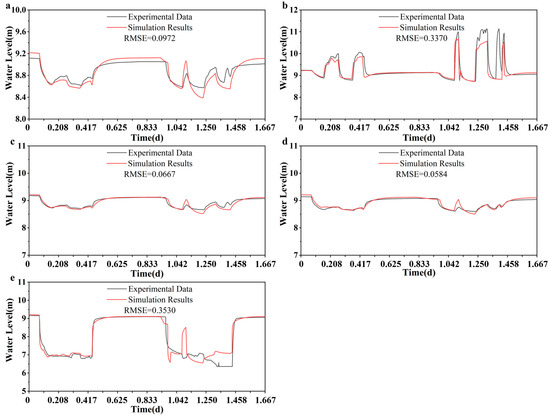
Figure 7.
Comparison of experimental and simulated values of water levels in observation and test wells: (a) H0, (b) H1, (c) H2, (d) H3, and (e) H4.
Despite some local discrepancies, the overall calibration of groundwater levels is satisfactory, indicating that the model parameters are reasonably configured and capable of accurately simulating the groundwater flow field at the study site.
3.2. Analysis of Hydrothermal Coupling Results
In this section, the temperature field is integrated with the developed groundwater flow model, and the thermal conductivity coefficient of the model layer is determined through fitting temperature data from observation wells, leading to an inversion process. The simulation results for temperature at various depths of the observation wells are illustrated in Figure 8 and Figure 9, with the parameter configurations detailed in Table 2. It is noted that the temperature variation recorded at observation well H3 is minimal, and the temperature changes predicted by the model exhibit little fluctuation. Therefore, the subsequent discussion will concentrate solely on the findings from wells H0 and H2.
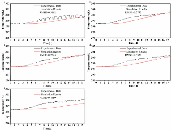
Figure 8.
Comparison of experimental and simulated values of temperature at different depths in the observation well H0: (a) 8.5 m, (b) 9.5 m, (c) 10.5 m, (d) 11.5 m, and (e) 12.5 m.
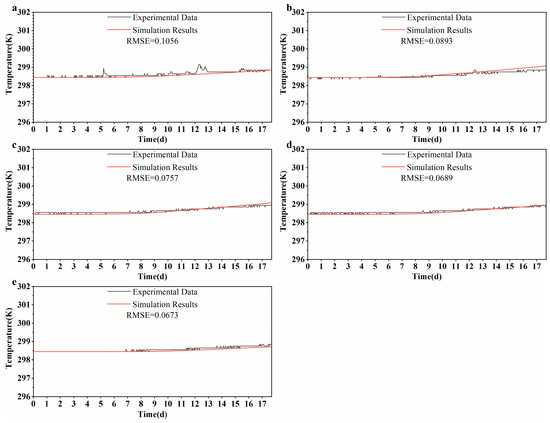
Figure 9.
Comparison of experimental and simulated values of temperature at different depths in the observation well H2: (a) 8.5 m, (b) 9.5 m, (c) 10.5 m, (d) 11.5 m, and (e) 12.5 m.
Table 2.
Parameters of porous media heat-transfer module.
As shown in Figure 8 and Figure 9, the simulated temperature trends at multiple depths generally align with the observed data from wells H0 and H2. In particular, at depths of 9.5 m, 10.5 m, and 11.5 m, both the magnitude and rate of temperature increase are more pronounced, reflecting a strong thermal response to warm water injection. This pattern is consistent with enhanced convective heat transfer and the propagation of thermal fronts at mid-depths. At 8.5 m in well H0, greater fluctuations in observed temperature are likely caused by near-surface atmospheric influences, which the model does not fully capture. Meanwhile, the 12.5 m layer displays slower warming and greater deviation from the simulated curve, potentially due to low hydraulic connectivity and limited heat transport. In contrast, well H2 shows lower RMSE values and closer agreement with simulation outputs, suggesting that heat transfer in this well is predominantly governed by conduction, as indicated by the relatively smooth temperature curves.
3.3. Analysis of Hydro-Salt Coupling Results
The solute transport model was subsequently integrated with the groundwater flow model. The longitudinal dispersion coefficient of the model layer was inverted using observed NaCl concentration data from the monitoring wells. The estimated values of dispersion and diffusion coefficients are summarized in Table 3.
Table 3.
Parameter settings for the rare-substance-transfer module.
Figure 10 and Figure 11 present a comparison between measured and simulated NaCl concentrations at various depths in wells H0 and H2. Sodium chloride injection commenced on day 22. Due to low initial NaCl concentrations and the presence of background groundwater conductivity, early-stage breakthrough was difficult to detect. Consequently, simulated concentrations at H0 from days 22 to 25 showed noticeable deviations—particularly at depths of 9.5 m, 10.5 m, and 11.5 m—with RMSE values exceeding 0.34, indicating moderate model performance. From day 25 onward, the model more accurately reproduced observed data, likely due to the clearer breakthrough signal as background noise diminished. At 12.5 m, simulated concentrations remained low, potentially because the model did not account for vertical wellbore mixing or the full complexity of miscible transport within the well column. In well H2, the agreement between observed and simulated NaCl concentrations improved, with RMSE values generally below 0.31. This improvement may be attributed to reduced background conductivity interference and more stable hydrogeological conditions at the H2 location. Notably, even a slight increase in background conductivity—from 447 to 565 μS/cm—demonstrates the sensitivity of tracer-based inversion results to initial site-specific conditions. These findings highlight the importance of accurately characterizing background hydro-chemical conditions when conducting solute transport modeling.
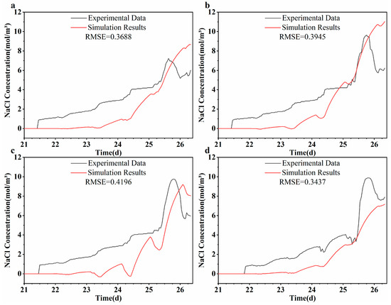
Figure 10.
Comparison of experimental and simulated values of NaCl concentration at different depths in the observation well H0: (a) 9.5 m, (b) 10.5 m, (c) 11.5 m, and (d) 12.5 m.
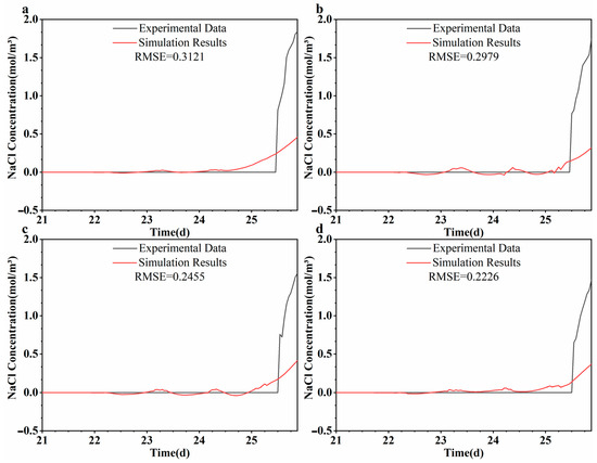
Figure 11.
Comparison of experimental and simulated values of NaCl concentration at different depths in the observation well H2: (a) 9.5 m, (b) 10.5 m, (c) 11.5 m, and (d) 12.5 m.
3.4. Analysis of Hydrothermal Salt Coupling Results
This section presents a fully coupled simulation of the groundwater flow, temperature, and solute transport fields, incorporating the hydraulic conductivity, thermal conductivity, and dispersion coefficients obtained through previous inversion processes. The simulation results are compared against those from the hydrothermal and hydro-salt coupling models to analyze the interactions among the three physical fields.
As illustrated in Figure 12 and Figure 13, the simulated values of the hydrothermal salt coupling temperature at different depths of observation wells H0 and H2 are higher than the simulated values of the hydrothermal coupling temperature. Since the specific heat capacity of groundwater becomes smaller as the concentration of NaCl in groundwater increases, the heat required for groundwater to rise to the same temperature decreases. However, the concentration of NaCl in this test is lower; therefore, the temperature increase is smaller. The difference between the simulated value of the hydrothermal salt coupling temperature and the simulated value of the hydrothermal coupling temperature began to increase on the 24th day of the test, and the temperature difference is particularly pronounced at depths of 9.5 m and 10.5 m. The enhancement in temperature at these depths is likely due to the presence of preferential flow paths, where increased permeability and higher NaCl concentrations promote rapid thermal propagation. In contrast, temperature differences at other depths are less significant. Additionally, the greater overall thermal response observed in well H0, which is aligned with the injection–pumping axis, reflects its exposure to stronger groundwater flow and heat transport relative to well H2.
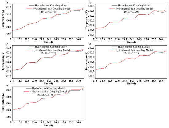
Figure 12.
Comparison of simulated temperature values at different depths of the observation well H0 in hydrothermal coupling and hydrothermal-salt coupling: (a) 8.5 m, (b) 9.5 m, (c) 10.5 m, (d) 11.5 m, and (e) 12.5 m.
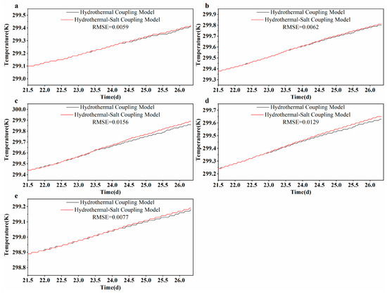
Figure 13.
Comparison of simulated temperature values at different depths of the observation well H2 in hydrothermal coupling and hydrothermal-salt coupling: (a) 8.5 m, (b) 9.5 m, (c) 10.5 m, (d) 11.5 m, and (e) 12.5 m.
These results indicate that the hydrothermal-salt model exhibits greater sensitivity to temperature variations than the hydrothermal model, particularly in mid-depth strata. The influence of salinity on reducing the specific heat capacity of groundwater, coupled with convection-enhanced heat transfer, accelerates thermal breakthrough. The depth-dependent differences further reflect subsurface heterogeneity in permeability and lithology.
Figure 14 and Figure 15 illustrate a comparative analysis of the NaCl concentrations predicted by the water-salt coupling model and the hydrothermal-salt coupling model at various depths within wells H0 and H2. Throughout all examined depths, the hydrothermal-salt model consistently forecasts elevated NaCl concentrations, thereby substantiating the thermal effects in accelerating solute transport. This divergence becomes increasingly pronounced during the subsequent simulation phase (Days 24–26). Quantitatively, the average concentration increase across all depths in well H0 is approximately 2.5 mol/m3, whereas in well H2, it is 0.7 mol/m3. The thermal influence has been demonstrated to decrease fluid viscosity, increase groundwater velocity, and augment convective transport, particularly along the injection-pumping axis where well H0 is situated. Consequently, this leads to an earlier tracer breakthrough in the hydrothermal-salt model, occurring approximately 5 h earlier in H0 and 17 h earlier in H2. This illustrates the impact of thermal conditions on transport kinetics. Additionally, at a depth of 12.5 m in well H2, the enhancement is minimal, suggesting low vertical permeability and limited thermal convection. This observation supports the hypothesis of stratified flow and vertical heterogeneity within the lithology of the site. The simulation outcomes indicate that the integration of thermal effects significantly improves the precision of solute transport modeling within coupled physical fields.
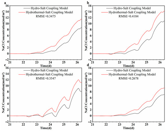
Figure 14.
Comparison of simulated values of NaCl concentration at different depths of the observation well H0 in hydro-salt coupling and hydrothermal-salt coupling: (a) 9.5 m, (b) 10.5 m, (c) 11.5 m, and (d) 12.5 m.
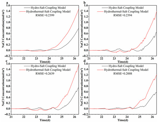
Figure 15.
Comparison of simulated values of NaCl concentration at different depths of the observation well H2 in hydro-salt coupling and hydrothermal-salt coupling: (a) 9.5 m, (b) 10.5 m, (c) 11.5 m, and (d) 12.5 m.
When contrasted with the water-salt model, the hydrothermal-salt coupling model exhibits a more significant and expedited response in the transport of NaCl. This effect can be explained by the decrease in viscosity resulting from variations in temperature, alongside an enhancement in groundwater mobility. The differences observed in concentration, breakthrough time, and sensitivity at various depths offer compelling evidence for the presence of stratified flow and heterogeneous permeability within the study area.
The hydraulic conductivities for each layer within the test section were modified in response to the fluctuations in temperature and conductivity observed in each layer (refer to Table 4). This methodology was implemented to enhance the accuracy of the aquifer representation. The effectiveness of these modifications was primarily assessed through the variations in the RMSE associated with the water level calculation values for each test well after the parameter adjustments were made. The results of the groundwater level simulations in the test wells subsequent to these adjustments are illustrated in Figure 16.
Table 4.
Parameter settings utilized for testing layers.
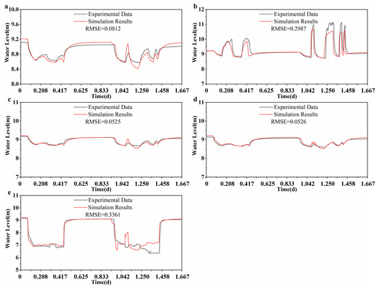
Figure 16.
Comparison of experimental and simulated values of water levels in observation and test wells after parameter adjustment: (a) H0, (b) H1, (c) H2, (d) H3, and (e) H4.
As illustrated in Figure 16, the simulated water level values in the individual test wells are closer to the measured values after adjusting the hydraulic conductivity to the temperature signal, and the RMSEs are all reduced. The above results show that in the parameter adjustment, the use of other signals of spatial and temporal distribution characteristics can enhance model refinement and parameter accuracy. At the same time, it also shows that, compared to the traditional hydrogeological tests, the coupled tracer test with a variety of signals can be a better way to obtain the aquifer parameters.
Overall, the fit between the modeling results and the observed data shows that the model can better reflect the actual hydrogeological conditions. Overall, the values of the parameters correspond to the empirical range, and the values of the hydrogeological parameters of the pumped aquifer are similar to those calculated by the analytical method. The hydrogeological parameters of the silt layer derived from the final inversion are as follows: target aquifer permeability coefficient K = 6.72~8.52 × 10⁻⁶ m/s; the longitudinal thermal conductivity, transverse thermal conductivity, and vertical thermal conductivity are 2.2, 0.45, and 1.25 W/(m·K), respectively; and the vertical and lateral dispersions of the target aquifer are 0.554 m and 0.05 m.
4. Conclusions
The current research employs a site-scale coupled tracer test to evaluate changes in groundwater levels throughout the duration of the site assessment, alongside the collection of temperature and conductivity data at various depths over time. In parallel, a numerical simulation is conducted to model groundwater flow, temperature, and solute concentration within the test area during the experiment. This modeling is facilitated through the use of the COMSOL Multiphysics 6.2 finite element software, which is instrumental in determining the hydraulic conductivity, thermal conductivity coefficient, and dispersion coefficient of the aquifer. The methodology also allows for the exploration of interactions among different physical fields. Additionally, three-dimensional spatial data on temperature are utilized to accurately characterize the hydraulic conductivity of the test aquifer. The analyses yield the following specific conclusions:
- (1)
- A comprehensive three-dimensional multiparameter monitoring platform was established at the site, which facilitated the simultaneous measurement of water level, temperature, and conductivity. This platform was also utilized for a coupled water-heat-salt tracer test. During the testing phase, extensive multilevel time-series data were collected, encompassing groundwater level, temperature, and conductivity measurements in observation wells. Notably, the initial alterations in temperature and conductivity were detected in the stratum located at a burial depth of 9 to 11 m, suggesting a significant hydraulic conductivity within the formation at this specific depth.
- (2)
- The RMSE between the simulated water levels in observation wells and the test values derived from the single groundwater flow model is minimal, suggesting a more precise representation of the groundwater flow field and an accurate inversion of the aquifer’s hydraulic conductivity. In the coupled hydrothermal-salt model, the test section is stratified to account for the influences of temperature and solute concentration (specifically NaCl), leading to adjustments in the hydraulic conductivities of the various layers. As a result, the hydraulic conductivity that reflects hydrothermal-salt interactions is determined. Furthermore, the RMSE between the water level data from the observation wells during the coupled tracer test and the simulated values from the coupled model is significantly reduced, indicating a more refined portrayal of the aquifer and enhanced accuracy in the hydraulic conductivities obtained through inversion.
- (3)
- Based on the experimental platform to obtain data on pollutant migration and transformation under the influence of three-dimensional multifield coupling and the numerical model of multiphysical field coupling, physical and numerical simulation experiments on seepage and solvent transport are carried out under the coupling of different physical fields. The inversion results for the hydraulic conductivity of the target aquifer range from 6.72 × 10⁻⁶ m/s to 8.52 × 10⁻⁶ m/s, with the effective thermal conductivity of 2.2 W/(m·K), the longitudinal diffusivity of 0.554 m, and the transverse dispersion of 0.05 m.
- (4)
- The coupling between the temperature field and solute concentration field arises from the effect of temperature on the salt diffusion coefficient. Changes in temperature influence the salt diffusion coefficient, thereby affecting the rate of salt transport and the degree of dispersion. During the transport of dissolved substances in groundwater, heat is also released or absorbed by the salt transport. Higher salt concentrations in groundwater reduce the specific heat capacity of the groundwater, leading to faster temperature changes.
Author Contributions
J.Y.: software, experiment, formal analysis, writing—original draft. C.C.: conceptualization methodology, software and validation. G.H.: formal analysis, writing—review and editing, validation. J.H.: software, experiment, formal analysis. Z.C.: conceptualization, validation, writing—original draft, writing—review and editing, visualization. All authors have read and agreed to the published version of the manuscript.
Funding
This work was supported by the National Key R&D Program of China (grant number 2023YFC3706004); the National Natural Science Foundation of China (grant number 42377079); and the Jiangsu Provincial Natural Science Foundation General Project (grant number BK20221507).
Data Availability Statement
The original contributions presented in this study are included in the article. Further inquiries can be directed to the corresponding authors.
Conflicts of Interest
Author Changsheng Chen was employed by the company Changjiang Survey Planning Design and Research, Co., Ltd. The remaining authors declare that the research was conducted in the absence of any commercial or financial relationships that could be construed as a potential conflict of interest.
References
- Cusano, D.; Coda, S.; De Vita, P.; Fabbrocino, S.; Fusco, F.; Lepore, D.; Nicodemo, F.; Pizzolante, A.; Tufano, R.; Allocca, V. A comparison of methods for assessing groundwater vulnerability in karst aquifers: The case study of Terminio Mt. aquifer (Southern Italy). Sustain. Environ. Res. 2023, 33, 42. [Google Scholar] [CrossRef]
- Ma, J.; Li, D.; Wang, M. The Evaluation of the Hydrogeological Parameters of a Field Pumping Test within Multi-layer Unconfined Pebble Aquifers: A Case Study. Ksce J. Civ. Eng. 2021, 25, 4018–4031. [Google Scholar] [CrossRef]
- Li, P.; Qian, H.; Wu, J. Comparison of three methods of hydrogeological parameter estimation in leaky aquifers using transient flow pumping tests. Hydrol. Process. 2014, 28, 2293–2301. [Google Scholar] [CrossRef]
- Demichele, F.; Micallef, F.; Portoghese, I.; Mamo, J.A.; Sapiano, M.; Schembri, M.; Schueth, C. Determining Aquifer Hydrogeological Parameters in Coastal Aquifers from Tidal Attenuation Analysis, Case Study: The Malta Mean Sea Level Aquifer System. Water 2023, 15, 177. [Google Scholar] [CrossRef]
- Xu, Q.; Wang, G.; Liang, X.; Qu, S.; Shi, Z.; Wang, X. Determination of Mining-Induced Changes in Hydrogeological Parameters of Overburden Aquifer in a Coalfield, Northwest China: Approaches Using the Water Level Response to Earth Tides. Geofluids 2021, 2021, 5516997. [Google Scholar] [CrossRef]
- Mejia, N.; Scheytt, T.J.; Murillo, M. Hydrogeological characterization and utilization of the Siguatepeque aquifer, Honduras. Hydrogeol. J. 2024, 32, 557–575. [Google Scholar] [CrossRef]
- Srzic, V.; Lovrinovic, I.; Racetin, I.; Pletikosic, F. Hydrogeological Characterization of Coastal Aquifer on the Basis of Observed Sea Level and Groundwater Level Fluctuations: Neretva Valley Aquifer, Croatia. Water 2020, 12, 348. [Google Scholar] [CrossRef]
- Zhang, H.; Shi, Z.; Wang, G.; Yan, X.; Liu, C.; Sun, X.; Ma, Y.; Wen, D. Different Sensitivities of Earthquake-Induced Water Level and Hydrogeological Property Variations in Two Aquifer Systems. Water Resour. Res. 2021, 57, e2020WR028217. [Google Scholar] [CrossRef]
- Cardiff, M.; Barrash, W. Analytical and Semi-Analytical Tools for the Design of Oscillatory Pumping Tests. Groundwater 2015, 53, 896–907. [Google Scholar] [CrossRef]
- Yu, X.; Zhang, J.; Miao, D. Innovative Closure Law for Pump-Turbines and Field Test Verification. J. Hydraul. Eng. 2015, 141, 05014010. [Google Scholar] [CrossRef]
- Zech, A.; Attinger, S. Technical note: Analytical drawdown solution for steady-state pumping tests in two-dimensional isotropic heterogeneous aquifers. Hydrol. Earth Syst. Sci. 2016, 20, 1655–1667. [Google Scholar] [CrossRef]
- Chen, J.-L.; Wen, J.-C.; Yeh, T.-C.J.; Lin, K.-Y.A.; Wang, Y.-L.; Huang, S.-Y.; Ma, Y.; Yu, C.-Y.; Lee, C.-H. Reproducibility of hydraulic tomography estimates and their predictions: A two-year case study in Taiwan. J. Hydrol. 2019, 569, 117–134. [Google Scholar] [CrossRef]
- Huang, S.-Y.; Wen, J.-C.; Yeh, T.-C.J.; Lu, W.; Juan, H.-L.; Tseng, C.-M.; Lee, J.-H.; Chang, K.-C. Robustness of joint interpretation of sequential pumping tests: Numerical and field experiments. Water Resour. Res. 2011, 47, W10530. [Google Scholar] [CrossRef]
- Zech, A.; Mueller, S.; Mai, J.; Hesse, F.; Attinger, S. Extending Theis’ solution: Using transient pumping tests to estimate parameters of aquifer heterogeneity. Water Resour. Res. 2016, 52, 6156–6170. [Google Scholar] [CrossRef]
- Deng, R.; Wu, D.; Zhao, S. Numerical simulation of ground and groundwater factors affecting NMR probe. Desalination Water Treat. 2018, 121, 118–125. [Google Scholar] [CrossRef]
- Dong, L.; Luo, Z.; Guo, H.; Cheng, L.; Wang, X.; Zhao, Q. The impact of developing a regional multiwell groundwater heat pump system on the geological environment: A case study in Haimen, China. Hydrogeol. J. 2025, 33, 257–277. [Google Scholar] [CrossRef]
- Hayley, K. The Present State and Future Application of Cloud Computing for Numerical Groundwater Modeling. Groundwater 2017, 55, 678–682. [Google Scholar] [CrossRef]
- Miao, T.; Guo, J. Application of artificial intelligence deep learning in numerical simulation of seawater intrusion. Environ. Sci. Pollut. Res. 2021, 28, 54096–54104. [Google Scholar] [CrossRef]
- Szabó, N.P. A genetic meta-algorithm-assisted inversion approach: Hydrogeological study for the determination of volumetric rock properties and matrix and fluid parameters in unsaturated formations. Hydrogeol. J. 2018, 26, 1935–1946. [Google Scholar] [CrossRef]
- Moharir, K.; Pande, C.; Patil, S. Inverse modelling of aquifer parameters in basaltic rock with the help of pumping test method using MODFLOW software. Geosci. Front. 2017, 8, 1385–1395. [Google Scholar] [CrossRef]
- Tang, L.; Cheng, Z.; Li, G.; Chen, Y.; Wang, Y. Permeability coefficient of waterproof curtain by borehole packer test. J. Hydrol. 2023, 625, 130023. [Google Scholar] [CrossRef]
- Wagner, V.; Bayer, P.; Bisch, G.; Kuebert, M.; Blum, P. Hydraulic characterization of aquifers by thermal response testing: Validation by large-scale tank and field experiments. Water Resour. Res. 2014, 50, 71–85. [Google Scholar] [CrossRef]
- Scorpo, A.L.; Nordell, B.; Gehlin, S. A Method to Estimate the Hydraulic Conductivity of the Ground by TRT Analysis. Groundwater 2017, 55, 110–118. [Google Scholar] [CrossRef] [PubMed]
- Qi, C.; Zhou, R.; Zhan, H. Analysis of heat transfer in an aquifer thermal energy storage system: On the role of two-dimensional thermal conduction. Renew. Energy 2023, 217, 119156. [Google Scholar] [CrossRef]
- Canul-Macario, C.; Gonzalez-Herrera, R.; Sanchez-Pinto, I.; Graniel-Castro, E. Contribution to the evaluation of solute transport properties in a karstic aquifer (Yucatan, Mexico). Hydrogeol. J. 2019, 27, 1683–1691. [Google Scholar] [CrossRef]
- List, E.J. Contaminant Dispersion and Breakthrough in Groundwater Flow: Case Study in Maui, Hawaii. J. Hydraul. Eng. 2022, 148, 05022006. [Google Scholar] [CrossRef]
- Yan, C.; Xie, X.; Ren, Y.; Ke, W.; Wang, G. A FDEM-based 2D coupled thermal-hydro-mechanical model for multiphysical simulation of rock fracturing. Int. J. Rock Mech. Min. Sci. 2022, 149, 104964. [Google Scholar] [CrossRef]
- Beyer, C.; Popp, S.; Bauer, S. Simulation of temperature effects on groundwater flow, contaminant dissolution, transport and biodegradation due to shallow geothermal use. Environ. Earth Sci. 2016, 75, 1244. [Google Scholar] [CrossRef]
- Huang, J.; Zhang, C. Role of Temperature and Flow in Biomass Transporting in Porous Media. In Proceedings of the 2nd International Conference on Civil Engineering, Architecture and Building Materials (CEABM 2012), Yantai, China, 25–27 May 2012; pp. 80–87. [Google Scholar]
- Wei, Y.; Chen, Y.; Cao, X.; Xiang, M.; Huang, Y.; Li, H. A Critical Review of Groundwater Table Fluctuation: Formation, Effects on Multifields, and Contaminant Behaviors in a Soil and Aquifer System. Environ. Sci. Technol. 2024, 58, 2185–2203. [Google Scholar] [CrossRef]
- Chen, Z.-G.; Tang, C.-S.; Shen, Z.; Liu, Y.-M.; Shi, B. The geotechnical properties of GMZ buffer/backfill material used in high- level radioactive nuclear waste geological repository: A review. Environ. Earth Sci. 2017, 76, 270. [Google Scholar] [CrossRef]
- Cuiuli, E.; Procopio, S. Hydrogeological Survey, Radiometric Analysis and Field Parametric Measurements: A Combined Tool for the Study of Porous Aquifers. Water 2022, 14, 2173. [Google Scholar] [CrossRef]
- Barlebo, H.C.; Hill, M.C.; Rosbjerg, D. Investigating the Macrodispersion Experiment (MADE) site in Columbus, Mississippi, using a three-dimensional inverse flow and transport model. Water Resour. Res. 2004, 40, W04211. [Google Scholar] [CrossRef]
- Bowling, J.C.; Zheng, C.M.; Rodriguez, A.B.; Harry, D.L. Geophysical constraints on contaminant transport modeling in a heterogeneous fluvial aquifer. J. Contam. Hydrol. 2006, 85, 72–88. [Google Scholar] [CrossRef] [PubMed]
- Qiao, X.; Xiao, P.; Wang, J.; Li, J.; Wang, L. Reconstruction project of Zhengzhou groundwater balance experiment site: Promotion of the key application problems of experiment site monitoring data. Hydrogeol. Eng. Geol. 2020, 47, 46–52. [Google Scholar]
- Chen, Z.; Yue, R.; Liu, L.; Yin, L.; Mao, X. Modeling of the heat transfer of in-situ electrical resistance heating remediation and numerical simulation. Chin. J. Environ. Eng. 2022, 16, 2653–2662. [Google Scholar]
- Rastorguev, I.A. Two-Dimensional Flow and Mass Transport through Variably Saturated Porous Media from a Surface Waste Storage. Water Resour. 2020, 47, 211–221. [Google Scholar] [CrossRef]
- Karmakar, S.; Tatomir, A.; Oehlmann, S.; Giese, M.; Sauter, M. Numerical Benchmark Studies on Flow and Solute Transport in Geological Reservoirs. Water 2022, 14, 1310. [Google Scholar] [CrossRef]
- Jafari, A.; Vahab, M.; Broumand, P.; Khalili, N. An eXtended finite element method implementation in COMSOL multiphysics: Thermo-hydro-mechanical modeling of fluid flow in discontinuous porous media. Comput. Geotech. 2023, 159, 105458. [Google Scholar] [CrossRef]
- Zlotnik, V.; Rabinovich, A.; Cardiff, M. The Bredehoeft problem: Evaluating salvage during groundwater pumping in unconfined aquifers. J. Hydrol. 2024, 637, 131293. [Google Scholar] [CrossRef]
- Mohamed, Y.S.; Hozien, O.; Sorour, M.M.; El-Maghlany, W.M. Heat transfer simulation of nanofluids heat transfer in a helical coil under isothermal boundary conditions using COMSOL multiphysics. Int. J. Therm. Sci. 2023, 192, 108396. [Google Scholar] [CrossRef]
- Colombani, N.; Giambastiani, B.M.S.; Mastrocicco, M. Combined use of heat and saline tracer to estimate aquifer properties in a forced gradient test. J. Hydrol. 2015, 525, 650–657. [Google Scholar] [CrossRef]
- Ptak, T.; Piepenbrink, M.; Martac, E. Tracer tests for the investigation of heterogeneous porous media and stochastic modelling of flow and transport—A review of some recent developments. J. Hydrol. 2004, 294, 122–163. [Google Scholar] [CrossRef]
- Qiao, F.; Wang, J.; Chen, Z.; Zheng, S.; Kwaw, A.K.; Zhao, Y.; Huang, J. Experimental research on the transport-transformation of organic contaminants under the influence of multi-field coupling at a site scale. J. Hazard. Mater. 2024, 470, 134222. [Google Scholar] [CrossRef] [PubMed]
Disclaimer/Publisher’s Note: The statements, opinions and data contained in all publications are solely those of the individual author(s) and contributor(s) and not of MDPI and/or the editor(s). MDPI and/or the editor(s) disclaim responsibility for any injury to people or property resulting from any ideas, methods, instructions or products referred to in the content. |
© 2025 by the authors. Licensee MDPI, Basel, Switzerland. This article is an open access article distributed under the terms and conditions of the Creative Commons Attribution (CC BY) license (https://creativecommons.org/licenses/by/4.0/).