Abstract
This study analyzed the impact of land use and cover changes, along with climate variability, on water consumption by quantifying actual evapotranspiration () in the Tres Cruces River basin (TCR) in Uruguay. Using Landsat 8 and 9 images from 2014 to 2024, the SAFER method (Simple Algorithm for Evapotranspiration Retrieving), applied for the first time in Uruguay, estimated for natural vegetation (grasslands and riparian forests) and commercial afforestation areas. Quality metrics, including determination coefficient (r2 = 0.87), Pearson correlation (r = 0.94), root mean square error (RMSE = 1.46 mm/day), and Nash–Sutcliffe efficiency (NSE = 0.34), were utilized for SAFER’s optimal parameterization based on the literature. Results revealed monthly variability and highlighted higher values for afforestation areas, exceeding grasslands by 26.5% and riparian forests by 4.79%, reflecting increased water demand due to greater biomass and photosynthetic activity. Additionally, prolonged drought periods correlated with increased water consumption by forest vegetation, despite the Standardized Precipitation-Evapotranspiration Index (SPEI) remaining within normal bounds during the 2020–2023 drought. These findings underscore the significant hydrological implications of converting grasslands to afforestation and the need for integrated water resource management amid expanding commercial forestry in the region.
1. Introduction
The increasing demand for water, driven by climate and management practices, and the intensification of droughts highlight the urgency of addressing supply and demand dynamics. This implies that hydrological studies should focus on the demand for water, particularly evapotranspiration (ET), to reverse the situation; most studies have focused mainly on the supply side of the water equation [1].
The accurate estimation of ET across spatial and temporal scales is fundamental for water resource management. ET directly influences key hydrological processes, including water consumption assessment in diverse land-use systems, crop water productivity analysis, agricultural drought monitoring, water balance studies, and climate change adaptation strategies [2].
At small scales, several methods and instruments for determining ET have been developed over time, such as weighing lysimeters, the Penman–Monteith equation, and the Eddy covariance method, among others. However, these methods are generally complex, expensive, and often limited to academic and research settings. For large scales, satellite remote sensing methods can provide reliable information and determine the spatial distribution of ET. Although some satellite missions do not fully meet all the requirements for comprehensive ET-based science and applications, recent advances have improved their capabilities [1,3,4,5].
Recent progress in Earth observation platforms, alongside the development of advanced computational algorithms, has facilitated ET estimation with improved accuracy and spatial coverage. Several models are operational for remote sensing determination of ET. These include SEBAL (Surface Energy Balance Algorithm for Land; [6]), METRIC (Mapping Evapotranspiration at High Resolution with Internalized Calibration; [7]), SAFER (Simple Algorithm for Evapotranspiration Retrieving, [8,9]), and others.
The intensifying competition for water between agriculture and forestry poses significant challenges for sustainable resource management. The expansion of eucalyptus plantations in the Pampa biome raises concerns about their impact on water consumption and availability for other uses. Consequently, accurate evapotranspiration data are crucial for informed decision making to ensure the sustainable use of water resources.
Uruguay’s Forestry Law was fundamental in promoting the forestry sector by declaring forestry development a national priority and introducing strategic incentives [10,11]. The incentives significantly boosted the expansion of commercial forestry, particularly eucalyptus plantations, which have progressively replaced grassland areas in the Pampa biome across Uruguay. Over the past decades, the forestry sector has experienced rapid growth, becoming a critical component of Uruguay’s economy, contributing approximately 4% of the national GDP. As of 2022, Uruguay had 1,087,109 hectares of land dedicated to forest plantations, equivalent to 6% of the national territory, with eucalyptus species accounting for 70% of these areas [12].
The transition from grassland to eucalyptus plantations has significant ecological and hydrological implications in the region [13,14]. Compared to grasslands, eucalyptus species exhibit distinct edaphic and physiological characteristics [15]. Studies conducted in Uruguay highlight that afforestation with eucalyptus substantially affects the water balance, mainly through reduced surface runoff and streamflow. Replacing native vegetation with eucalyptus increases evapotranspiration, decreasing water availability in the basins. Research in the country finds that large basins, according to Alonso et al. [16], show that the reduction in river streamflow becomes more pronounced when forest cover exceeds 15%. In micro-basins, significant reductions in specific discharge were observed, with heightened competition for available water between forests and pastures during drier periods [17]. This effect stems from eucalyptus’s high water demand due to its rapid growth, increased leaf area, and deeper root systems, facilitating greater water uptake from the soil and groundwater. This intensified water use results in an evapotranspiration rate higher than that of grasslands [18].
Other impacts include (1) Landscape Changes: Extensive areas of native grasslands have been converted into eucalyptus and pine plantations, altering the vegetation structure, composition, and land-use patterns [18,19]; (2) Ecological Impacts: The introduction of non-native tree species has resulted in habitat loss, alterations in biogeochemical cycles, soil nutrient requirements, and a decline in biodiversity [11,15,20]; (3) Socioeconomic Impacts: While the forestry sector has generated employment opportunities and contributed to economic growth, it has also affected traditional agricultural practices [11].
Uruguay’s Pampa biome presents an ideal case study to evaluate the impacts of Land Use and Land Cover Change (LULCC) on water resources due to the recent expansions of commercial afforestation. It has raised concerns about the effects on local hydrology, particularly in terms of water consumption, compared to native vegetation such as grasslands and riparian forests. However, a lack of detailed information limits the ability to quantify these impacts under different climatic and water availability conditions
The novelty of this work lies in its focus on the spatial and temporal evaluation of actual evapotranspiration as a key metric for understanding water use across LULCC and climatic variability. This research offers a robust and scalable approach to support hydrological monitoring and water management decision making by integrating the meteorological data with medium-spatial-resolution satellite imagery using the SAFER method.
The SAFER implementation in Uruguay brings new possibilities to evaluate the hydrological impacts of LULCC. Two recent studies explored remote sensing on a national scale to evaluate actual evapotranspiration () in Uruguay, focusing more on the method than on the LULCC impacts. Gallego et al. [21] assessed the performance of MODIS (MOD16A2, Moderate-Resolution Imaging Spectroradiometer) and PMLv2 (the Penman–Monteith–Leuning model in its second version) products, and Navas et al. [22] compared MODIS16A2 with reference methods across different scales.
The main questions guiding this study are: How much water is required by different land uses? How can remote sensing-based estimates of enhance sustainable water management? To address these questions, this study seeks to implement the SAFER method for the first time in Uruguay, utilizing Landsat 8 (2014–2024) and Landsat 9 (2021–2024) to estimate . The specific objective is to quantify and compare the of natural vegetation (grassland and riparian forest) and commercial forestry within the Pampa biome and provide insights into the water consumption dynamics of each land use under varying climatic conditions.
2. Materials and Methods
2.1. Study Area
The study area is in northern Uruguay, specifically within a sub-basin of the Tacuarembó River Basin, the Tres Cruces River basin (TCR, Figure 1), which covers an area of 916.6 km2. This basin was chosen due to its representativeness of key land uses of interest: afforestation, grassland, and riparian forests in the Pampa biome.
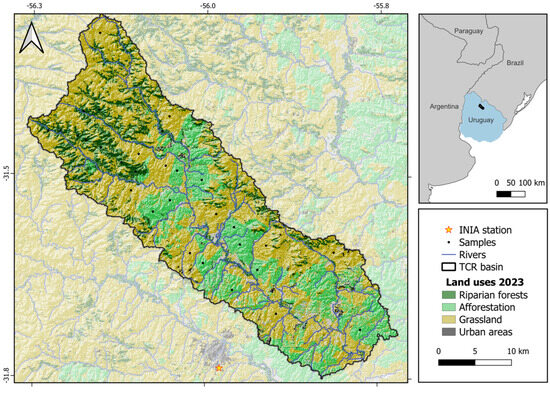
Figure 1.
Land use and land cover for the Tres Cruces River Basin for 2023.
The meteorological station is near the basin (~12 km), in the National Institute of Agricultural Research (INIA) of Tacuarembó (Figure 1); the proximity of the meteorological data station influenced the selection of this basin as the study area for this research. The climatological information from the INIA meteorological station shows an average annual precipitation of 1491.29 ± 379.00 mm from 1987 to 2024. The wettest year was 2002 (2797.30 mm), while the driest was 2004 (829.50 mm). The average annual evapotranspiration during the period was 1077.11 ± 64.55 mm. The highest estimated evapotranspiration was in 1989 (1232.80 mm), and the lowest was in 2001 (969.70 mm). The historical monthly data for precipitation from 1987 to 2024 indicate that monthly precipitation exceeds 80 mm in all months. Winter months are the driest, while spring and fall experience periods of wetness. The daily average temperature in winter is 14.09 ± 4.42, and in summer it is 21.53 ± 5.36 °C.
The Pampa biome covers Brazil, Uruguay, and Argentina, with a total area of 750,000 km2. The Pampa biome is a diverse ecological mosaic, seamlessly integrating grasslands, riparian forests, clusters of bushes, and slope forests into a single, dynamic landscape [13].
The TCR’s LULCC process has remained stable over the last decade (Figure 2), and the meteorological data station’s proximity influenced this basin’s selection as the study area for this research. As of 2023, afforestation occupies 216.9 km2 (23.6%), grassland 502.4 km2 (54.8%), and riparian forests 154.1 km2 (16.8%), according to the MapBiomas classification for 2015 and 2023 [23,24].
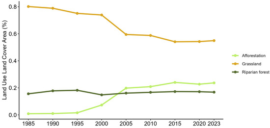
Figure 2.
Land use land cover change (1985 to 2023) based on MapBiomas data.
2.2. Standardized Precipitation-Evapotranspiration Index
The selected period for this study ranged from 2014 to 2024, incorporating the recent drought period (2020–2023), to analyze both drought-affected and non-drought-affected intervals. The Standardized Precipitation-Evapotranspiration Index (SPEI) was calculated using data from the INIA meteorological station. The SPEI calculation involves determining the difference between precipitation and evapotranspiration, estimated using the Penman–Monteith method [3].
The computational implementation of the SPEI was carried out using the SPEI package in R 4.4.2 [25]. This package provides an automated interface for calculation, integration with climatic time series data, and multiscale analysis. SPEI is a widely recognized tool for monitoring, analyzing, and detecting drought events. It assesses drought severity by combining precipitation and potential evapotranspiration data. It is especially useful for assessing the impact of climate change on droughts, as evapotranspiration is affected by temperature. The monthly difference between precipitation and potential evapotranspiration () was accumulated over a 12-month period. To standardize the SPEI, the accumulated values are fitted to a log-logistic statistical distribution, chosen for its effectiveness in modeling climatic extremes. Distribution parameters are estimated using probability-weighted moments, ensuring greater spatial and temporal consistency. After fitting the values, the data were transformed into a standardized scale with a mean of zero and a standard deviation of one. This transformation allows the SPEI to be consistently represented, making it easier to analyze and compare across different periods and locations [25,26].
2.3. Actual Evapotranspiration
The SAFER method, developed by Teixeira [8], is used to estimate actual evapotranspiration ( and has been extensively validated across various regions and climatic conditions. The model has demonstrated versatility and accuracy in various land uses, such as eucalyptus plantations, sugarcane, and pastures, showing its broad applicability [9,27,28,29,30,31,32,33].
The SAFER method was used to estimate actual evapotranspiration () and has been extensively validated across various regions and climatic conditions [9,29,33]. SAFER does not require the soil–water balance to estimate , as occurs in the SEBAL and METRIC methods, because it uses the energy balance to estimate . Developed by Teixeira [8], the algorithm is based on the relationship between reference evapotranspiration () and , expressed through the evapotranspiration fraction (), which is closer to the so-called crop coefficient (Kc) from FAO56.
where represents surface temperature in Kelvin, is surface albedo (dimensionless), NDVI is the Normalized Difference Vegetation Index (dimensionless), and and are empirically adjusted coefficients. Values for and were derived from Safre et al. [29] and Teixeira [8]. ETa is calculated by multiplying ETr and , as expressed by the following equation:
The implementation of SAFER relies on daily satellite imagery and meteorological data. For this purpose, we utilized images from Landsat 8 and 9 to derive NDVI, surface albedo, and temperature (using thermal bands) and meteorological data from INIA station, including global radiation (Rg) and reference evapotranspiration (), calculated using the Penman–Monteith method [3].
The NDVI is an indicator related to land cover, vegetation stages, and vegetation vigor [34], obtained from satellite imagery using the reflectance in the near-infrared (NIR) and red (RED) bands from Landsat. It is defined as follows:
Surface albedo was computed by first deriving planetary albedo ():
where is the spectral weight for each band, and is the associated reflectance. Weights were computed as the ratio of incoming shortwave radiation in a particular band to the total at the top of the atmosphere (TOA). The final surface albedo () was obtained through the following equation:
with c and d regression coefficients provided in the Agriwater package [9,34] as based on previous studies [8,28]. Temperatures were derived from Landsat band 10 and 11 spectral radiance ():
where are the pixel values of bands 10 and 11, and and are conversion coefficients available in the metadata of Landsat images.
The average value between and is corrected to retrieve the surface temperature by a regression curve:
where and are the regression coefficients, which for a 24 h period was considered as 1.11 and −31.89 and was calibrated with R2 = 0.95.
The SAFER model has been validated in multiple studies, for instance, in California vineyards [28], while studies in an ecological station in Brazil [30,31] reported similar accuracies. Additionally, Teixeira et al. [8,29] validated SAFER for semiarid regions in Brazil using orbital and aircraft images. The algorithm has been successfully applied to various land uses, such as eucalyptus plantations, sugarcane, and pastures, demonstrating its versatility.
2.3.1. Landsat Data
Imagery from Landsat 8 and Landsat 9 (Table 1) was used to derive key SAFER method parameters, including NDVI, surface albedo, and land surface temperature. Both satellites carry nearly identical sensors, the Operational Land Imager (OLI) and Thermal Infrared Sensor (TIRS) in Landsat 8, and the upgraded OLI-2 and TIRS-2 in Landsat 9, which provide consistent, quality data with a spatial resolution of 30 m for multispectral bands (15 m for the panchromatic band) and a temporal resolution of 16 days. When used together, these satellites offer an effective revisit rate of 8 days. Landsat 8, operational since 2013, and Landsat 9, launched in 2021, collectively ensure the continuity of data critical for numerous environmental and hydrological analyses.

Table 1.
Landsat 8 and 9 images used in the actual evapotranspiration calculation with SAFER.
All imagery was preprocessed in Google Earth Engine using the USGS Collection 2 Tier 1 TOA reflectance datasets (LANDSAT/LC08/C02/T1_TOA and LANDSAT/LC09/C02/T1_TOA). Preprocessing steps included calibrated reflectance of the top of the atmosphere (TOA), ensuring data consistency across temporal and spatial scales. Cloud masks were generated using the QA_PIXEL quality bands to exclude pixels affected by clouds, shadows, or other atmospheric disturbances, and subsequent filtering in R applied a 95% basin coverage threshold to ensure data quality for the interest area.
2.3.2. Data Processing
The data processing (Figure 3) was significantly simplified by utilizing the ‘agriwater’ R package. For each Landsat image (Table 1), the corresponding meteorological data were integrated to facilitate the execution of the package’s function. This function applies the set of equations and parameters presented in Section 2.3 to derive the ETa estimates; detailed information is provided in Silva et al. [9,34].
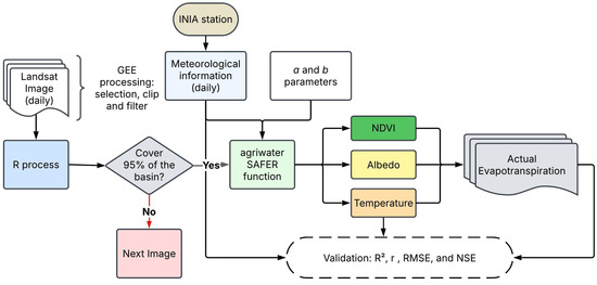
Figure 3.
Flowchart of the data processing.
To evaluate the quality of the estimates, four statistical metrics were employed: the Pearson correlation coefficient (r), the coefficient of determination (R2), the root-mean-square error (RMSE), and the Nash–Sutcliffe Efficiency (NSE). These metrics were calculated by comparing the estimated values of with the reference values recorded at the INIA meteorological station. Furthermore, the surface temperature () obtained from Landsat and the INIA station was also tested as an additional quality parameter. This approach utilized variables with low estimation complexity to assess potential uncertainties in the remote sensing-derived temperature information.
These indicators are widely used in hydrological and environmental modeling to assess the agreement between observed and estimated values. The Pearson correlation coefficient measures the strength and direction of the linear relationship between two variables, ranging from −1 to 1 [35]. The coefficient of determination quantifies the proportion of variance in the observed data explained by the model. It ranges from 0 to 1, and a high R2 suggests that the model effectively captures the variability in the observed data [36]. The root-mean-square error (RMSE) measures the average magnitude of the errors between observed and predicted values. It is expressed in the same units as the variable being analyzed and provides an absolute measure of the model’s predictive error [37]. The Nash–Sutcliffe Efficiency (NSE) is a normalized statistic that evaluates how well a model predicts observed values compared to the mean of the observations. NSE values range from −∞ to 1, where 1 indicates a perfect match between observed and estimated values, 0 implies that the model is only as good as using the mean of the observations, and negative values suggest that the model performs worse than the mean [38]. This metric is particularly useful for assessing hydrological models and time-series data.
3. Results
The SPEI from 1987 to 2024 (Figure 4) shows alternating cycles of drought and wet conditions. The index ranges from approximately −2 to +2, indicating a fluctuation between drought and wet without a clearly defined long-term trend. From 1987 to 1998, there was a rapid alternation between positive and negative values, suggesting pronounced climatic variability, highlighted by two significant drought periods: 1988–1991 and 1994–1998. In the period from 1998 to 2004, positive SPEI values prevailed, indicating a tendency toward wetter conditions. Conversely, from 2004 to 2014, there is a notable increase in the frequency of negative values, indicating a higher incidence of drought events. Finally, the period from 2014 to 2024 exhibits substantial variability, with alternating wet and dry years, including the last drought periods of 2020 and 2023.
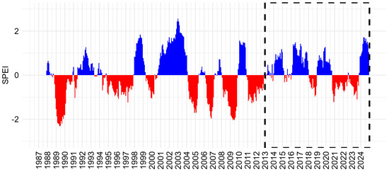
Figure 4.
Standardized Precipitation Evapotranspiration Index (SPEI) from 1987 to 2024; data from the INIA meteorological station. The dashed black lines represent the studied period from 2014 to 2024.
The implementation of SAFER in Uruguay proved successful, with parameters adjusted using sufficient literature data to estimate actual evapotranspiration (). The parameters a and b proposed by Safre et al. ([29], a = 0.66 and b = −0.0028) for vineyards in California performed exceptionally well. The selection of these parameter values was based on an evaluation of data quality compared with those presented by Teixeira ([8]; a = 1.8 and b = −0.008), which were the only alternatives available in the literature. To assess the data quality, several statistical indicators were computed using from meteorological stations and from images processed with SAFER (Figure 5c,d). For the Safre et al. [29] parameters, the results were R2 = 0.87, r = 0.94, RMSE = 1.46 mm day−1, and NSE = 0.34, while the evaluation using Teixeira [8] parameters produced R2 = 0.01, r = −0.11, RMSE = 2.90 mm day−1, and NSE = −1.62.
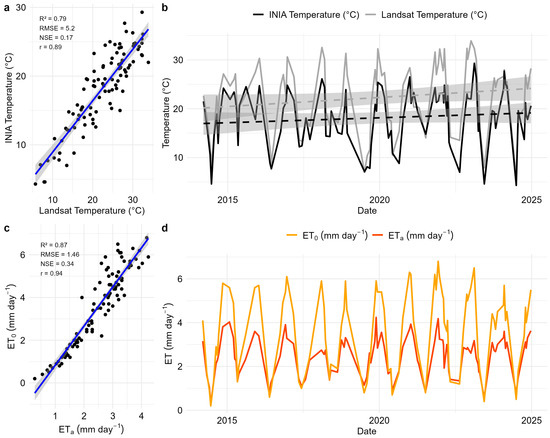
Figure 5.
(a,b) Surface temperature from Landsat and (c,d) actual evapotranspiration ( from SAFER estimation validation using temperature and potential evapotranspiration ( from INIA meteorological station data from 2014 to 2024.
The comparison between surface temperature data from the INIA meteorological station and Landsat (Figure 5a,b) reveals strong agreement, with R2 = 0.79, r = 0.89, RMSE = 5.2 °C, and NSE = 0.17. These results confirm the good accuracy of satellite data in relation to land-based measurements. Furthermore, the temporal analysis indicates an increasing trend in temperature from 2014 to 2024 in both datasets, with a more pronounced intensity observed in the Landsat data.
The seasonal trends in estimated by SAFER across afforestation, riparian forest, and grassland areas reflect the direct influence of climate variations, such as solar radiation, temperature, water availability, and plant physiological activity, on these ecosystems. Figure 6a presents the monthly variation in in the period from 2014 to 2024, clearly highlighting that all vegetation types reduce physiological activity during the cold months and increase it during the warm months. Afforestation areas exhibit the highest values throughout the year (with January values of 3.76 ± 0.48 mm day−1 and July values of 0.85 ± 0.33 mm day−1), followed by riparian forests (January = 3.70 ± 0.52 mm day−1 and July = 0.81 ± 0.31 mm day−1). Grasslands display the lowest values (January = 2.99 ± 0.66 mm day−1 and July = 0.74 ± 0.29 mm day−1), suggesting either a lower water demand or a reduced capacity to extract water from the soil.
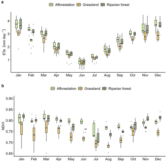
Figure 6.
Behavior of monthly actual evapotranspiration (a) and Normalized Difference Vegetation Index (b) from 2014 to 2024.
Complementary information on vegetation vigor is provided by the monthly normalized difference vegetation index (NDVI) shown in Figure 6b. The NDVI shows that riparian forests (January = 0.82 ± 0.01 and July = 0.72 ± 0.03) and grassland (January = 0.76 ± 0.05 and July = 0.68 ± 0.03) adapt to seasonal and hydrological characteristics, while the exotic vegetation used in afforestation maintains high vigor throughout the year (January = 0.81 ± 0.02 and July = 0.76 ± 0.04). NDVI values peak during the spring and summer months (October to March), indicating higher photosynthetic activity and increased plant biomass, and decline in autumn and winter (April to September). Notably, afforestation areas show the highest NDVI values, followed by riparian forests and then grasslands. This pattern reinforces the observation that exotic vegetation used in afforestation maintains high vigor throughout the year, associated with higher water consumption, as evidenced by its elevated . The alignment of seasonal NDVI and patterns suggest a direct relationship between photosynthetic activity, biomass accumulation, and water consumption across these land uses.
The temporal patterns of across different land uses in the TCR are presented in Figure 7. Two complementary analyses were performed to assess vegetation behavior and total water consumption. First, values were filtered for drought and wet years using SPEI data to compare vegetation behavior (Figure 7a). The results indicate that in afforestation areas, increased slightly during dry conditions (wet: 2.58 ± 1.07 mm day−1; dry: 2.67 ± 0.89 mm day−1). A similar pattern was observed in riparian forests (wet: 2.49 ± 1.06 mm day−1; dry: 2.59 ± 0.90 mm day−1), whereas grasslands showed a minor decrease in from wet (2.16 ± 0.90 mm day−1) to dry years (2.12 ± 0.70 mm day−1). These observations suggest that forested systems have a greater capacity to access water under restricted conditions compared to grasslands.
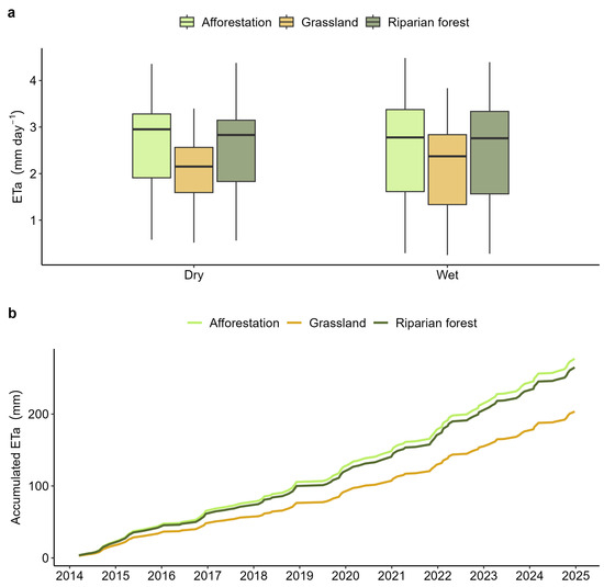
Figure 7.
Actual evapotranspiration for each land use during SPEI dry and wet periods (a) and accumulated actual evapotranspiration for samples of each land use ((b), see Figure 1) from 2014 to 2024.
Second, to gain a broader spatial and temporal perspective on total water consumption, daily values were accumulated. Since afforestation covers less than half the area of grassland, a hypothetical scenario assuming equal area coverage was examined by compiling accumulated values from 10 representative samples for each land use (Figure 1). The results reveal that, when normalized for the area, in afforestation is 26.50% higher than in grasslands and 4.79% higher than in riparian forests (Figure 7b).
The spatial and temporal dynamics of were analyzed using map-based visualizations, providing a clear representation of how different land uses respond to seasonal and interannual climate variations. In winter (Figure 8), values are generally lower due to reduced solar radiation, cooler temperatures, and diminished photosynthetic activity. In summer (Figure 9), afforestation areas stand out, with significantly higher compared to grasslands, while riparian forests also exhibit elevated levels, though slightly lower than in afforestation areas.
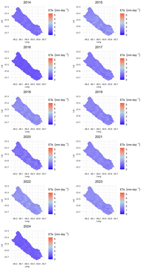
Figure 8.
Average actual evapotranspiration maps for winter months from 2014 to 2024.
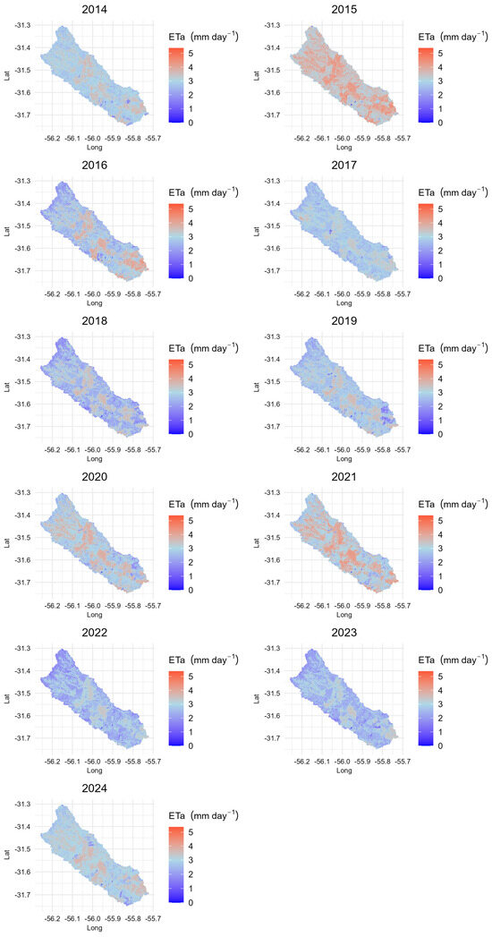
Figure 9.
Average actual evapotranspiration maps for summer months from 2014 to 2024.
Nevertheless, the spatial distribution still exhibits notable interannual variation, with some areas consistently showing higher or lower . Although the differences between dry and wet winters are less pronounced than those observed in summer, the maps indicate that drier winters tend to have a slightly higher than wetter winters.
4. Discussion
The effects of climate variability on water consumption and vegetation response, comparing natural vegetation (grasslands and riparian forests) and eucalyptus reforestation in the Tres Cruces River Basin (TCR), were verified by a major climate event during the study period, the prolonged drought of 2020–2023. Although the SPEI remained within the normal range (−1 to 1) during the broader period of 2014–2024, suggesting the absence of significant extremes of rainfall or drought throughout the decade, the prolonged duration of the 2020–2023 drought had notable consequences. Although not classified as “severe” in intensity according to SPEI, the prolonged duration of drought significantly impacted river flows [39], water quality [40,41], and agricultural activities [42], with repercussions also felt in Argentina [43]. Despite the limitations of the studied period in capturing the full extent of drought impact, the availability of Landsat imagery and the relative stability of LULCC during this decade provided optimal technical conditions for the evapotranspiration analysis (see Figure 2 and Table 1).
The performance of the SAFER method for estimating actual evapotranspiration () was assessed using several quality parameters. An r2 of 0.87 indicates that the model captures the variability in observed , while a Pearson correlation coefficient of 0.94 reflects a strong linear relationship between observed () and predicted values. An RMSE of 1.46 mm day−1 and an NSE of 0.34, although they may seem modest, are acceptable given the conceptual differences between the two evapotranspiration levels being compared. The average difference between grasslands and afforestation was 0.43 ± 0.32 mm day−1. According to Nosetto et al. [44], the same comparison ranged from approximately 0.6 to 2 mm day−1.
Potential evapotranspiration represents the maximum amount of water that could evaporate under ideal conditions, free from soil moisture restrictions. In contrast, actual evapotranspiration, calculated by the SAFER method, modifies this potential to reflect the specific water usage of each type of vegetation, considering factors such as water availability and plant physiology. This fundamental conceptual difference means that actual evapotranspiration will always be equal to or less than potential evapotranspiration. Consequently, when comparing these two estimates, it is natural to expect more variation in the data, leading to higher RMSE and lower NSE values. However, despite these differences, the obtained values allowed us to quantify the divergence between parameters a and b (Equation (1)), confirming that the model can accurately capture variations in water consumption due to different land uses.
The SAFER method, previously validated in California vineyards [28], has shown significant potential for reliable estimation. Its sensitivity to empirical coefficients requires local calibration to account for region-specific climatic conditions, a challenge that can be mitigated by integrating satellite imagery with regional meteorological data using tools such as the ‘agriwater’ package [9]. Although the lack of calibration data (e.g., from eddy covariance towers or lysimeters) may restrict its application in certain regions, the overall performance of SAFER in our study supports its utility in diverse environmental contexts. Validation with surface temperature and potential evapotranspiration (Figure 5) provides some assurance despite the limited data available for calibration.
Temporal analyses (Figure 6 and Figure 7) reveal that afforestation consistently exhibits the highest in both wet and dry conditions, while grasslands display the lowest values, and riparian forests occupy an intermediate position. This pattern suggests that tree-dominated systems, due to their greater biomass and higher photosynthetic activity, have a higher water demand compared to grasslands. The observed differences in are corroborated by NDVI measurements, which indicate increased vegetation vigor in afforested areas. The maps (Figure 8 and Figure 9) reveal substantial interannual variability in distribution, indicating that factors such as precipitation, temperature, and solar radiation strongly influence water consumption. Moreover, the maps distinguish between dry and wet years, with drier years displaying a higher proportion of warm-colored areas (indicative of elevated ) and wetter years showing comparatively lower values. Certain regions consistently present higher or lower , potentially reflecting geographical features (e.g., topography, proximity to water bodies), differences in vegetation species (e.g., eucalyptus versus pine), age of afforestation, or forest management practices.
These findings imply that conversion from pasture to afforestation could significantly alter the regional water balance, with important implications for water resource availability in the TCR basin. The higher evapotranspiration observed in afforested areas has broader hydrological implications. The maps reveal substantial interannual variability in distribution, indicating that factors such as precipitation, temperature, and solar radiation strongly influence water consumption. Moreover, the maps distinguish between dry and wet years, with dryer years displaying a higher proportion of warm-colored areas (indicative of elevated ) and wetter years showing comparatively lower values. Certain regions consistently present higher or lower , potentially reflecting geographical features (e.g., topography, proximity to water bodies), differences in vegetation species (e.g., eucalyptus versus pine), age of afforestation, or forest management practices.
Forested systems tend to reduce streamflow and alter groundwater dynamics, including increased infiltration and recharge and reduced groundwater storage [13,16,17,18,45,46]. In addition to the water footprint that the commercial afforestation process can cause, it is important to consider important biophysical processes, such as the modification of the energy balance or carbon fluxes in comparison to native species [47]. These changes raise critical sustainability concerns regarding the expansion of commercial forestry in Uruguay and underscore the need for integrated water resource management and land use planning.
Our findings highlight that even moderate but prolonged drought conditions can have significant hydrological impacts on afforested basins. The analyzed results (Figure 7a) indicate a slight increase in , which may suggest changes in Eucalyptus adaptation during periods of hydrological stress, a phenomenon that is not yet well understood [48,49]. The Eucalyptus exhibits adaptive capacity to drought stress by altering functional traits such as stomatal morphology, gas exchange parameters, and hydraulic conductance [47]. These changes can result in abnormal behavior in trees, which requires specific management in afforested areas [49].
The robust performance of the SAFER method in capturing dynamics, coupled with the observed differences in water consumption across various land uses, underscores the importance of considering both climatic variability and land cover changes in water resource management. These results provide valuable insights for policymakers and stakeholders, particularly in the context of ongoing commercial forestry expansion and its potential implications for regional hydrological cycles. The effect of climatic variability in forested areas needs to be further studied for appropriate management actions to solve environmental or economic demands [50].
Water resource management in afforested areas requires an integrated approach grounded in robust policies and strategic land-use planning [51,52]. It is essential to move beyond micro-scale assessments of hydrological impacts and adopt a river basin perspective to achieve a comprehensive understanding of forest–water interactions and their cumulative effects [52,53]. This broader view is crucial for anticipating and mitigating significant changes in the water regime that could affect multiple users and downstream ecosystems [52,54]. Implementing forest management practices that minimize water consumption by selected species, soil compaction and degradation, and sediment and nutrient transport to water bodies is essential [53]. Moreover, mounting pressure on water resources, exacerbated by global climate change, requires the forestry sector to adapt and actively contribute to the resilience of river basins [53,54]. Continuous hydrological monitoring, coupled with adaptive management, enables adjustments to practices and policies as new knowledge emerges and environmental conditions shift [51]. This approach must be collaborative and scientifically grounded to reconcile forest production with long-term water security.
5. Conclusions
Remote sensing-based methods for estimating actual evapotranspiration are efficient and accurate tools that enable comprehensive mapping and monitoring of this hydrological variable. The integration of satellite data with meteorological information is favorable to energy balance modeling using the SAFER method. Landsat 8 and 9 data provide another generation of medium-scale monitoring, enabling the use of SAFER as a tool for critical challenges in water resource management.
The use of SAFER in this study helps to understand how commercial afforestation can alter water consumption at the basin scale. It shows that increasing the area occupied by this exotic species reduces water content in other reservoirs of the hydrological cycle at the basin scale. The results obtained in the Tres Cruces River Basin demonstrate that land use change has a significant impact on evapotranspiration. Eucalyptus reforestation has been shown to have greater water demands than pastures and riparian forests. This is due to the specific characteristics of eucalyptus, such as its rapid growth, larger leaf area, and deep root system, which allows it to access greater volumes of water from the soil and subsoil. Consequently, this leads to a reduction in surface runoff, river streamflow, and groundwater.
This is especially significant considering the current economic plan and the imminent increase in forest production. In addition, the prolonged drought period from 2020 to 2023, although not severe in intensity, significantly impacted river flows, water quality, and agricultural activities. This period exhibited a slight increase in evapotranspiration in the forest vegetation. This highlights the need for continuous monitoring to provide data for water resource management, aiming to mitigate the effects of climate variability and land use changes on the hydrological process.
Although this research provides a valuable set of information and data on the impact of forestry activities on water resources, there is a need to expand efforts toward applications with higher spatial resolution and produce local calibration parameters. This highlights a research gap in developing specific monitoring networks for actual evapotranspiration, which would support the use of energy balance models (or others) in Uruguay. Such advances would increase the ability to interpret water consumption in different crops with greater accuracy, since evapotranspiration is a key variable and at the same time difficult to estimate accurately.
Author Contributions
L.V.S.: conceptualization, data organization and processing, analysis, methodology adaptation, investigation, data validation, and manuscript writing. C.d.O.F.S.: manuscript review and editing. A.H.: manuscript review and editing. C.S.Q.: manuscript review and editing. All authors have read and agreed to the published version of the manuscript.
Funding
C.S.Q. acknowledges the Coordination of Superior Level Staff Improvement (CAPES), for the grant under the process 88887.637660/21; and the São Paulo Research Foundation (FAPESP) for the grants under the processes 2022/14.849-7 and 2023/13.079-6.
Data Availability Statement
The meteorological data from INIA stations are available at https://www.inia.uy/gras/Clima, accessed on 17 April 2025. Satellite images from Landsat 8 and 9 can be accessed via Google Earth Engine (https://developers.google.com/earth-engine/datasets/catalog/landsat, accessed on 17 April 2025). The script utilized in this study was developed based on the functionalities provided by the Agriwater package (https://cran.r-project.org/package=agriwater, accessed on 17 April 2025).
Conflicts of Interest
The authors declare no conflicts of interest.
References
- Fisher, J.B.; Melton, F.; Middleton, E.; Hain, C.; Anderson, M.; Allen, R.; McCabe, M.F.; Hook, S.; Baldocchi, D.; Townsend, P.A.; et al. The Future of Evapotranspiration: Global Requirements for Ecosystem Functioning, Carbon and Climate Feedbacks, Agricultural Management, and Water Resources. Water Resour. Res. 2017, 53, 2618–2626. [Google Scholar] [CrossRef]
- Food of the United Nations (FAO). Remote Sensing Determination of Evapotranspiration: Algorithms, Strengths, Weaknesses, Uncertainty and Best Fit-for-Purpose; FAO: Cairo, Egypt, 2023. [Google Scholar]
- Allen, R.G.; Pereira, L.S.; Raes, D.; Smith, M. Crop Evapotranspiration-Guidelines for Computing Crop Water Requirements; FAO Irrigation and Drainage Paper 56; FAO—Food and Agriculture Organization of the United Nations: Rome, Italy, 1998. [Google Scholar]
- Baldocchi, D.; Falge, E.; Gu, L.; Olson, R.; Hollinger, D.; Running, S.; Anthoni, P.; Bernhofer, C.; Davis, K.; Evans, R.; et al. FLUXNET: A New Tool to Study the Temporal and Spatial Variability of Ecosystem-Scale Carbon Dioxide, Water Vapor, and Energy Flux Densities. Bull. Am. Meteorol. Soc. 2001, 82, 2415–2437. [Google Scholar] [CrossRef]
- Fuentes, I.; Vervoort, R.W.; McPhee, J. Global Evapotranspiration Models and Their Performance at Different Spatial Scales: Contrasting a Latitudinal Gradient against Global Catchments. J. Hydrol. 2024, 628, 130477. [Google Scholar] [CrossRef]
- Bastiaanssen, W.G.M.; Menenti, M.; Feddes, R.A.; Holtslag, A.A.M. A Remote Sensing Surface Energy Balance Algorithm for Land (SEBAL). 1. Formulation. J. Hydrol. 1998, 212–213, 198–212. [Google Scholar] [CrossRef]
- Allen, R.G.; Tasumi, M.; Morse, A.; Trezza, R.; Wright, J.L.; Bastiaanssen, W.; Kramber, W.; Lorite, I.; Robison, C.W. Satellite-Based Energy Balance for Mapping Evapotranspiration with Internalized Calibration (METRIC)—Applications. J. Irrig. Drain. Eng. 2007, 133, 395–406. [Google Scholar] [CrossRef]
- Teixeira, A. Determining Regional Actual Evapotranspiration of Irrigated Crops and Natural Vegetation in the São Francisco River Basin (Brazil) Using Remote Sensing and Penman-Monteith Equation. Remote Sens. 2010, 2, 1287–1319. [Google Scholar] [CrossRef]
- Silva, C.O.F.; Teixeira, A.H.d.C.; Manzione, R.L. Agriwater: An R Package for Spatial Modelling of Energy Balance and Actual Evapotranspiration Using Satellite Images and Agrometeorological Data. Environ. Model. Softw. 2019, 120, 104497. [Google Scholar] [CrossRef]
- Barboza, N.; Laguna, H.; Mila, F. Apoyos y Gravámenes En La Actividad Forestal. In Anuario OPYPA 2021; MGAP: Montevideo, Uruguay, 2021; Available online: https://www.gub.uy/ministerio-ganaderia-agricultura-pesca/comunicacion/publicaciones/anuario-opypa-2021/estudios/apoyos-gravamenes-actividad-forestal-1 (accessed on 17 April 2025).
- Olmos, V.M.; Pienika, E. Contribution of the Forest Sector to the Uruguayan Economy: A First Approach with National Accounts. J. Sci. 2022, 68, 116–119. [Google Scholar] [CrossRef]
- DGF Dirección General Forestal; MGAP Ministerio de Ganadería Agricultura y Pesca. Resultados Cartografía Forestal; MGAP: Montevideo, Uruguay, 2021; Available online: https://www.gub.uy/ministerio-ganaderia-agricultura-pesca/comunicacion/noticias/nueva-cartografia-forestal-2021 (accessed on 17 April 2025).
- Reichert, J.M.; Rodrigues, M.F.; Peláez, J.J.Z.; Lanza, R.; Minella, J.P.G.; Arnold, J.G.; Cavalcante, R.B.L. Water Balance in Paired Watersheds with Eucalyptus and Degraded Grassland in Pampa Biome. Agric. For. Meteorol. 2017, 237–238, 282–295. [Google Scholar] [CrossRef]
- Ebling, É.D.; Reichert, J.M.; Zuluaga Peláez, J.J.; Rodrigues, M.F.; Valente, M.L.; Lopes Cavalcante, R.B.; Reggiani, P.; Srinivasan, R. Event-Based Hydrology and Sedimentation in Paired Watersheds under Commercial Eucalyptus and Grasslands in the Brazilian Pampa Biome. Int. Soil. Water Conserv. Res. 2021, 9, 180–194. [Google Scholar] [CrossRef]
- Jorge, B.C.S.; Winck, B.R.; da Silva Menezes, L.; Bellini, B.C.; Pillar, V.D.; Podgaiski, L.R. Grassland Afforestation with Eucalyptus Affect Collembola Communities and Soil Functions in Southern Brazil. Biodivers. Conserv. 2022, 32, 275–295. [Google Scholar] [CrossRef]
- Alonso, J.; Silveira, L.; Vervoort, R.W. Assessing Effects of Afforestation on Streamflow in Uruguay: From Small to Large Basins. Hydrol. Process 2024, 38, e15272. [Google Scholar] [CrossRef]
- Silveira, L.; Gamazo, P.; Alonso, J.; Martínez, L. Effects of Afforestation on Groundwater Recharge and Water Budgets in the Western Region of Uruguay. Hydrol. Process 2016, 30, 3596–3608. [Google Scholar] [CrossRef]
- Cano, D.; Cacciuttolo, C.; Custodio, M.; Nosetto, M. Effects of Grassland Afforestation on Water Yield in Basins of Uruguay: A Spatio-Temporal Analysis of Historical Trends Using Remote Sensing and Field Measurements. Land 2023, 12, 185. [Google Scholar] [CrossRef]
- Mer, F.; Vervoort, R.W.; Baethgen, W. Building Trust in SWAT Model Scenarios through a Multi-Institutional Approach in Uruguay. Socio-Environ. Syst. Model. 2020, 2, 17892. [Google Scholar] [CrossRef]
- Hoogar, R.; Malakannavar, S.; Hoogar, C.R.; Sujatha, H. Impact of Eucalyptus Plantations on Ground Water and Soil Ecosystem in Dry Regions. J. Pharmacogn. Phytochem. 2019, 8, 2929. [Google Scholar]
- Gallego, F.; Camba Sans, G.; Di Bella, C.M.; Tiscornia, G.; Paruelo, J.M. Performance of Real Evapotranspiration Products and Water Yield Estimations in Uruguay. Remote Sens. Appl. 2023, 32, 101043. [Google Scholar] [CrossRef]
- Navas, R.; Tiscornia, G.; Berger, A.G.; Otero, A. Evaluación de La Evapotranspiración de MODIS16A2 En Tres Resoluciones Espaciales En Uruguay. Agrociencia Urug. 2021, 25, 429. [Google Scholar] [CrossRef]
- Baeza, S.; Vélez-Martin, E.; De Abelleyra, D.; Banchero, S.; Gallego, F.; Schirmbeck, J.; Veron, S.; Vallejos, M.; Weber, E.; Oyarzabal, M.; et al. Two Decades of Land Cover Mapping in the Río de La Plata Grassland Region: The MapBiomas Pampa Initiative. Remote Sens. Appl. 2022, 28, 100834. [Google Scholar] [CrossRef]
- MapBiomas. Pampa Trinacional: Argentina, Brasil y Uruguay (Colección 3). 2023. Available online: https://pampa.mapbiomas.org/pt/home-3/ (accessed on 17 April 2025).
- Vicente-Serrano, S.M.; Beguería, S.; López-Moreno, J.I. A Multiscalar Drought Index Sensitive to Global Warming: The Standardized Precipitation Evapotranspiration Index. J. Clim. 2010, 23, 1696–1718. [Google Scholar] [CrossRef]
- Beguería, S.; Vicente-Serrano, S.M.; Reig, F.; Latorre, B. Standardized Precipitation Evapotranspiration Index (SPEI) Revisited: Parameter Fitting, Evapotranspiration Models, Tools, Datasets and Drought Monitoring. Int. J. Climatol. 2014, 34, 3001–3023. [Google Scholar] [CrossRef]
- Teixeira, A.H.d.C.; Hernandez, F.B.T.; Andrade, R.G.; Leivas, J.F.; Bolfe, E.L. Energy Balance with Landsat Images in Irrigated Central Pivots with Corn Crop in the São Paulo State, Brazil. In Proceedings of the SPIE—The International Society for Optical Engineering, San Diego, CA, USA, 17–21 August 2014; Volume 9239, pp. 219–228. [Google Scholar] [CrossRef]
- Safre, A.L.S.; Nassar, A.; Torres-Rua, A.; Aboutalebi, M.; Saad, J.C.C.; Manzione, R.L.; de Castro Teixeira, A.H.; Prueger, J.H.; McKee, L.G.; Alfieri, J.G.; et al. Performance of Sentinel-2 SAFER ET Model for Daily and Seasonal Estimation of Grapevine Water Consumption. Irrig. Sci. 2022, 40, 635–654. [Google Scholar] [CrossRef]
- Teixeira, A.; Pacheco, E.; Silva, C.; Dompieri, M.; Leivas, J. SAFER Applications for Water Productivity Assessments with Aerial Camera Onboard a Remotely Piloted Aircraft (RPA). A Rainfed Corn Study in Northeast Brazil. Remote Sens. Appl. 2021, 22, 100507. [Google Scholar] [CrossRef]
- Silva, C.O.F.; Manzione, R.L.; Albuquerque Filho, J.L. Large-Scale Spatial Modeling of Crop Coefficient and Biomass Production in Agroecosystems in Southeast Brazil. Horticulturae 2018, 4, 33. [Google Scholar] [CrossRef]
- Silva, C.O.F.; Manzione, R.L.; Albuquerque Filho, J.L. Combining Remotely Sensed Actual Evapotranspiration and GIS Analysis for Groundwater Level Modeling. Environ. Earth Sci. 2019, 78, 462. [Google Scholar] [CrossRef]
- Wagner Wolff Francisco, J.P.; Flumignan, D.L.; Marin, F.R.; Folegatti, M. V Optimized Algorithm for Evapotranspiration Retrieval via Remote Sensing. Agric. Water Manag. 2022, 262, 107390. [Google Scholar] [CrossRef]
- Rouse, J.; Haas, R.; Schell, J. Monitoring Vegetation Systems in the Great Plains with ERTS; NASA: Greenbelt, MD, USA, 1974. [Google Scholar]
- Silva, C.O.F.; Teixeira, A.H.D.C.; Manzione, R.L. Agriwater: Evapotranspiration and Energy Fluxes Spatial Analysis. CRAN: Contributed Packages, 2023. [Google Scholar] [CrossRef]
- Rodgers, J.L.; Nicewander, W.A. Thirteen Ways to Look at the Correlation Coefficient. Am. Stat. 1988, 42, 59–66. [Google Scholar] [CrossRef]
- Willmott, C.J. On the Validation of Models. Phys. Geogr. 1981, 2, 184–194. [Google Scholar] [CrossRef]
- Chai, T.; Draxler, R.R. Root Mean Square Error (RMSE) or Mean Absolute Error (MAE)?—Arguments against Avoiding RMSE in the Literature. Geosci. Model. Dev. 2014, 7, 1247–1250. [Google Scholar] [CrossRef]
- Nash, J.E.; Sutcliffe, J. V River Flow Forecasting through Conceptual Models Part I—A Discussion of Principles. J. Hydrol. 1970, 10, 282–290. [Google Scholar] [CrossRef]
- Cataldo, D.; Bordet, F.; Bruno, L. Efecto de La Bajante Extrema 2020-2023 Sobre La Reproducción de Peces Migradores En El Río Uruguay. Innotec 2024, 27, e653. [Google Scholar] [CrossRef] [PubMed]
- Nion, C.F.; Isasa, I.D. Spatial Distribution of Pesticide Use Based on Crop Rotation Data in La Plata River Basin: A Case Study from an Agricultural Region of Uruguay. Environ. Monit. Assess. 2024, 196, 633. [Google Scholar] [CrossRef]
- Rodríguez-Gallego, L.; Lescano, C.; Pasquariello, S.; Rodó, E.; Cardoso, A.; Serra, S.; Martínez, A.; Costa, S.; Nin, M.; Fernández, A. Proliferación de Plantas Sumergidas En La Laguna Garzón: Causas, Consecuencias y Recomendaciones de Manejo. Innotec 2024, 28, e655. [Google Scholar]
- Giuliano, F.; Navia, D.; Ruberl, H. The Macroeconomic Impact of Climate Shocks in Uruguay; World Bank: Washington, DC, USA, 2024. [Google Scholar]
- Conte, A.S. La Sequía 2020-2023 en la Argentina y su Impacto en la Agricultura; Consejo Nacional de Investigaciones Científicas y Técnicas: Buenos Aires, Argentina, 2024. [Google Scholar]
- Nosetto, M.D.; Jobbágy, E.G.; Paruelo, J.M. Land-Use Change and Water Losses: The Case of Grassland Afforestation across a Soil Textural Gradient in Central Argentina. Glob. Change Biol. 2005, 11, 1101–1117. [Google Scholar] [CrossRef]
- Silveira, L.; Alonso, J. Runoff Modifications Due to the Conversion of Natural Grasslands to Forests in a Large Basin in Uruguay. Hydrol. Process 2009, 23, 320–329. [Google Scholar] [CrossRef]
- Dresel, P.E.; Dean, J.F.; Perveen, F.; Webb, J.A.; Hekmeijer, P.; Adelana, S.M.; Daly, E. Effect of Eucalyptus Plantations, Geology, and Precipitation Variability on Water Resources in Upland Intermittent Catchments. J. Hydrol. 2018, 564, 723–739. [Google Scholar] [CrossRef]
- Dieguez, H.; Piñeiro, G.; Paruelo, J. Unraveling Impacts on Carbon, Water and Energy Exchange of Pinus Plantations in South American Temperate Ecosystems. Sci. Total Environ. 2024, 953, 176150. [Google Scholar] [CrossRef] [PubMed]
- Yang, L.; Kong, J.; Gao, Y.; Chen, Z.; Lin, Y.; Zeng, S.; Su, Y.; Li, J.; He, Q.; Qiu, Q. A Simulated Drier Climate Reduces Growth and Alters Functional Traits of Eucalyptus Trees: A Three-Year Experiment in South China. For. Ecol. Manag. 2023, 549, 121435. [Google Scholar] [CrossRef]
- Tupinambá-Simões, F.; Bravo, F.; Guerra-Hernández, J.; Pascual, A. Assessment of Drought Effects on Survival and Growth Dynamics in Eucalypt Commercial Forestry Using Remote Sensing Photogrammetry. A Showcase in Mato Grosso, Brazil. For. Ecol. Manag. 2022, 505, 119930. [Google Scholar] [CrossRef]
- Keenan, R.J. Climate Change Impacts and Adaptation in Forest Management: A Review. Ann. For. Sci. 2015, 72, 145–167. [Google Scholar] [CrossRef]
- FAO. Voluntary Guidelines on the Responsible Governance of Tenure of Land, Fisheries and Forests in the Context of National Food Security; Revised; FAO: Rome, Italy, 2022. [Google Scholar]
- Haas, H.; Kalin, L.; Sun, G.; Kumar, S. Understanding the Effects of Afforestation on Water Quantity and Quality at Watershed Scale by Considering the Influences of Tree Species and Local Moisture Recycling. J. Hydrol. 2024, 640, 131739. [Google Scholar] [CrossRef]
- Buechel, M.; Slater, L.; Dadson, S. Broadleaf Afforestation Impacts on Terrestrial Hydrology Insignificant Compared to Climate Change in Great Britain. Hydrol. Earth Syst. Sci. 2024, 28, 2081–2105. [Google Scholar] [CrossRef]
- Farooqi, T.J.A.; Portela, R.; Xu, Z.; Pan, S.; Irfan, M.; Ali, A. Advancing Forest Hydrological Research: Exploring Global Research Trends and Future Directions through Scientometric Analysis. J. Res. 2024, 35, 128. [Google Scholar] [CrossRef]
Disclaimer/Publisher’s Note: The statements, opinions and data contained in all publications are solely those of the individual author(s) and contributor(s) and not of MDPI and/or the editor(s). MDPI and/or the editor(s) disclaim responsibility for any injury to people or property resulting from any ideas, methods, instructions or products referred to in the content. |
© 2025 by the authors. Licensee MDPI, Basel, Switzerland. This article is an open access article distributed under the terms and conditions of the Creative Commons Attribution (CC BY) license (https://creativecommons.org/licenses/by/4.0/).