

Multivariate Statistical Modeling of Seasonal River Water Quality Using Limited Hydrological and Climatic Data

Abstract
:1. Introduction
2. Materials and Methods
2.1. Kiso River
2.2. Water Quality Parameters
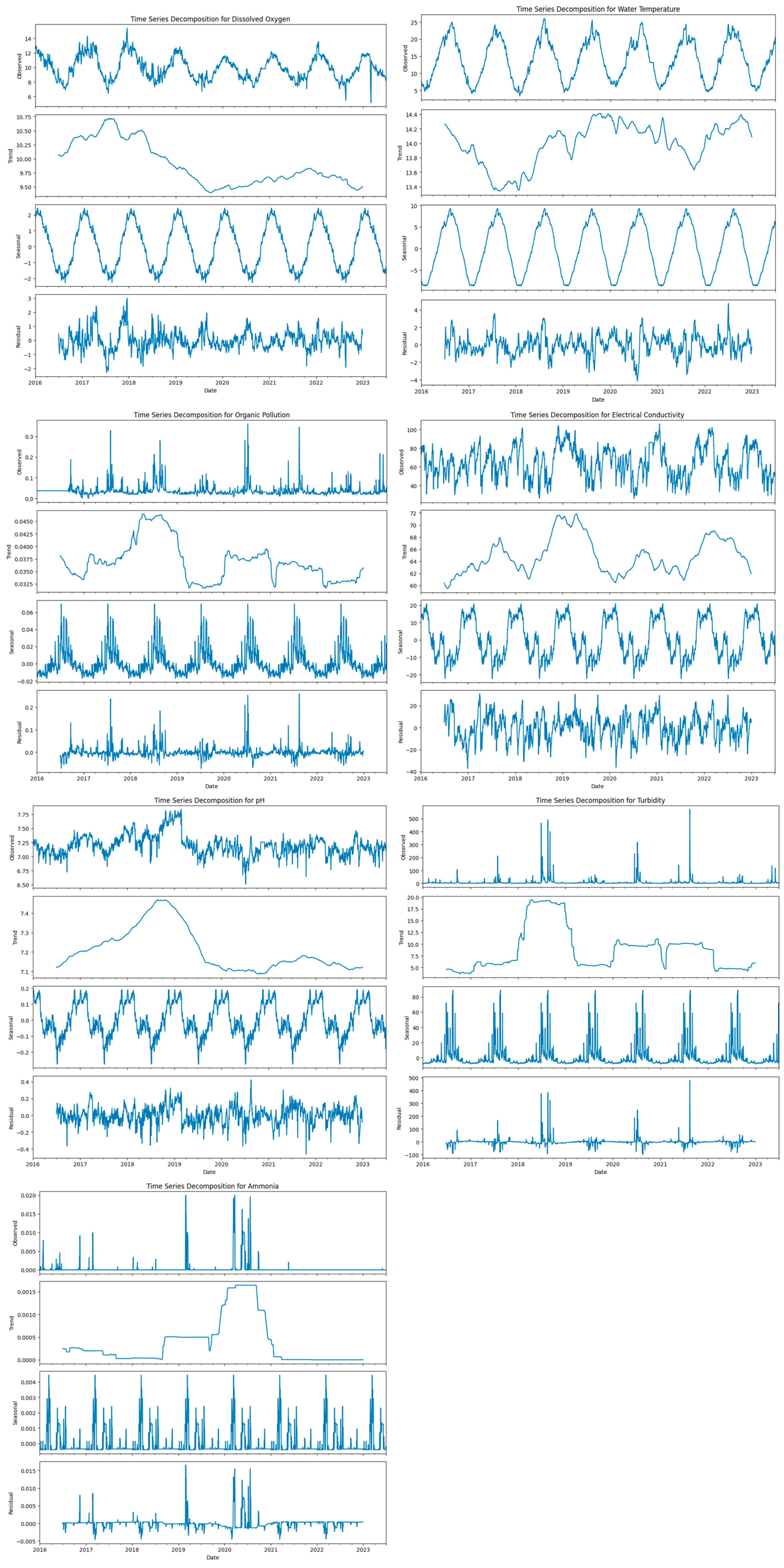
Time Series Decomposition
2.3. Seasonal Variation of Hydrological and Climatic Data
2.3.1. Seasonal Variation in River Flow
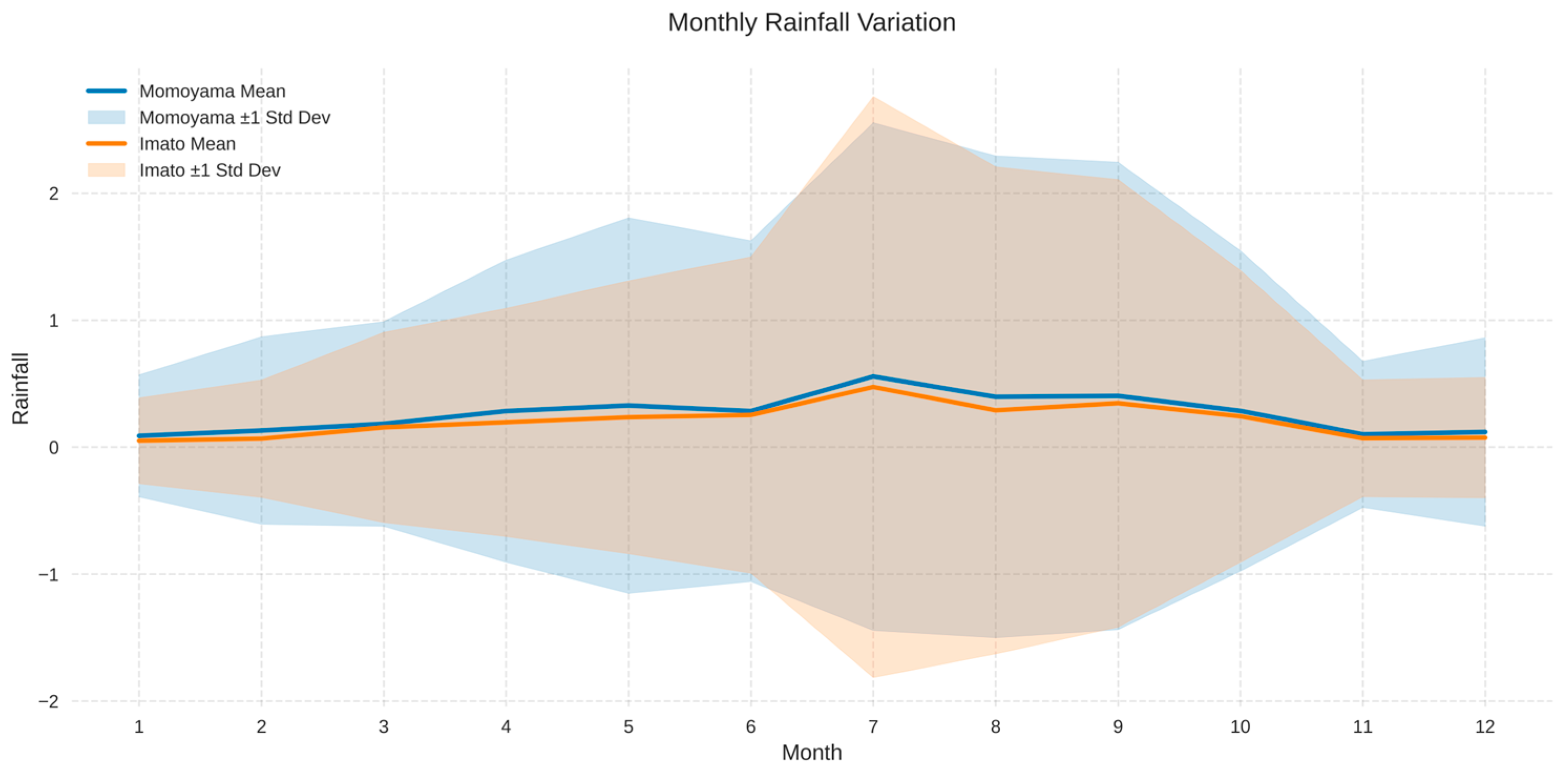
2.3.2. Seasonal Variation in Rainfall
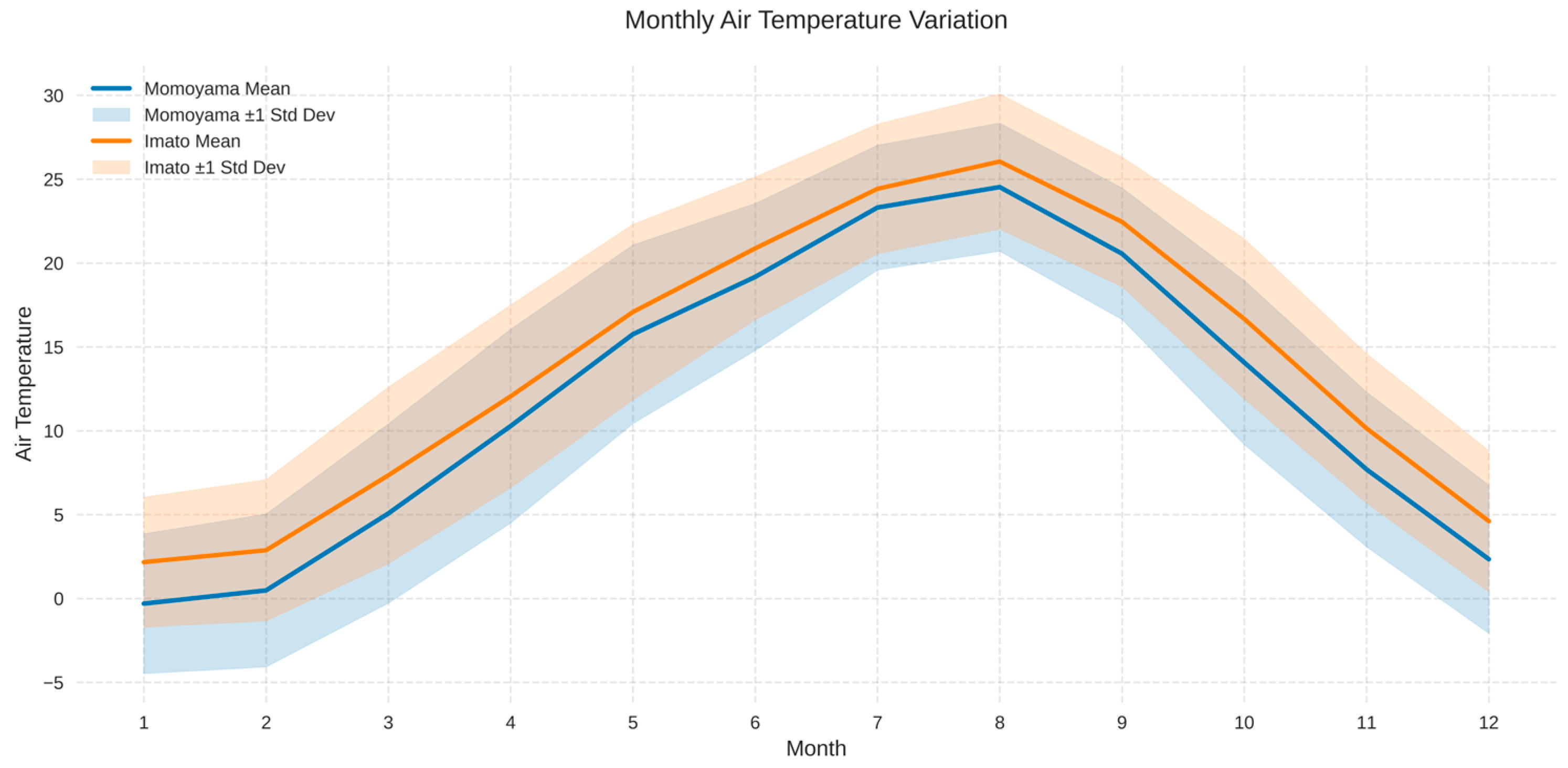
2.3.3. Seasonal Variation in Air Temperature
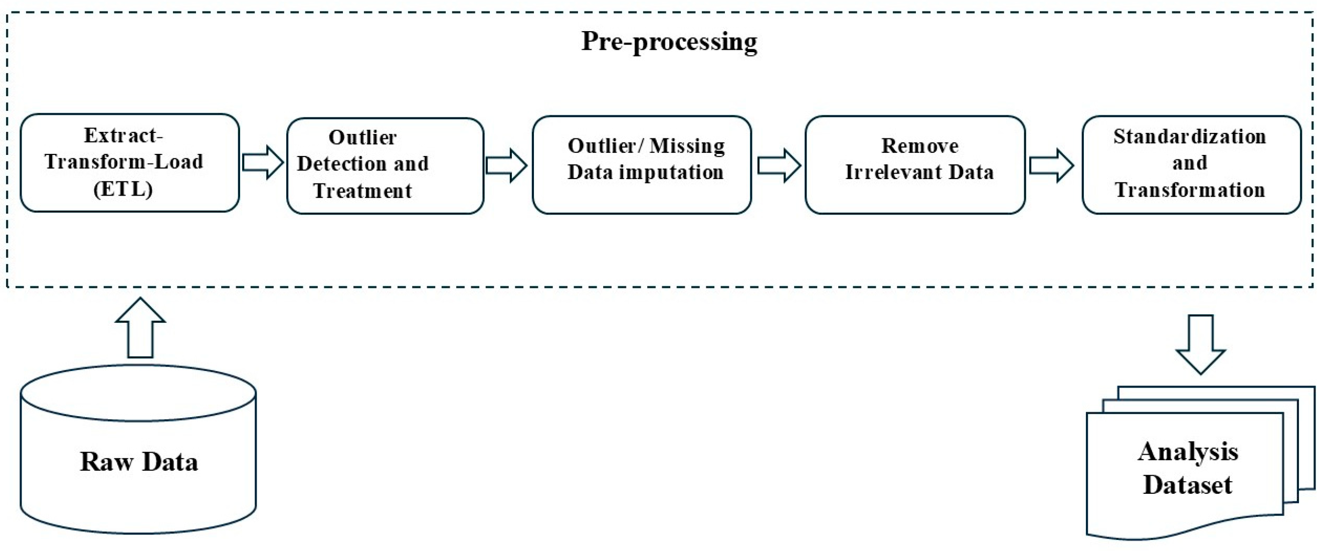
2.4. Pre-Processing of Data
2.5. Statistical Analysis
2.5.1. Descriptive Statistics
2.5.2. Correlation Analysis
2.5.3. Generalized Additive Model (GAM)
- is the dependent variable;
- β is recognized as any strictly parametric component;
- are smooth function notations;
- εi is a normal random variable.
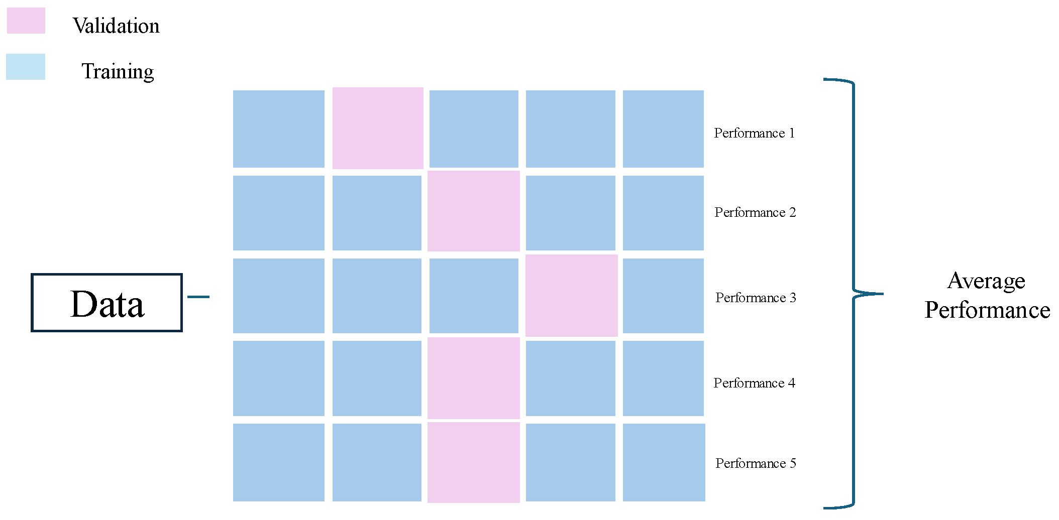
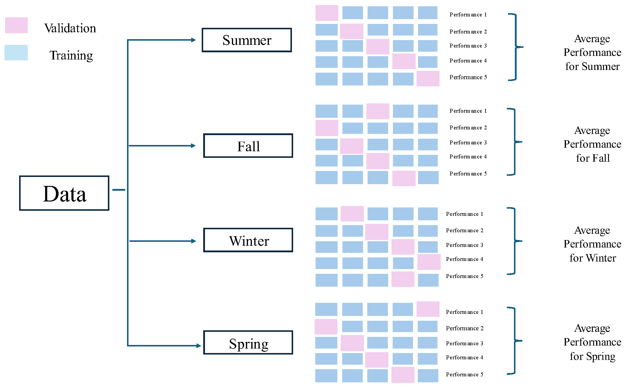
2.5.4. Model Validation
2.5.5. Evaluation Metrics
- = predicted value of ;
- = mean value of
3. Results and Discussion
3.1. Statistical Summary of Water Quality Parameters
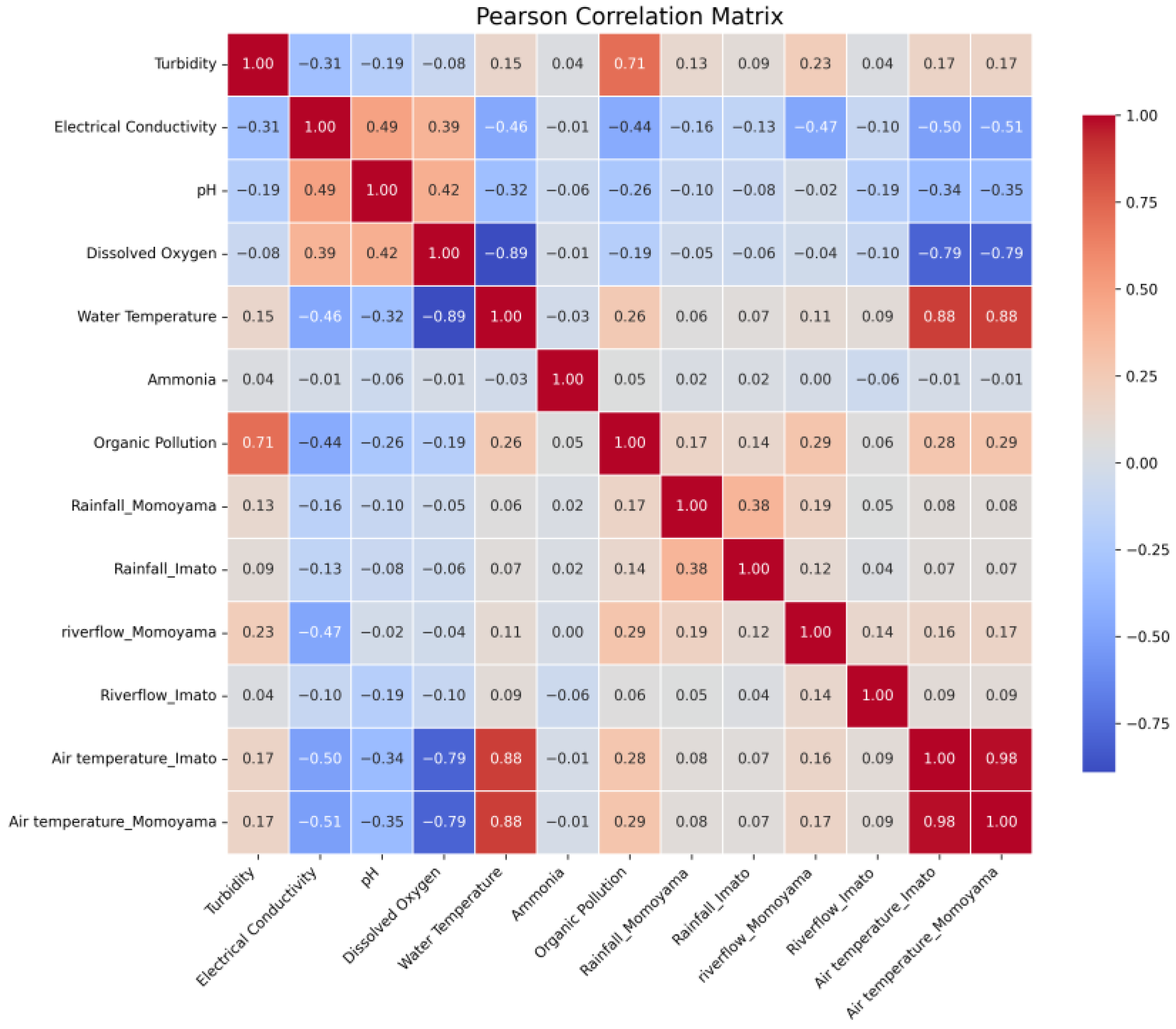
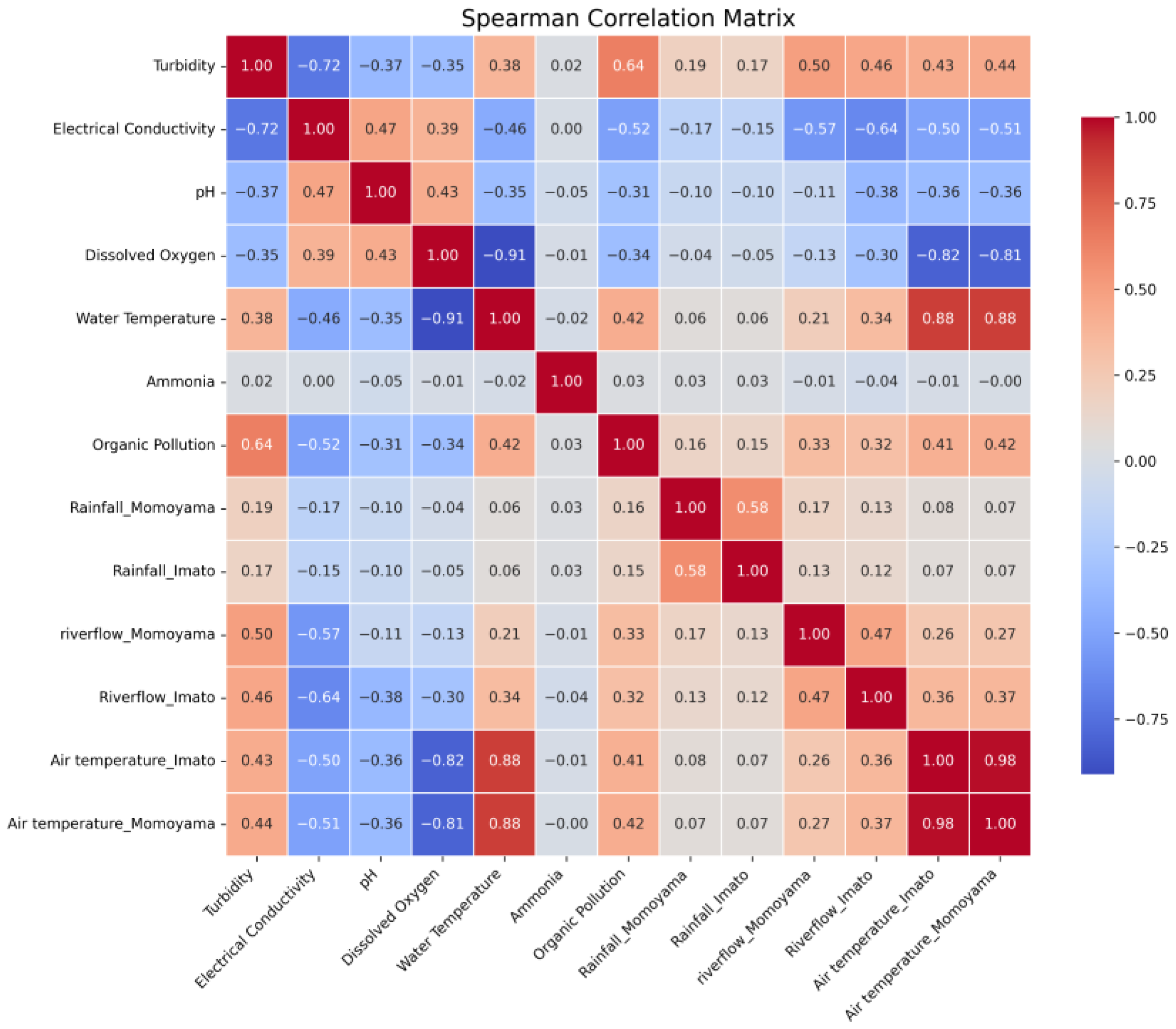
3.2. Correlation Analysis Results
3.3. General Additive Model (GAM)
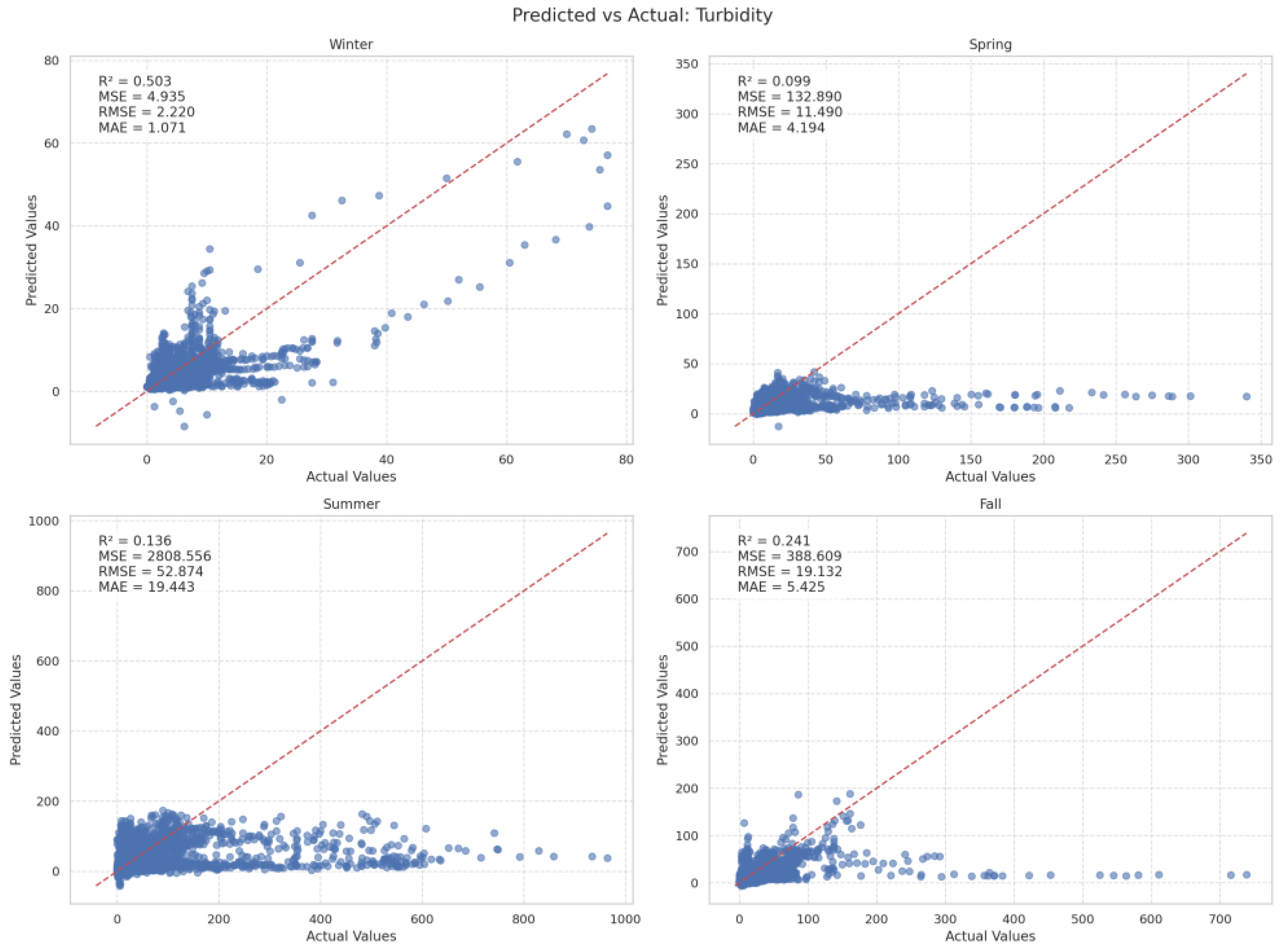
3.3.1. Turbidity
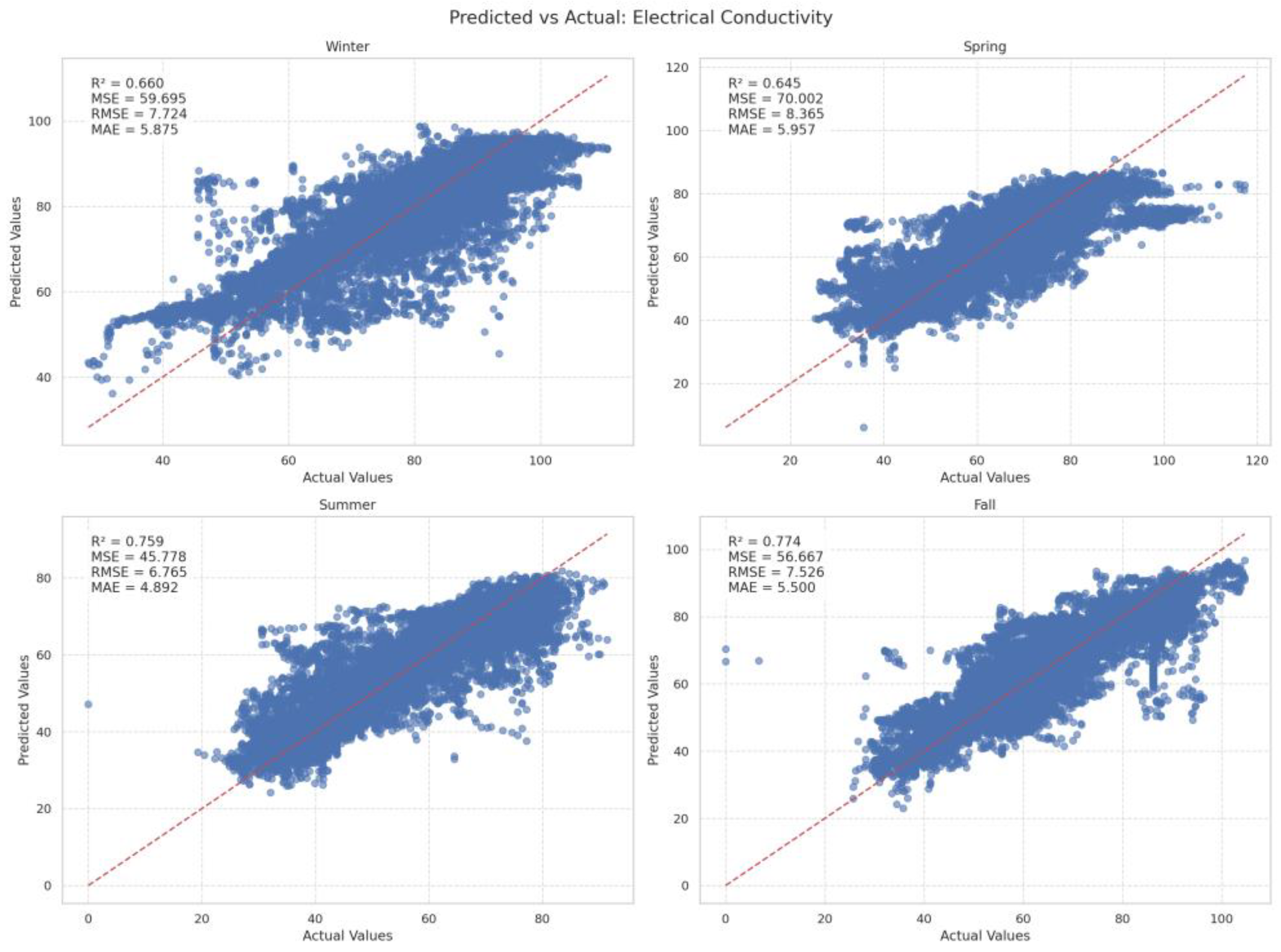
3.3.2. Electrical Conductivity (EC)
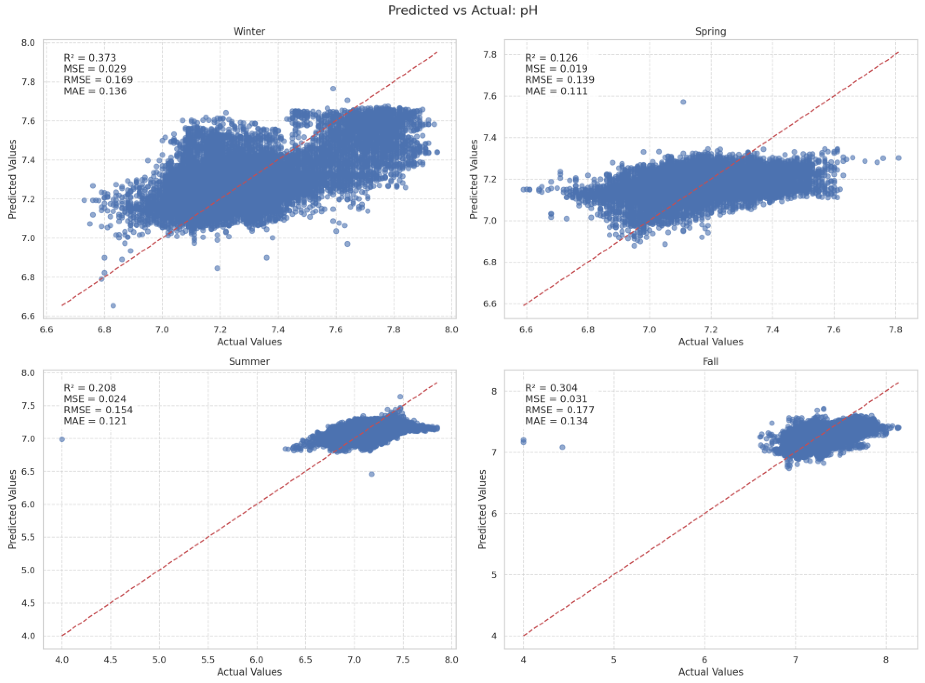
3.3.3. pH and Dissolved Oxygen (DO)
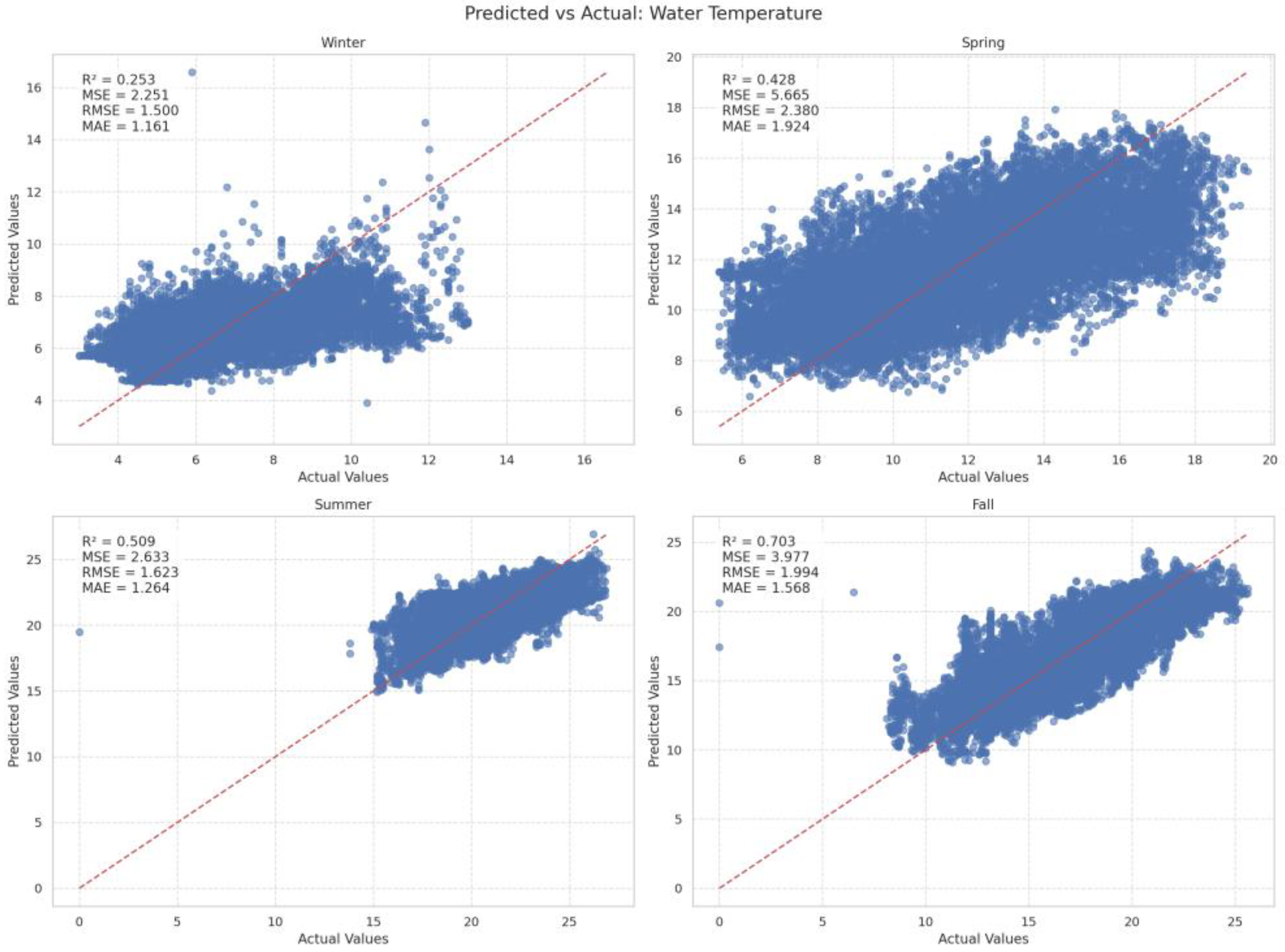
3.3.4. Water Temperature
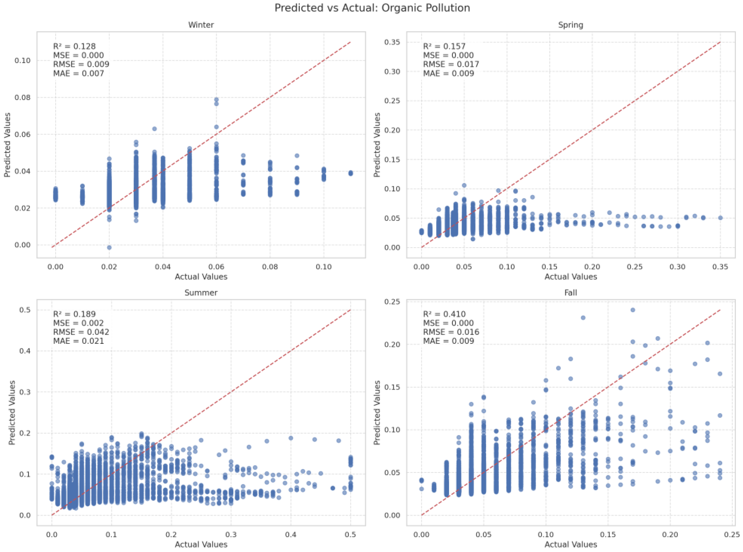
3.3.5. Ammonia and Organic Pollution
4. Conclusions
Author Contributions
Funding
Data Availability Statement
Acknowledgments
Conflicts of Interest
References
- Ding, J. Factors Affecting Water Quality in the Liao River Basin. In Highlights in Science, Engeneering and Tehnology; Darcy & Roy Press: Hillsboro, OR, USA, 2024; Volume 2023. [Google Scholar]
- Mamun, M.; Kim, J.Y.; Kim, J.E.; An, K.G. Longitudinal Chemical Gradients and the Functional Responses of Nutrients, Organic Matter, and Other Parameters to the Land Use Pattern and Monsoon Intensity. Water 2022, 14, 237. [Google Scholar] [CrossRef]
- Bessa Santos, R.M.; Farias do Valle, R., Jr.; Abreu Pires de Melo Silva, M.M.; Tarlé Pissarra, T.C.; Carvalho de Melo, M.; Valera, C.A.; Leal Pacheco, F.A.; Sanches Fernandes, L.F. A framework model to integrate sources and pathways in the assessment of river water pollution. Environ. Pollut. 2024, 347, 123661. [Google Scholar] [CrossRef] [PubMed]
- Surendra, P.; Saurabh, A.H. Impact Analysis of Urbanization and Industrialization on Water Quality of Vrishabhavathi River. Geogr. Anal. 2021, 10, 45–51. [Google Scholar] [CrossRef]
- Anh, N.T.; Can, L.D.; Nhan, N.T.; Schmalz, B.; Luu, T.L. Influences of key factors on river water quality in urban and rural areas: A review. Case Stud. Chem. Environ. Eng. 2023, 8, 100424. [Google Scholar] [CrossRef]
- Sani, Z.; Tshimanga, R.M.; Odume, O.N.; Basamba, T.A.; Katshiatshia, H.M. Developing an approach for balancing water use and protecting water quality of an urban river ecosystem. Phys. Chem. Earth 2024, 136, 103687. [Google Scholar] [CrossRef]
- Laura, K.S.H. Surface Water Quality Changes of River Reaches Due to Urbanization. In Proceedings of the in Water Resources and Wetlands Conference, Tulcea, Romania, 14–16 September 2012; Transversal: Viena, Austria, 2012. [Google Scholar]
- Quadir, A. Urbanization and its Impact on Ganga Basin. Int. J. Sci. Res. Publ 2022, 12, 371. [Google Scholar] [CrossRef]
- Wu, J.; Qin, C.X.; Yue, Y.; Cheng, S.P.; Zeng, H.; He, L.Y. Comprehensive effects of climate, land use/cover and management practices on runoff and nutrient variations in a rapidly urbanizing watershed. Chemosphere 2024, 349, 140934. [Google Scholar] [CrossRef]
- Schaffer-Smith, D.; DeMeester, J.E.; Tong, D.; Myint, S.W.; Libera, D.A.; Muenich, R.L. Landscape Pollution Source Dynamics Highlight Priority Locations for Basin-Scale Interventions to Protect Water Quality Under Hydroclimatic Variability. Earths Future 2023, 11, e2022EF003137. [Google Scholar] [CrossRef]
- Tong, S.T.Y.; Liu, A.J.; Goodrich, J.A. Climate Change Impacts on Nutrient and Sediment Loads in a Midwestern Agricultural Watershed. J. Environ. Inform. 2007, 9, 18–28. [Google Scholar] [CrossRef]
- Ducharne, A. Hydrology and Earth System Sciences Importance of stream temperature to climate change impact on water quality. Hydrol. Earth Syst. Sci. 2008, 12, 797–810. [Google Scholar] [CrossRef]
- Ficklin, D.L.; Stewart, I.T.; Maurer, E.P. Effects of climate change on stream temperature, dissolved oxygen, and sediment concentration in the Sierra Nevada in California. Water. Resour. Res. 2013, 49, 2765–2782. [Google Scholar] [CrossRef]
- Rajesh, M.; Rehana, S. Impact of climate change on river water temperature and dissolved oxygen: Indian riverine thermal regimes. Sci. Rep. 2022, 12, 9222. [Google Scholar] [CrossRef] [PubMed]
- Morrill, J.C.; Bales, R.C.; Conklin, M.H. Estimating Stream Temperature from Air Temperature: Implications for Future Water Quality. J. Environ. Eng. 2005, 131, 139–146. [Google Scholar] [CrossRef]
- Li, H.Y.; Xu, J.; Xu, R.Q. The effect of temperature on the water quality of lake. Adv. Mat. Res. 2013, 821, 1001–1004. [Google Scholar] [CrossRef]
- Dorado-Guerra, D.Y.; Paredes-Arquiola, J.; Pérez-Martín, M.Á.; Corzo-Pérez, G.; Ríos-Rojas, L. Effect of climate change on the water quality of Mediterranean rivers and alternatives to improve its status. J Environ. Manage. 2023, 348, 119069. [Google Scholar] [CrossRef]
- Liu, Y.; Guo, W.; Wei, C.; Huang, H.; Nan, F.; Liu, X.; Liu, Q.; Lv, J.; Feng, J.; Xie, J. Rainfall-induced changes in aquatic microbial communities and stability of dissolved organic matter: Insight from a Fen river analysis. Environ. Res. 2024, 246, 118107. [Google Scholar] [CrossRef]
- Ling, T.Y.; Soo, C.L.; Liew, J.J.; Nyanti, L.; Sim, S.F.; Grinang, J. Influence of rainfall on the physicochemical characteristics of a tropical river in Sarawak, Malaysia. Pol. J. Environ. Stud. 2017, 26, 2053–2065. [Google Scholar] [CrossRef] [PubMed]
- Juahir, H.; Ghazali, A.; Ismail, A.; Mohamad, M.; Hamzah, F.M.; Sudianto, S.; Sudianto, S.; Lokman, M.; Lasim, M.; Aidi Shahriz, M. The Assessment of Danau Kota Lake Water Quality Using Chemometrics Approach; IOP Conference Series: Materials Science and Engineering; Institute of Physics Publishing: Bristol, UK, 2019; Volume 621. [Google Scholar] [CrossRef]
- Whitehead, P.G.; Wilby, R.L.; Battarbee, R.W.; Kernan, M.; Wade, A.J. A review of the potential impacts of climate change on surface water quality. Hydrol. Sci. J. 2009, 54, 101–123. [Google Scholar] [CrossRef]
- Fant, C.; Srinivasan, R.; Boehlert, B.; Rennels, L.; Chapra, S.C.; Strzepek, K.M.; Corona, J.; Allen, A.; Martinich, J. Climate change impacts on us water quality using two models: HAWQS and US basins. Water 2017, 9, 118. [Google Scholar] [CrossRef]
- Gao, L.; Li, D. A review of hydrological/water-quality models. Front. Agric. Sci. Eng. 2014, 1, 267–276. [Google Scholar] [CrossRef]
- Khouloud, T.; Hedia, B.; Nissaf, B.-A.; Marc, S.; Dhafer, M.; Kouni, C.M. Comparative Performance Analysis for Generalized Additive and Generalized Linear Modeling in Epidemiology Methods of Evaluation for Modeling Disease Incidence. Int. J. Adv. Comput. Sci. App. 2017, 8, 418–423. [Google Scholar]
- Cho, J.; Shin, C.M.; Choi, H.K.; Kim, K.H.; Choi, J.Y. Development of an integrated method for long-term water quality prediction using seasonal climate forecast. Proc. Int. Assoc. Hydrol. Sci. 2016, 374, 175–185. [Google Scholar] [CrossRef]
- Ahmadpour, A.; Mirhashemi, S.H.; Panahi, M. Comparative evaluation of classical and SARIMA-BL time series hybrid models in predicting monthly qualitative parameters of Maroon river. Appl. Water. Sci. 2023, 13, 71. [Google Scholar] [CrossRef]
- Jackson-Blake, L.A.; Clayer, F.; Haande, S.; Sample, J.E.; Moe, S.J. Seasonal forecasting of lake water quality and algal bloom risk using a continuous Gaussian Bayesian network. Hydrol. Earth. Syst. Sci. 2022, 26, 3103–3124. [Google Scholar] [CrossRef]
- Fleming, S.W.; Rittger, K.; Oaida Taglialatela, C.M.; Graczyk, I. Leveraging Next-Generation Satellite Remote Sensing-Based Snow Data to Improve Seasonal Water Supply Predictions in a Practical Machine Learning-Driven River Forecast System. Water. Resour. Res. 2024, 60, e2023WR035785. [Google Scholar] [CrossRef]
- Hammoumi, D.; Al-Aizari, H.S.; Alaraidh, I.A.; Okla, M.K.; Assal, M.E.; Al-Aizari, A.R.; Sheikh Moshab, M.; Chakiri, Z.; Bejjaji, Z. Seasonal Variations and Assessment of Surface Water Quality Using Water Quality Index (WQI) and Principal Component Analysis (PCA): A Case Study. Sustainability 2024, 16, 5644. [Google Scholar] [CrossRef]
- Kazuki, M. Recent Trend of Annual Precipitation and its Effect on River Water Quality: A Case Study. In Proceedings of the International Symposium on Hydrology Water Resources and Enviroment Delopment and Management in Southeast Asia and the Pacific, Taegu, Republic of Korea, 10–13 November 1998; Kyoto University Press: Kyoto, Japan, 1998; p. 319. [Google Scholar]
- Sugimoto, R.; Kasai, A.; Fujita, K.; Sakaguchi, K.; Mizuno, T. Assessment of nitrogen loading from the Kiso-Sansen Rivers into Ise Bay using stable isotopes. J. Oceanogr. 2011, 67, 231–240. [Google Scholar] [CrossRef]
- Takuro, K. The history of the Kiso River low water management Shigeki MATSUURA Water Science Published by Japan Forest Conservation Association. Water Sci. 2008, 51, 1–39. [Google Scholar] [CrossRef]
- Shrestha, S.; Kazama, F. Assessment of surface water quality using multivariate statistical techniques: A case study of the Fuji river basin, Japan. Environ. Model. Softw. 2007, 22, 464–475. [Google Scholar] [CrossRef]
- Ren, J.Y.; Liu, H.M.; Ding, S.Y.; Cao, Z.H. Spatio-Temporal Variation Characteristics of Water Quality and Its Response to Climate: A Case Study in Yihe River Basin. J. Environ. Inform. Lett. 2021, 6, 10–22. [Google Scholar] [CrossRef]
- Coletti, C.; Testezlaf, R.; Ribeiro, T.A.P.; De Souza, R.T.G.; Pereira, D.D.A. Water quality index using multivariate factorial analysis. Revista Bras. Eng. Agrícola Ambient. 2010, 14, 517–522. [Google Scholar] [CrossRef]
- Abodayeh, A.; Hejazi, R.; Najjar, W.; Shihadeh, L.; Latif, R. Web Scraping for Data Analytics: A BeautifulSoup Implementation. In Proceedings of the 2023 6th International Conference of Women in Data Science at Prince Sultan University, WiDS-PSU 2023, Riyadh, Saudi Arabia, 14–15 March 2023; Institute of Electrical and Electronics Engineers Inc.: New York, NY, USA, 2023; pp. 65–69. [Google Scholar] [CrossRef]
- Bourguignon, D.A.d.S.; Fraga, M.d.S.; Lyra, G.B.; Cecílio, R.A.; Abreu, M.C. Effect of rainfall seasonality and land use on the water quality of the Paraíba do Sul River. Rev. Eng. Na Agric. Reveng 2021, 29, 211–228. [Google Scholar] [CrossRef]
- Aliyu, A.G.; Jamil, N.R.B.; Adam, M.B.b.; Zulkeflee, Z. Spatial and seasonal changes in monitoring water quality of Savanna River system. Arab. J. Geosci. 2020, 13, 1–13. [Google Scholar] [CrossRef]
- Fan, X.; Cui, B.; Zhang, K.; Zhang, Z.; Shao, H. Water Quality Management Based on Division of Dry and Wet Seasons in Pearl River Delta, China. Clean 2012, 40, 381–393. [Google Scholar] [CrossRef]
- Hasson, S.; Lucarini, V.; Pascale, S.; Böhner, J. Seasonality of the hydrological cycle in major South and Southeast Asian river basins as simulated by PCMDI/CMIP3 experiments. Earth Syst. Dyn. 2014, 5, 67–87. [Google Scholar] [CrossRef]
- Hyoe, T. Four Seasons for Japan. In Proceedings of the General Meeting of the Association of Japanese Geographers Annual Meeting of the Association of Japanese Geographers; 2014. [Google Scholar] [CrossRef]
- Kamarthi, A. A Delve into the Implementation of Data Quality Framework on Very Large Databases. Interantional J. Sci. Res. Eng. Manag. 2024, 8, 1–5. [Google Scholar] [CrossRef]
- Smith, K.; Climer, S. Improving Data Cleaning Using Discrete Optimization 2024. arXiv 2024, arXiv:2405.00764. [Google Scholar]
- Talaat, H.; Blbas, A. Descriptive Statistics. Recent Advances in Biostatistics; IntechOpen: London, UK, 2024. [Google Scholar] [CrossRef]
- Dudáš, A. Graphical representation of data prediction potential: Correlation graphs and correlation chains. Vis. Comput. 2024, 40, 6969–6982. [Google Scholar] [CrossRef]
- Solonen, A.; Staboulis, S. On Bayesian Generalized Additive Models 2023. arXiv 2023, arXiv:2303.02626. [Google Scholar]
- Simpson, G.L. Modelling palaeoecological time series using generalised additive models. Front. Ecol. Evol. 2018, 6, 149. [Google Scholar] [CrossRef]
- Morton, R.; Henderson, B.L. Estimation of nonlinear trends in water quality: An improved approach using generalized additive models. Water. Resour. Res. 2008, 44. [Google Scholar] [CrossRef]
- Scholarsarchive, B.; Richards, R.G.; Tomlinson, R.; Chaloupka, M. Using Generalized Additive Models to Assess, Explore and Unify Environmental Monitoring Datasets. In Proceedings of the 5th International Congress on Environmental Modelling and Software, Ottawa, ON, Canada, 1 July 2010; IEMSs: Dublin, Ireland, 2010. [Google Scholar]
- Qiu, J. An Analysis of Model Evaluation with Cross-Validation: Techniques, Applications, and Recent Advances. Adv. Econ. Manag. Political Sci. 2024, 99, 69–72. [Google Scholar] [CrossRef]
- Bhagat, M.; Bakariya, B. A Comprehensive Review of Cross-Validation Techniques in Machine Learning. IJSAT-Int. J. Sci. Technol. 2025, 16, 1–4. [Google Scholar]
- Chicco, D.; Warrens, M.J.; Jurman, G. The coefficient of determination R-squared is more informative than SMAPE, MAE, MAPE, MSE and RMSE in regression analysis evaluation. Peer. J. Comput. Sci. 2021, 7, 1–24. [Google Scholar] [CrossRef] [PubMed]
- Plevris, V.; Solorzano, G.; Bakas, N.P.; Ben Seghier, M.E.A. Investigation of Performance Metrics in Regression Analysis and Machine Learning-Based Prediction Models. In Proceedings of the World Congress in Computational Mechanics and ECCOMAS Congress, Scipedia, Vancouver, BC, Canada, 21–26 July 2024; QSpace: London, UK, 2014. [Google Scholar] [CrossRef]
- Makumbura, R.K.; Mampitiya, L.; Rathnayake, N.; Meddage, D.P.P.; Henna, S.; Dang, T.L.; Hoshino, Y.; Rathnayake, U. Advancing water quality assessment and prediction using machine learning models, coupled with explainable artificial intelligence (XAI) techniques like shapley additive explanations (SHAP) for interpreting the black-box nature. Results Eng. 2024, 23, 102831. [Google Scholar] [CrossRef]
- Yang, S.; Liang, R.; Chen, J.; Wang, Y.; Li, K. Estimating the water quality index based on interpretable machine learning models. Water Sci. Technol. 2024, 89, 1340–1356. [Google Scholar] [CrossRef]
- Al Sawaf, M.B.; Kawanisi, K.; Bahreinimotlagh, M. Examining the Relationship between Rainfall, Runoff, and Turbidity during the Rainy Season in Western Japan. Geohazards 2024, 5, 176–191. [Google Scholar] [CrossRef]
- Wen, Y.; Schoups, G.; van de Giesen, N. Organic pollution of rivers: Combined threats of urbanization, livestock farming and global climate change. Sci. Rep. 2017, 7, srep43289. [Google Scholar] [CrossRef]
- Zhang, Q.; Hu, W.; Huang, G.; Lv, Z.; Liu, F. The characteristics of ammonia nitrogen in the Xiang river in Changsha, China. In Proceedings of the E3S Web of Conferences, Guangzhou, China, 18–20 December 2020; EDP Sciences: London, UK, 2021; Volume 233. [Google Scholar] [CrossRef]
- Hu, M. Spatiotemporal distribution and controlling factors on ammonium in waters in the central Yangtze River Basin, China. J. Contam. Hydrol. 2023, 258, 104239. [Google Scholar] [CrossRef]
- Baldwin, A.K.; Robertson, D.M.; Saad, D.A.; Magruder, C. Scientific Investigations Report 2013-5174 Prepared in cooperation with the Milwaukee Metropolitan Sewerage District. In Refinement of Regression Models to Estimate Real-Time Concentrations of Contaminants in the Menomonee River Drainage Basin, Southeast Wisconsin, 2008–2011; USGS: Reston, VA, USA, 2008. [Google Scholar]
- Kusari, L. Turbidity as a Surrogate for the Determination of Total Phosphorus, Using Relationship Based on Sub-Sampling Techniques. Ecol. Eng. Environ. Technol. 2022, 23, 88–93. [Google Scholar] [CrossRef]
- Rügner, H.; Schwientek, M.; Beckingham, B.; Kuch, B.; Grathwohl, P. Turbidity as a proxy for total suspended solids (TSS) and particle facilitated pollutant transport in catchments. Environ. Earth Sci. 2013, 69, 373–380. [Google Scholar] [CrossRef]
- Bersinger, T.; Le Hécho, I.; Bareille, G.; Pigot, T.; Lecomte, A. Continuous Monitoring of Turbidity and Conductivity in Wastewater Networks. Rev. des Sci. de l’eau 2015, 28, 9–17. [Google Scholar] [CrossRef]
- Batina, A.; Krtalić, A. Integrating Remote Sensing Methods for Monitoring Lake Water Quality: A Comprehensive Review. Hydrology 2024, 11, 92. [Google Scholar] [CrossRef]
- Trombetta, T.; Vidussi, F.; Mas, S.; Parin, D.; Simier, M.; Mostajir, B. Water temperature drives phytoplankton blooms in coastal waters. PLOS 2019, 14, e0214933. [Google Scholar] [CrossRef]
- Fang, X.; Stefan, H.G. Simulations of climate effects on water temperature, dissolved oxygen, and ice and snow covers in lakes of the contiguous U.S. under past and future climate scenarios. Limnol. Oceanogr. 2009, 54, 2359–2370. [Google Scholar] [CrossRef]
- Adhar, S.; Mainisa; Andika, Y. Response of Water Temperature to Wind Speed and Air Temperature in Lake Laut Tawar, Aceh Province, Indonesia. J. Geosci. Eng. Environ. Technol. 2024, 9, 243–250. [Google Scholar] [CrossRef]
- Drainas, K.; Kaule, L.; Mohr, S.; Uniyal, B.; Wild, R.; Geist, J. Predicting stream water temperature with artificial neural networks based on open-access data. Hydrol. Process. 2023, 37, e14991. [Google Scholar] [CrossRef]
- Yuan, Y.; Liang, X.; Li, Q.; Deng, J.; Zou, J.; Li, G.; Chen, G.; Qin, W.; Dai, H. Response of a source water quality through a heavy precipitation event: Nutrients, dissolved organic matter and their DBPs formation. J. Clean. Prod. 2024, 453, 142273. [Google Scholar] [CrossRef]
- Tilahun, A.B.; Dürr, H.H.; Schweden, K.; Flörke, M. Perspectives on total phosphorus response in rivers: Examining the influence of rainfall extremes and post-dry rainfall. Sci. Total. Environ. 2024, 940, 173677. [Google Scholar] [CrossRef]
- Koushali, H.P.; Mastouri, R.; Khaledian, M.R. Impact of Precipitation and Flow Rate Changes on the Water Quality of a Coastal River. Shock. Vib. 2021, 2021, 6557689. [Google Scholar] [CrossRef]
- Nagayama, K.; Tonooka, H. Prediction of the Area of High-Turbidity Water in the Yatsushiro Sea, Japan, Using Machine Learning with Satellite, Meteorological, and Oceanographic Data. Remote. Sens. 2023, 15, 1652. [Google Scholar] [CrossRef]
- Indivero, J.; Myers-Pigg, A.N.; Ward, N.D. Seasonal Changes in the Drivers of Water Physico-Chemistry Variability of a Small Freshwater Tidal River. Front. Mar. Sci. 2021, 8, 607664. [Google Scholar] [CrossRef]
- Lee, B.J.; Hur, J.; Toorman, E.A. Seasonal Variation in Flocculation Potential of River Water: Roles of the Organic Matter Pool. Water 2017, 9, 335. [Google Scholar] [CrossRef]
- Cruz, M.A.S.; Gonçalves, A.d.A.; de Aragão, R.; de Amorim, J.R.A.; da Mota, P.V.M.; Srinivasan, V.S.; Garcia, C.A.B.; de Figueiredo, E.E. Spatial and seasonal variability of the water quality characteristics of a river in Northeast Brazil. Environ. Earth Sci. 2019, 78, 68. [Google Scholar] [CrossRef]
- Lenhart, C.F.; Brooks, K.N.; Heneley, D.; Magner, J.A. Spatial and temporal variation in suspended sediment, organic matter, and turbidity in a Minnesota prairie river: Implications for TMDLs. Environ. Monit. Assess. 2009, 165, 435–447. [Google Scholar] [CrossRef]
- Mondal, I.; Bandyopadhyay, J.; Paul, A.K. Water quality modeling for seasonal fluctuation of Ichamati river, West Bengal, India. Model. Earth Syst. Environ. 2016, 2, 1–12. [Google Scholar] [CrossRef]
- Owusu-Boateng, G.; Ampofo-Yeboah, A.; Agyemang, T.K.; Sarpong, K. Seasonal Variation in Water Quality Index of the Lake Bosomtwe Biosphere Reserve. Environ. Ecosyst. Sci. 2022, 6, 46–51. [Google Scholar] [CrossRef]
- Nyambukah, R.; Mihale, M.J. Seasonal Variability of Water Quality in the Zigi River, Northern Tanzania. Huria J. Open Univ. Tanzan. 2022, 28. [Google Scholar] [CrossRef]
- Adamu, A.B.; Torsabo, D.; Abubakar, K.A.; Ali, J. Seasonal Variation of Physicochemical Properties in the Lower River Benue, Nigeria. Asian J. Fish. Aquat. Res. 2024, 26, 164–181. [Google Scholar] [CrossRef]
- Rogacs, A.; Santiago, J.G. Temperature Effects on Electrophoresis. Anal. Chem. 2013, 85, 5103–5113. [Google Scholar] [CrossRef]
- Boroujeni, S.N.; Maribo-Mogensen, B.; Liang, X.; Kontogeorgis, G.M. New Electrical Conductivity Model for Electrolyte Solutions Based on the Debye–Hückel–Onsager Theory. J. Phys. Chem. B 2023, 127, 9954–9975. [Google Scholar] [CrossRef] [PubMed]
- Endoh, S.; Tsujii, I.; Kawashima, M.; Okumura, Y. A new method for temperature compensation of electrical conductivity using temperature-fold dependency of fresh water. Limnology 2008, 9, 159–161. [Google Scholar] [CrossRef]
- Zhang, X.-M.; Hu, Y.-F.; Peng, X.-M.; Yue, W.-J. Conductivities of Several Ternary Electrolyte Solutions and Their Binary Subsystems at 293.15, 298.15, and 303.15 K. J. Solut. Chem. 2009, 38, 1295–1306. [Google Scholar] [CrossRef]
- Anderko, A.; Lencka, M.M. Computation of Electrical Conductivity of Multicomponent Aqueous Systems in Wide Concentration and Temperature Ranges. Ind. Eng. Chem. Res. 1997, 36, 1932–1943. [Google Scholar] [CrossRef]
- Osterkamp, T.E.; Gilfilian, R.E.; Benson, C.S. Observations of stage, discharge, pH, and electrical conductivity during periods of ice formation in a small subarctic stream. Water Resour. Res. 1975, 11, 268–272. [Google Scholar] [CrossRef]
- Mir, R.A.; Jeelani, G.; Dar, F.A. Spatio-temporal patterns and factors controlling the hydrogeochemistry of the river Jhelum basin, Kashmir Himalaya. Environ. Monit. Assess. 2016, 188, 1–24. [Google Scholar] [CrossRef]
- Mei, K.; Liao, L.; Zhu, Y.; Lu, P.; Wang, Z.; Dahlgren, R.A.; Zhang, M. Evaluation of spatial-temporal variations and trends in surface water quality across a rural-suburban-urban interface. Environ. Sci. Pollut. Res. 2014, 21, 8036–8051. [Google Scholar] [CrossRef] [PubMed]
- Bhat, S.U.; Bhat, A.A.; Jehangir, A.; Hamid, A.; Sabha, I.; Qayoom, U. Water Quality Characterization of Marusudar River in Chenab Sub-Basin of North-Western Himalaya Using Multivariate Statistical Methods. Water, Air, Soil Pollut. 2021, 232, 1–22. [Google Scholar] [CrossRef]
- Khanday, S.A.; Bhat, S.U.; Islam, S.T.; Sabha, I. Identifying lithogenic and anthropogenic factors responsible for spatio-seasonal patterns and quality evaluation of snow melt waters of the River Jhelum Basin in Kashmir Himalaya. Catena 2021, 196, 104853. [Google Scholar] [CrossRef]
- Chapra, S.C.; Camacho, L.A.; McBride, G.B. Impact of Global Warming on Dissolved Oxygen and BOD Assimilative Capacity of the World’s Rivers: Modeling Analysis. Water 2021, 13, 2408. [Google Scholar] [CrossRef]
- Muth, A.F.; Kelley, A.L.; Dunton, K.H. High-frequency pH time series reveals pronounced seasonality in Arctic coastal waters. Limnol. Oceanogr. 2022, 67, 1429–1442. [Google Scholar] [CrossRef]
- Madkaiker, K.; Valsala, V.; Sreeush, M.G.; Mallissery, A.; Chakraborty, K.; Deshpande, A. Understanding the Seasonality, Trends, and Controlling Factors of Indian Ocean Acidification Over Distinctive Bio-Provinces. J. Geophys. Res. Biogeosciences 2023, 128, e2022JG006926. [Google Scholar] [CrossRef]
- Albuquerque, C.; Kerr, R.; Monteiro, T.; Orselli, I.B.M.; de Carvalho-Borges, M.; Carvalho, A.d.C.d.O.; Machado, E.d.C.; Mansur, J.K.; Copertino, M.d.S.; Mendes, C.R.B. Seasonal variability of carbonate chemistry and its controls in a subtropical estuary. Estuarine, Coast. Shelf Sci. 2022, 276, 108020. [Google Scholar] [CrossRef]
- Ghildyal, D.; Chaudhary, M. Seasonal Variations of pH and Dissolved Oxygen Concentrations in Major Rivers of Uttar Pradesh. J. Phys. Conf. Ser. 2023, 2570, 012013. [Google Scholar] [CrossRef]
- Liu, G.; He, W.; Cai, S. Seasonal Variation of Dissolved Oxygen in the Southeast of the Pearl River Estuary. Water 2020, 12, 2475. [Google Scholar] [CrossRef]
- Graf, R.; Wrzesiński, D. Detecting Patterns of Changes in River Water Temperature in Poland. Water 2020, 12, 1327. [Google Scholar] [CrossRef]
- Markovic, D.; Scharfenberger, U.; Schmutz, S.; Pletterbauer, F.; Wolter, C. Variability and alterations of water temperatures across the Elbe and Danube River Basins. Clim. Chang. 2013, 119, 375–389. [Google Scholar] [CrossRef]
- Michel, A.; Brauchli, T.; Lehning, M.; Schaefli, B.; Huwald, H. Stream temperature and discharge evolution in Switzerland over the last 50 years: Annual and seasonal behaviour. Hydrol. Earth Syst. Sci. 2020, 24, 115–142. [Google Scholar] [CrossRef]
- Seyedhashemi, H.; Vidal, J.-P.; Diamond, J.S.; Thiéry, D.; Monteil, C.; Hendrickx, F.; Maire, A.; Moatar, F. Regional, multi-decadal analysis on the Loire River basin reveals that stream temperature increases faster than air temperature. Hydrol. Earth Syst. Sci. 2022, 26, 2583–2603. [Google Scholar] [CrossRef]
- Ryan, K.A.; Garayburu-Caruso, V.A.; Crump, B.C.; Bambakidis, T.; Raymond, P.A.; Liu, S.; Stegen, J.C. Riverine dissolved organic matter transformations increase with watershed area, water residence time, and Damköhler numbers in nested watersheds. Biogeochemistry 2024, 167, 1203–1224. [Google Scholar] [CrossRef]
- Lambert, T.; Teodoru, C.R.; Nyoni, F.C.; Bouillon, S.; Darchambeau, F.; Massicotte, P.; Borges, A.V. Along-stream transport and transformation of dissolved organic matter in a large tropical river. Biogeosciences 2016, 13, 2727–2741. [Google Scholar] [CrossRef]
- Han, F.; Tian, Q.; Chen, N.; Hu, Z.; Wang, Y.; Xiong, R.; Xu, P.; Liu, W.; Stehr, A.; Barra, R.O.; et al. Assessing ammonium pollution and mitigation measures through a modified watershed non-point source model. Water Res. 2024, 254, 121372. [Google Scholar] [CrossRef]
- Bi, Z.; Zhang, Y.; Shi, P.; Zhang, X.; Shan, Z.; Ren, L. The impact of land use and socio-economic factors on ammonia nitrogen pollution in Weihe River watershed, China. Environ. Sci. Pollut. Res. 2021, 28, 17659–17674. [Google Scholar] [CrossRef] [PubMed]
- Cui, Y.; Wen, S.; Stegen, J.C.; Hu, A.; Wang, J. Chemodiversity of riverine dissolved organic matter: Effects of local environments and watershed characteristics. Water Res. 2023, 250, 121054. [Google Scholar] [CrossRef]
- Ma, L.; Pan, Y.; Wang, X.; Liu, G.; Liu, W. Discrepancy in Response of Complete Ammonia Oxidizers and Ammonia-Oxidizing Bacteria and Archaea in the Lhasa River to High-Elevation Conditions. ACS ES&T Water 2023, 3, 3357–3368. [Google Scholar] [CrossRef]
- Wen, Y.; Xiao, M.; Chen, Z.; Zhang, W.; Yue, F. Seasonal Variations of Dissolved Organic Matter in Urban Rivers of Northern China. Land 2023, 12, 273. [Google Scholar] [CrossRef]
- Wang, F.; Zhang, P.; Yan, W.; Jia, M.; Su, X.; Wang, J.; Tian, S. Riverine organic pollution source and yield from the whole Changjiang river network: Effects of urbanization under changing hydrology. J. Hydrol. 2023, 620, 129544. [Google Scholar] [CrossRef]


| Season | Month | Characteristics |
|---|---|---|
| Winter | December–February | Cold weather with snow in some areas |
| Spring | March–May | Fluctuation in temperature (transition between winter and summer) with western winds and low- and high-pressure. |
| Early Summer Rainy Season (梅雨) | June | Cloudy and rainy weather. |
| Mid-Summer | July–August | Hot and dry, with high temperatures and low rainfall. |
| Post-Summer Rainy Season (秋霖) | September–October | Rainy transition after the summer heat. |
| Fall | October–November | A transition to cooler weather with varying low- and high-pressure systems. |
| Min | 25% | 50% | 75% | Max | Mean | Standard Deviation | |
|---|---|---|---|---|---|---|---|
| Turbidity (NTU) | 0 | 1.3 | 2.5 | 5 | 964.2 | 8.39 | 31.70 |
| Electrical Conductivity(EC, μS/cm) | 0 | 52 | 63.3 | 76.7 | 117.3 | 64.25 | 16.45 |
| pH | 4 | 7.06 | 7.17 | 7.31 | 8.14 | 7.20 | 0.21 |
| Dissolved Oxygen (DO, mg/L) | 0 | 8.57 | 9.77 | 11.22 | 15.9 | 9.92 | 1.62 |
| Water Temperature (°C) | 0 | 8.2 | 13.8 | 19.1 | 26.9 | 13.81 | 5.98 |
| Ammonia (mg/L) | 0 | 0 | 0 | 0 | 0.03 | 0.00 | 0.00 |
| Organic Pollution (mg/L) | 0 | 0.02 | 0.03 | 0.04 | 0.5 | 0.04 | 0.03 |
| Target | R2 | MSE | RMSE | MAE |
|---|---|---|---|---|
| Water Temperature | 0.7508 | 8.8229 | 2.9703 | 2.3514 |
| Turbidity | 0.1470 | 848.5377 | 29.1039 | 7.6568 |
| Electrical Conductivity (EC) | 0.7385 | 71.3241 | 8.4451 | 6.1867 |
| pH | 0.3103 | 0.0289 | 0.1699 | 0.1336 |
| Dissolved Oxygen (DO) | 0.6145 | 1.0058 | 1.0029 | 0.7619 |
| Ammonia | 0.0161 | 0.0000043 | 0.0021 | 0.0007 |
| Organic Pollution | 0.2509 | 0.0006096 | 0.0247 | 0.0118 |
| Target | Season | R2 | MSE | RMSE | MAE |
|---|---|---|---|---|---|
| Water Temperature | Winter | 0.253058 | 2.250517 | 1.500079 | 1.161401 |
| Spring | 0.427741 | 5.665122 | 2.380078 | 1.924074 | |
| Summer | 0.509142 | 2.633443 | 1.622545 | 1.263889 | |
| Fall | 0.703448 | 3.977251 | 1.994193 | 1.567956 | |
| Turbidity | Winter | 0.503015 | 4.934811 | 2.219742 | 1.071308 |
| Spring | 0.099121 | 132.8900 | 11.490140 | 4.194099 | |
| Summer | 0.136400 | 2808.5556 | 52.873991 | 19.442870 | |
| Fall | 0.241436 | 388.6093 | 19.132366 | 5.424849 | |
| Electrical Conductivity (EC) | Winter | 0.660338 | 59.695215 | 7.724134 | 5.874718 |
| Spring | 0.644554 | 70.001717 | 8.365351 | 5.957178 | |
| Summer | 0.759402 | 45.778219 | 6.765068 | 4.892333 | |
| Fall | 0.773681 | 56.666763 | 7.525604 | 5.500042 | |
| pH | Winter | 0.372669 | 0.028663 | 0.169283 | 0.136115 |
| Spring | 0.126048 | 0.019397 | 0.139269 | 0.111159 | |
| Summer | 0.207810 | 0.023797 | 0.154204 | 0.121160 | |
| Fall | 0.303519 | 0.031269 | 0.176733 | 0.134162 | |
| Dissolved Oxygen (DO) | Winter | 0.135682 | 0.658295 | 0.811310 | 0.611024 |
| Spring | 0.180172 | 1.031062 | 1.015240 | 0.753149 | |
| Summer | 0.347358 | 0.332811 | 0.576686 | 0.435189 | |
| Fall | 0.550622 | 0.637875 | 0.798577 | 0.607177 | |
| Ammonia | Winter | 0.014381 | 0.000002 | 0.001524 | 0.000381 |
| Spring | 0.045642 | 0.000009 | 0.002929 | 0.001287 | |
| Summer | 0.058094 | 0.000004 | 0.002072 | 0.000756 | |
| Fall | 0.016024 | 0.000000 | 0.000947 | 0.000219 | |
| Organic Pollution | Winter | 0.127817 | 0.000090 | 0.009461 | 0.007152 |
| Spring | 0.157019 | 0.000293 | 0.017107 | 0.009355 | |
| Summer | 0.189003 | 0.001741 | 0.041678 | 0.020947 | |
| Fall | 0.409897 | 0.000249 | 0.015779 | 0.008902 |
Disclaimer/Publisher’s Note: The statements, opinions and data contained in all publications are solely those of the individual author(s) and contributor(s) and not of MDPI and/or the editor(s). MDPI and/or the editor(s) disclaim responsibility for any injury to people or property resulting from any ideas, methods, instructions or products referred to in the content. |
© 2025 by the authors. Licensee MDPI, Basel, Switzerland. This article is an open access article distributed under the terms and conditions of the Creative Commons Attribution (CC BY) license (https://creativecommons.org/licenses/by/4.0/).
Share and Cite
Mohamed, O.; Hirayama, N. Multivariate Statistical Modeling of Seasonal River Water Quality Using Limited Hydrological and Climatic Data. Water 2025, 17, 1585. https://doi.org/10.3390/w17111585
Mohamed O, Hirayama N. Multivariate Statistical Modeling of Seasonal River Water Quality Using Limited Hydrological and Climatic Data. Water. 2025; 17(11):1585. https://doi.org/10.3390/w17111585
Chicago/Turabian StyleMohamed, Ola, and Nagahisa Hirayama. 2025. "Multivariate Statistical Modeling of Seasonal River Water Quality Using Limited Hydrological and Climatic Data" Water 17, no. 11: 1585. https://doi.org/10.3390/w17111585
APA StyleMohamed, O., & Hirayama, N. (2025). Multivariate Statistical Modeling of Seasonal River Water Quality Using Limited Hydrological and Climatic Data. Water, 17(11), 1585. https://doi.org/10.3390/w17111585