Different Sensitivities of Earthquake-Induced Water Level Responses and the Influencing Factors in Fault Zones: Insights from the Dachuan-Shuangshi Fault

Abstract

The earthquake-induced water level responses in the fault zone may be distinctly different, even when the underground wells are very close. How to qualitatively and quantitatively analyze the differences and controlling factors of the groundwater response to earthquakes in the fracture zone is a hot topic in seismic hydrogeology. This study utilizes three adjacent groundwater monitoring wells, located across distinct structural domains of the Dachuan-Shuangshi Fault, to systematically investigate the different sensitivities of earthquake-induced water level responses and their main influencing factors. The statistical results reveal that monitoring wells located on opposing fault blocks demonstrate higher co-seismic sensitivity compared to the well situated within the fault fracture zone. The water level co-seismic responses are governed by multiple controlling factors, rather than being dominated by individual parameters. Therefore, we employed random forest to quantitatively assess the importance of influencing factors related to hydraulic parameters, aquifer confinement, fault architecture, tidal characteristics, and barometric efficiency. The results showed that hydraulic properties and aquifer confinement are the primary factors influencing the differential sensitivity of water level co-seismic responses. In contrast, the influence of barometric efficiency on water level co-seismic responses is relatively minor. These findings provide critical insights into the understanding of the mechanism and characteristics of seismic hydrological responses in fault zones and provide support for optimizing the placement of groundwater monitoring in seismotectonic environments.

1. Introduction

Studies in the past decades have revealed that earthquakes could induce a variety of hydrological responses [1,2], such as liquefaction, increased stream and spring flows, changes in groundwater level and temperature, and changes in the chemical composition of water [3,4,5,6,7,8]. These changes in the subsurface and surface hydrological system may significantly impact local hydrological cycles [9,10]. Meanwhile, earthquakes may also increase the risk of hydrogeological hazards, such as landslides, debris flows, floods, and dammed lakes [11,12,13]. For example, the Gorkha earthquake induced a series of debris flows and landslides [12]. Many extreme hydrogeological disasters occurred after the Wenchuan earthquake [13,14,15]. Furthermore, extreme rainstorm patterns might affect the stability of active fault systems by disrupting the stress conditions and fluid pressure within subsurface fault systems, leading to seismicity [2,16,17,18]. Among the hydrological responses, earthquake-induced groundwater level changes are one of the most prominent and most easily observable co-seismic phenomena [19,20]. However, the factors that control the response’s sensitivity to earthquakes have not been evaluated quantitatively and are still under debate, despite their importance for understanding the mechanism and characteristics of seismic hydrological responses [21,22]. What kind of geological and hydrogeological parameters control this phenomenon?

The water level co-seismic response reflects variations in subsurface strain and pore pressure under dynamic crustal loading [19,23]. The widely accepted theories that explain earthquake-induced water level changes include (1) the tectonic-stress-related pore elasticity theory and the consolidation theory of unconsolidated aquifers [2,24,25] and (2) the changes in the aquifer’s permeability and the hydraulic connection between the layers caused by seismic waves [19,26,27]. By using wells in specific regions to study the groundwater response to earthquakes, it is possible to investigate the regional influences of the geological and hydrogeological properties [23,28]. Fault zones constitute intricate hydrogeological systems characterized by intense seismic activity; thus, they are a hot topic of research [29]. Previous studies concluded that fault structures, tidal behavior, and hydraulic properties may exert key controls on the fault zone’s hydrological response [30,31,32,33,34]. However, many conclusions on earthquake-induced modifications to fault zone hydrogeological properties often rely on various qualitative descriptions, which lack quantitative validation.

Compared to traditional mathematical statistical methods, the machine learning assessment method does not rely on assumptions such as log–linear relationships. It is more suitable for analyzing data that include both quantitative and qualitative information from multiple input indicators [35]. Among these, random forest (RF) [36] is a robust non-parametric supervised machine learning classifier. It can be an effective tool for accurately quantifying the relative contributions of factors controlling the differences in the co-seismic response of water levels in fault zones.

We found that the water level co-seismic response characteristics show obvious differences in adjacent monitoring wells within the different fault architectures of the Dachuan-Shuangshi Fault (DSF), which aroused our research interest. This unique distribution enables a comparative analysis of seismic hydrogeological response characteristics and sensitivity across fault zones. Therefore, this study seeks to (1) evaluate and compare the co-seismic response sensitivity of the adjacent fluid observation wells situated in distinct structural positions within the DSF and (2) employ machine learning algorithms to quantitatively evaluate potential controlling factors influencing the observed differences in co-seismic hydrological responses. These findings could advance the understanding of the mechanism and characteristics of seismic hydrological responses in fault zones and provide support for optimizing the placement of groundwater monitoring in seismotectonic environments.

2. Materials and Methods

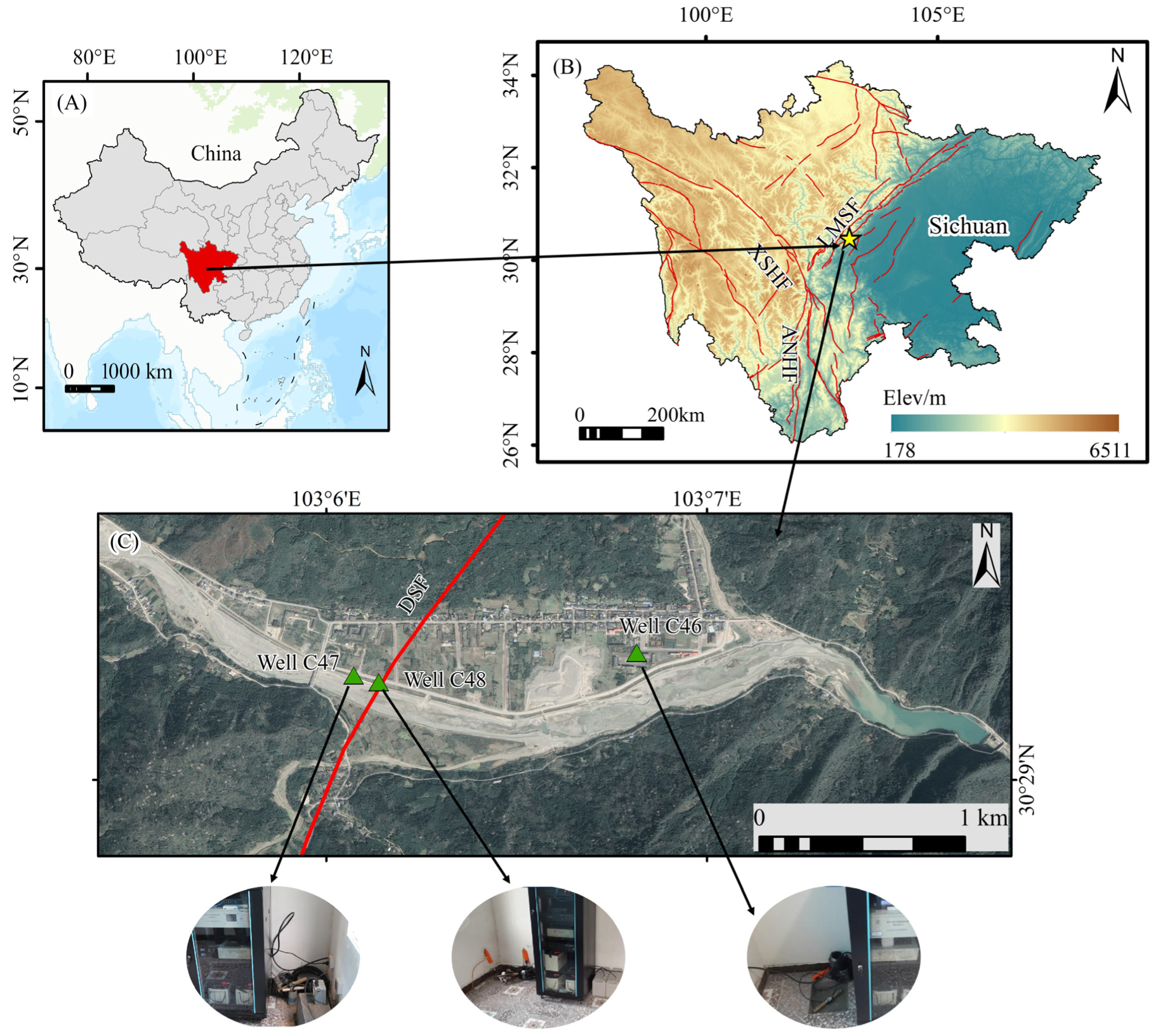
2.1. Study Area Background

The Longmenshan Fault Zone (LMSF) is a prominent tectonic boundary demarcating the eastern margin of the Tibetan Plateau and the northwestern periphery of the Sichuan Basin. As one of China’s most active fault systems, it exhibits complex structural configurations and intense seismotectonic activity. The LMSF has generated multiple significant seismic events in the 21st century [37], including the 2013 Lushan (M_S 7.0) earthquake and the 2022 Lushan (M_S 6.1) earthquake. The two earthquakes both occurred along the southern segment of the LMSF and resulted in substantial human casualties and economic losses [38]. Therefore, this study focuses on the frontal-range fault of the southern LMSF, or the DSF (Figure 1). The DSF extends approximately 140 km along a NE (40°) strike with a NW dip, spanning from northeastern Dayi to southwestern Tianquan through Dachuan, Taiping, and Shuangshi. This thrust fault system is characterized by an imbricate structure accompanied by numerous subsidiary faults [39]. Three adjacent monitoring wells (C47, C48, and C46 (Figure 1C)), drilled in July 2014, were positioned across different structural domains of the DSF. This distribution enables a comparative analysis of seismic hydrogeological response characteristics across the fault zone. The C47 well is situated in the hanging wall, C48 within the fault fracture zone, and C46 in the footwall, with inter-well spacing of approximately 110 m and 1100 m, respectively.

The schematic wellbore configurations and lithological characteristics of the three groundwater monitoring wells are shown in Figure 2. These wells employ standardized open-hole completions with consistent 80 mm diameters for both casing and open-hole sections. Specific configurations are as follows: (1) well C47 (depth of 161.4 m) features an open-hole interval spanning 100.8–161.4 m, penetrating an aquifer system dominated by diabase–diorite complexes interbedded with limestone; (2) well C48 (depth of 125.6 m) contains an open-hole section from 76.0 m to total depth, intersecting a Triassic clastic sequence comprising sandstone–mudstone limestone, with a prominent fault damage zone identified at a depth of 41.8–75.5 m; (3) well C46 (depth of 160.3 m) exhibits stratigraphic continuity with well C48, maintaining equivalent aquifer lithology while extending its open-hole interval from 98.3 m to total depth. Systematic monitoring revealed stable borehole conditions throughout the observational period, with no detectable serious destruction from natural events or anthropogenic disturbances.

2.2. Data Sources

2.2.1. Water Level Data

The water levels of the three groundwater observation wells were measured using the ZKGD3000-N digital instrument (Beijing Zhongkeguangda Automation Technology Co., Ltd., Beijing, China), which has a measurement range of 0–50 m, an accuracy of ±0.2% F.S., a stability of ±0.1% F.S., and a resolution better than 1 mm. We collected continuous water level raw data from 1 January 2020 to 31 December 2023. The raw data underwent quality control through the manual removal of anomalous steps and spikes caused by anthropogenic disturbances or instrument malfunctions, as documented in the observation logs. Figure 3 presents the time series of dynamic water level change data. The water level fluctuations in all three observation wells exhibited seasonal patterns, primarily driven by heavy summer precipitation. This resulted in significant water level rise during the rainy season (May–July), establishing an annual cycle characterized by higher water levels in summer and lower levels in winter. The water level data can be obtained from the database of the Sichuan Geophysical Network Center.

2.2.2. Earthquake Events

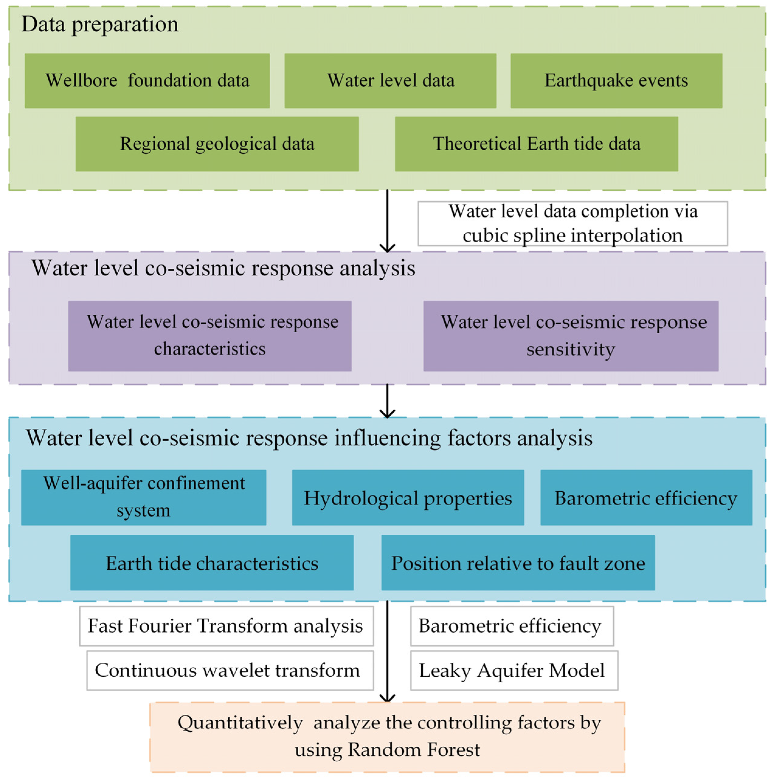
The earthquake parameters were obtained from the China Earthquake Networks Center (https://news.ceic.ac.cn/, accessed on 31 January 2024), and the event selection followed spatial criteria: (1) M_S ≥ 4.0 events within a 200 km radius of the observation wells; (2) M_S ≥ 5.0 events within a 500 km radius; (3) M_S ≥ 6.0 events within a 1000 km radius; and (4) global M_S ≥ 7.0 events. All selected events occurred between 1 January 2020 and 31 December 2023. Based on the above selection criteria, a total of 90 earthquake events were selected in this study, and the results are presented in

Table 1. Statistics of earthquake frequency.

MS	4.0~5.0	5.1~6.0	6.1~7.0	7.1~8.0	≥8.0
Frequency	21	6	18	44	1

.

2.3. Methods

In this study, the characteristics and sensitivity of the water level co-seismic response of the three wells were analyzed, and then RF was used to quantitatively evaluate the importance of the factors controlling the sensitivity of the water level co-seismic response. The involved factors primarily include hydraulic parameters, aquifer confinement, fault architecture, tidal characteristics, and barometric efficiency. The research process is shown in Figure 4.

2.3.1. Well–Aquifer Confinement Based on Tidal Response

The co-seismic response sensitivity of well water levels is closely associated with the confinement capacity of the well–aquifer system [28,30]. Spectral analysis based on the tidal response of well water levels serves as an effective method to determine aquifer confinement [40]. The water level fluctuations are influenced by the Earth’s tides and the five principal tidal constituents (M₂, S₂, N₂, K₁, and O₁), accounting for approximately 95% of the total tidal potential energy. Typically, the aquifer is determined to be confined when the tidal response of the water level is mainly affected by the Earth’s tide; the amplitudes of the five main components are obvious, and the amplitude of the M₂ tidal wave is the most significant. Semi-confined aquifer systems are characterized by intermediate S₂, K₁, and M₂ components, and the O₁ and N₂ components may appear attenuated or absent. In contrast, unconfined aquifer systems typically display negligible or undetectable tidal components [41,42]. The Baytap-08 program [43] is mainly used to extract tidal parameters. This program adopts the condition of minimizing the Akaike Bayesian information criterion (ABIC) method to calculate corresponding tidal parameters by obtaining the optimal fit between observed data. The observed well water level data can be decomposed into the following components:

$$y_i={\displaystyle \sum _{m=1}^M({\alpha }_m{C}_{mi}+{\beta }_m{S}_{mi})+}{\displaystyle \sum _{k=1}^K{\mathrm{b}}_k{x}_{i-k}}+d_i+e_i$$

(1)

where the right side of the equation represents the tidal component, the barometric response component, the trend term, and the random noise term of the water level data. $C_{mi}$ and $S_{mi}$ are the theoretical calculated values of the tidal component of order $m$, ${\alpha }_m$ and ${\beta }_m$ are the corresponding tidal response coefficients, $x_{i-k}$ is the observed pressure, and ${\mathrm{b}}_k$ is its response coefficient.

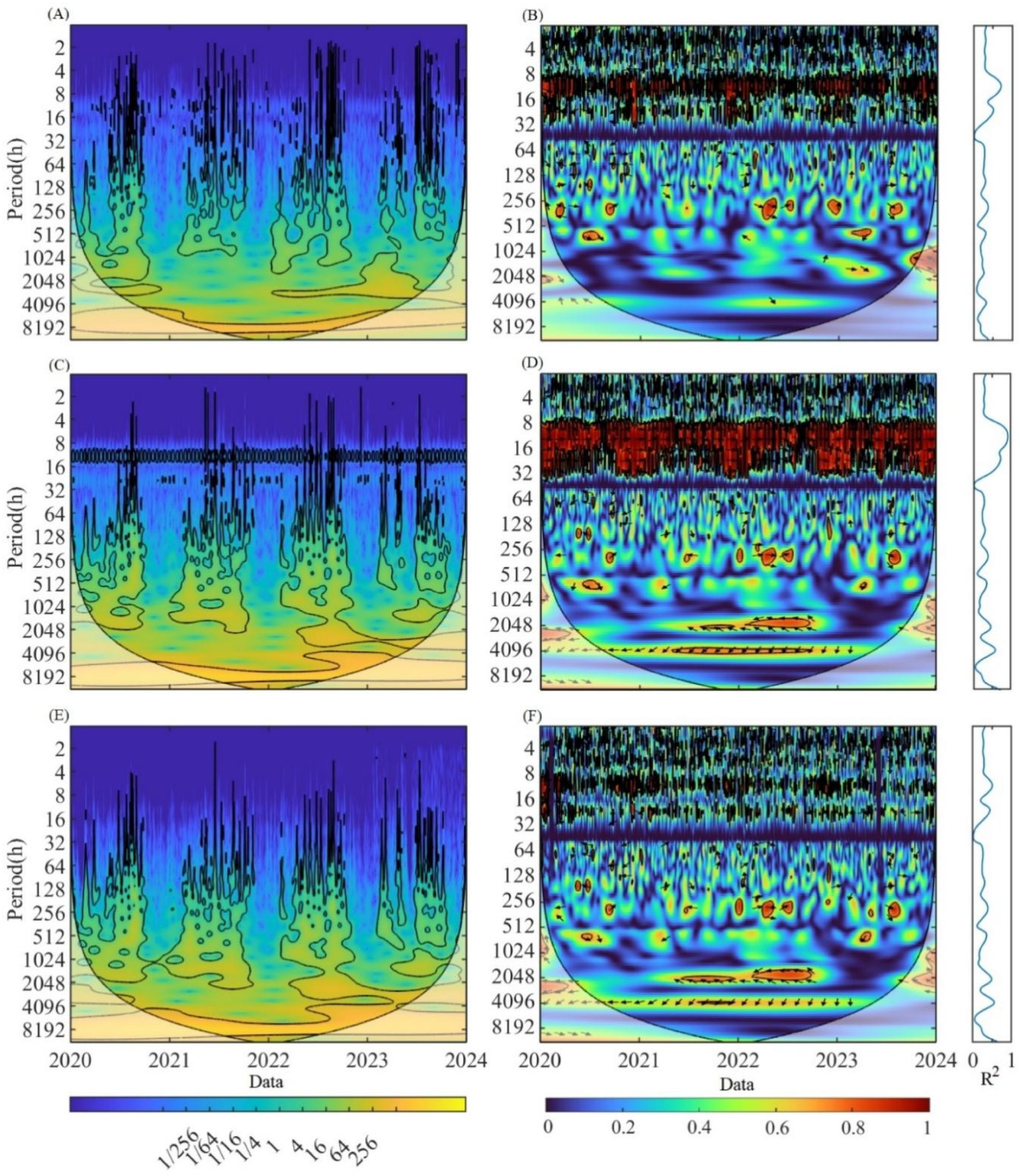
2.3.2. Continuous Wavelet Coherence

Continuous wavelet transform (CWT) analysis serves as a powerful mathematical tool for characterizing periodic dynamic components of well water level time series through time–frequency domain decomposition. This technique enables the quantitative characterization of spectral response characteristics in well water level time series data, particularly for identifying dominant periodicities in hydrogeological signals [28]. The wavelet coherence function further enhances this analytical capability, which is particularly valuable for investigating interactions between periodic groundwater fluctuations and mechanisms driving the Earth’s tides. The wavelet coherence can be defined as:

$$R^2(x,y)={\displaystyle \frac{{\left|S(s^{-1}W(x,y))\right|}^2}{S(s^{-1}W(x))·S(s^{-1}W(y))}}$$

(2)

$$W_n^X=\sqrt{{\displaystyle \frac{\delta t}{s}}}{\displaystyle \sum _{n\prime =1}^N{x}_{n\prime }\phi }\left[(n\prime -n){\displaystyle \frac{\delta t}{s}}\right]$$

(3)

where $R^2$ is the wavelet coherence coefficient, which ranges from 0 to 1, corresponding to the water level and tide time series coherence from small to large; $W(x)$ and $W(y)$ are continuous wavelet transformations of the water level and tide time series, respectively; $W(x,y)$ is the cross-wavelet transform of the water level and tide time series; $S$ is the smoothing operator; $x_{n\prime }$ is the time series of the well water level; $\delta t$ is the length of the time series; $\phi (x)$ is the wavelet function; $s$ is the wavelet scale; and $N$ is the number of convolution times per Fourier space.

2.3.3. Leaky Aquifer Model

In the natural environment, many aquifers may often involve simultaneous coupled vertical and radial flows. To address such complex aquifers and the tidal response of concurrent horizontal flows and vertical leakage conditions, Wang et al. [24] proposed a tidal response model for leaky aquifers that is closer to natural conditions to resolve groundwater responses to the Earth’s tides. The leaky aquifer model assumes that the aquifer is laterally extensive and that flows through the semi-confining aquitard are vertical. Under such constraints, the specific leakage ($\sigma$), which quantifies the aquitard’s vertical transmission capacity, (defined as $\sigma$ = ${\displaystyle \frac{k\prime }{b\prime }}$, where $b\prime$ and $k\prime$ are the thickness and the vertical hydraulic conductivity of the aquitard, respectively) can be evaluated by the following equation:

$$T({\displaystyle \frac{{\partial }^{2}h}{\partial r^2}}+{\displaystyle \frac{1}{r}}{\displaystyle \frac{\partial h}{\partial r}})-{\displaystyle \frac{k\prime }{b\prime }}h=S({\displaystyle \frac{\partial h}{\partial t}}-{\displaystyle \frac{B{k}_u}{\rho g}}{\displaystyle \frac{\partial \epsilon }{\partial t}})$$

(4)

where $b$ and $k$ are the thickness and hydraulic conductivity of the aquifer, respectively. $r$ is the radial distance from the studied well. $h$ is the hydraulic head in the aquifer above a common reference. $T$ and $S$ are the transmissivity and storativity of the aquifer, respectively. $\epsilon$ is the tidal oscillating volumetric strain of the aquifer. $B$ and $k_u$ are the Skempton’s coefficient and the undrained bulk modulus of the aquifer, respectively.

This equation has three independent parameters: $T$ and $S$ for the aquifer and ${\displaystyle \frac{k\prime }{b\prime }}$ for the semi-confining aquitard, which are related to the phase shift ($\eta$) and the amplitude ratio ($A$) of the response to the tidal response for the specific borehole. We define the $\eta$ and $A$ as:

$$A=\left|{\displaystyle \frac{i\omega S}{(i\omega S+k\prime /b\prime )\xi }}\right|$$

(5)

$$\eta =\arg [{\displaystyle \frac{i\omega S}{(i\omega S+k\prime /b\prime )\xi }}]$$

(6)

where

$$\xi =1+{({\displaystyle \frac{r_c}{r_w}})}^2{\displaystyle \frac{i\omega r_w}{2T\beta }}{\displaystyle \frac{K_0(\beta r_w)}{K_1(\beta r_w)}}$$

(7)

$$h_{w,0}={\displaystyle \frac{i\omega S}{(i\omega S+k\prime /b\prime )\xi }}({\displaystyle \frac{B{K}_u{\epsilon }_0}{\rho g}})$$

(8)

where $\omega$ is the angular frequency (regarded as a constant in the case of a specific tidal wave component). $r_c$ is the case pipe radius of the well and $r_w$ is the filter pipe radius of the well. $\arg (z)$ is the argument of the complex number $z$.

By integrating the $\eta$ and $A$ parameters derived from tidal response analyses with continuous water level data, the leaky aquifer tidal model enables the quantitative evaluation of permeability evolution in aquifer systems.

2.3.4. Barometric Efficiency

Barometric efficiency (B_p) is defined as the ratio of the water level fluctuation amplitude to atmospheric pressure variation under undrained aquifer conditions [44]. It can serve as a quantitative index for characterizing an aquifer’s responsivity to atmospheric pressure. When atmospheric pressure variations occur, water exchange occurs between the wellbore and the aquifer to equilibrate the pressure differential [42,45]. The B_p of well water levels provides an effective approach for evaluating the aquifer’s sensitivity to crustal stress changes across fault zones. For aquifers, higher B_p values correlate with reduced stress sensitivity due to an enhanced pressure-buffering capacity [46,47]. Clark [48] used the observed atmospheric pressure change $\mathrm{\Delta }b$ and water level change $\mathrm{\Delta }h$ to determine the barometric efficiency value in constant time increments:

$$BE={\displaystyle \frac{{\displaystyle \sum \mathrm{\Delta }h}}{{\displaystyle \sum \mathrm{\Delta }b}}}={\displaystyle \frac{S_h^i}{S_b^i}}$$

(9)

where

$$S_b^i=S_b^{i-1}+\left|\mathrm{\Delta }{b}_i\right|$$

(10)

$$S_h^i=\left\{\begin{array}{ccc}{S}_h^{i-1}-\left|\mathrm{\Delta }{h}_i\right|& & (\beta i>0)\\ S_h^{i-1}+\left|\mathrm{\Delta }{h}_i\right|& & (\beta i<0)\\ S_h^{i-1}& & (\beta i=0)\end{array}\right.$$

(11)

where $S_h^i$ and $S_b^i$ are the sum of the atmospheric pressure change and water level change, respectively.

$$\mathrm{\Delta }{b}_i=b_i-b_i-1$$

(12)

$$\mathrm{\Delta }{h}_i=h_i-h_i-1$$

(13)

$${\beta }_i=\mathrm{\Delta }b\cdot \mathrm{\Delta }{h}_i$$

(14)

where $b_i$ and $h_i$ are the atmospheric pressure and water level at time $t_i$, and ${\beta }_i$ is the product of atmospheric change value $\mathrm{\Delta }b$ and water level change value $\mathrm{\Delta }h$ at time $t_i$.

2.3.5. Random Forest

Random forest (RF) [36] is an ensemble learning algorithm and is widely applied to classification, regression, and feature importance evaluation tasks. It operates by an ensemble of multiple decision trees that are constructed using random feature subsets. The mean decrease accuracy (MDA) of RF is one of the importance evaluation methods used to assess quantifying feature importance. This method evaluates the contribution of each feature by measuring the average decline in prediction accuracy when the feature’s values in out-of-bag (OOB) samples are randomly permuted to disrupt their original associations. If the accuracy of a feature outside the bag decreases significantly after the permutation, it indicates that the importance of this feature is relatively high. For unimportant features, the effect is the opposite. The MDA score for feature $j$ is calculated as follows:

$$MA{D}_j={\displaystyle \frac{{\displaystyle \sum _{i=1}^N(OOBee{r}_2(i)-OOBee{r}_{er1}(i))}}{N}}$$

(15)

where $N$ denotes the total number of decision trees. $OOBee{r}_2(i)$ and $OOBee{r}_1(i)$ represent the classification accuracy of the $i$-th tree before and after permuting feature j, respectively.

3. Results and Discussion

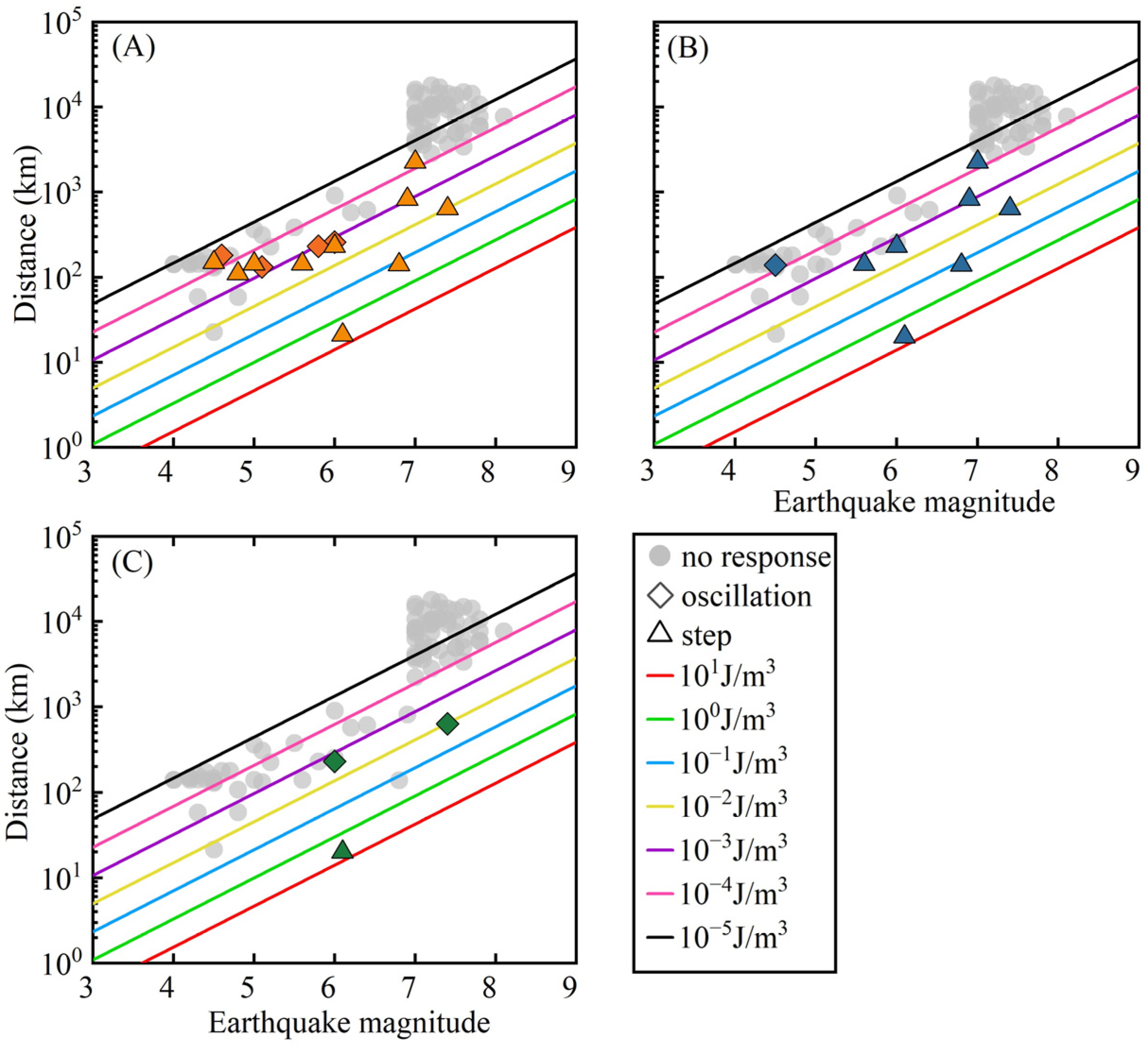
3.1. Response to Earthquakes

We examined the response of the water level to these selected earthquakes. The earthquake events and co-seismic response characteristics of water levels in the three fluid observation wells are statistically summarized in

Table 2. Features of water level co-seismic response changes of the three fluid observation wells.

ID	Date and Time	Earthquake	MS	Water Well Stations
				Well C46			Well C47			Well C48
				EP	Amp	Res	EP	Amp	Res	EP	Amp	Res
1	2020/2/3 0:05	qingbaijiang	5.1	132	1.9	oscillation	-	-	-	-	-	-
2	2020/10/21 12:04	beichuan	4.6	181	1.3	oscillation	-	-	-	-	-	-
3	2021/5/22 2:04	maduo	7.4	639	113.8	step fall	639	118.9	step fall	639	1	Oscillation
4	2021/9/16 4:33	luxian	6	258	1.9	oscillation	-	-	-	-	-	-
5	2022/1/8 1:45	menyuan	6.9	828	8.9	gradual fall	828	1	gradual rise	-	-	-
6	2022/5/20 8:36	hanyuan	4.8	110	20.1	gradual fall	-	-	-	-	-	-
7	2022/6/1 17:00	lushan	6.1	21	308.1	step rise–step fall	20	220.8	step fall–gradual rise	20	13.1	step rise
8	2022/6/10 0:03	maerkang	5.8	233	2.8	oscillation	-	-	-	-	-	-
9	2022/6/10 1:28	maerkan	6	231	7	step fall	231	2.4	step fall	231	2	oscillation
10	2022/7/27 8:43	Philippines	7	2268	4.6	step rise	2269	7.8	step rise	-	-	-
11	2022/9/5 12:52	luding	6.8	141	73.6	step fall	140	21.5	step fall	-	-	-
12	2022/9/7 2:42	shimian	4.5	150	2.9	step rise	-	-	-	-	-	-
13	2022/10/22 13:17	luding	5	143	4.9	step fall	-	-	-	-	-	-
14	2023/1/26 3:49	luding	5.6	143	25.2	step fall	142	2.4	gradual rise	-	-	-
15	2023/5/12 2:34	luding	4.5	-	-	-	139	1.1	oscillation	-	-	-

Note: M_S is the magnitude of the earthquake, EP represents the epicenter distance (km), Amp represents the amplitude of the water level co-seismic change (mm), Res represents response polarity, and “-” means no co-seismic changes.

. The C46 well exhibited the highest sensitivity, recording 14 co-seismic events. These included 11 near-field earthquakes (Sichuan, China) and two strong seismic events (Qinghai, China). Notably, it detected the 27 July 2022 Philippines Earthquake (M_S 7.0) at an epicentral distance of 2268 km, marking the farthest recorded response. The C47 well registered eight co-seismic events, with four events showing polarity consistent with the C46 well. Additionally, the C47 well uniquely captured the 12 May 2023 Luding (M_S 4.5) earthquake. In contrast, the C48 well demonstrated limited co-seismic sensitivity, recording only three events: the 22 May 2021 Maduo (M_S 7.4), 10 June 2022 Maerkang (M_S 6.0), and 1 June 2022 Lushan (M_S 6.1) earthquakes.

We also quantified the co-seismic sensitivity of the three groundwater observation wells to earthquakes across magnitude–distance domains (

Table 3. Statistics on the co-seismic response event ratios of the three fluid observation wells, classified by magnitude.

Magnitude Division	Seismic Events	Water Well Stations
		Well C46			Well C47			Well C48
		Response Times	Ratio (%)	Maximum Distance (km)	Response Times	Ratio (%)	Maximum Distance (km)	Response Times	Ratio (%)	Maximum Distance (km)
4 ≤ MS < 5	19	3	15.79	181	1	5.26	139	0	0	-
5 ≤ MS < 6	8	4	50	233	1	12.50	142	0	0	-
6 ≤ MS < 7	8	5	62.5	828	4	50	828	2	25	231
7 ≤ MS < 8	54	2	3.7	2268	2	3.7	2269	1	1.85	639
MS ≥ 8	1	0	0	-	0	0	-	0	0	-

Note: “-” means not available.

). Significant differences emerged in their sensitivity profiles: The C46 well demonstrated superior sensitivity, responding to 26% of regional M_S < 6.0 events at approximately 200 km and 34% of M_S < 7.0 events at approximately 800 km. The C47 well exhibited moderate sensitivity, detecting 17% of M_S < 7.0 earthquakes at approximately 800 km. The C48 well showed localized sensitivity limited to M_S ≥ 6.0 events at approximately 200 km and M_S ≥ 7.0 events at approximately 600 km. All wells displayed negligible responses to distant seismicity (>2000 km epicentral distance), with only the 27 July 2022 Philippines M_S 7.0 earthquake (epicentral distances: C46 = 2268 km and C47 = 2269 km) triggering measurable anomalies in the C46 and C47 wells.

According to Roeloffs et al. [49], water level changes may be related to the magnitude of each earthquake and its distance from the well. The relationship between the well’s water level and the seismic magnitude, as well as the well–epicentral distance, can be fitted by the following form:

$$\lg \mathrm{\Delta }{h}_i=b_1{M}_S+b_2\lg D+a$$

(16)

where $\mathrm{\Delta }{h}_i$ represents water level changes; $D$ is the well–epicentral distance; $M_S$ is the seismic magnitude; and $b_1$, $b_2$, and $a$ are constants.

Because the C48 well’s limited sample data preclude its use for regression analysis, only the C46 and C47 wells were included in the multiple linear regression analysis. The multiple linear regression results are as the

Table 4. Multiple linear regression analysis.

	Variable	Regression Coefficients
		Unstandardized Coefficients		Unstandardized Coefficients	t	Sig
		B	Std. Error	Beta
$\lg \mathrm{\Delta }{h}_{C46}$	constant	−0.271	0.772		−0.351	0.732
	$M_S$	0.715	0.147	0.924	4.870	0.000 **
	$\lg D$	−1.249	0.295	−0.804	−4.239	0.001 **
$\lg \mathrm{\Delta }{h}_{C47}$	constant	−1.645	1.569		−1.048	0.342
	$M_S$	−1.151	0.435	−0.797	−2.648	0.046 *
	$\lg D$	0.849	0.290	0.881	2.925	0.033 *

Note: $\mathrm{\Delta }{h}_{C46}$ and $\mathrm{\Delta }{h}_{C47}$ are the water level changes of wells C47 and C46, respectively. * p < 0.05, ** p < 0.01

:

The results show that the water level change amplitudes of the two wells have good correlations with the seismic magnitude and the well–epicentral distance. However, the fluid co-seismic response amplitude exhibits differences. In the earthquakes simultaneously recorded by both the C46 and C47 wells, it was observed that C46 generally exhibited larger co-seismic response amplitudes compared to C47. The reason for this difference might be that the differences in hydrogeological structural conditions around the well locations have a significant impact on the co-seismic water level response.

3.2. Co-Seismic Response Sensitivity

Seismic energy density (e), defined as the maximum energy flux per unit volume transferred from seismic waves to geological media during propagation [50], serves as a critical parameter for quantifying co-seismic hydrogeological responses. In theory, the intensity of seismic wave energy acting on geological formations directly correlates with the magnitude of co-seismic responses observed in well water levels [51]. Under stable wellbore structures and consistent hydrogeological conditions, a distinct threshold of seismic energy density exists, beyond which earthquakes can induce detectable responses in well water levels. Lower thresholds typically indicate a higher sensitivity of fluid observation wells to seismic activities [19,52]. Wang and Manga [50] established a global threshold of 10⁻³ J/m³ for sustained groundwater level responses triggered by seismic events. Analysis of the scatter plot depicting the epicenter distance versus magnitude (Figure 5) reveals that the seismic energy densities capable of eliciting co-seismic water level responses in the C46 well predominantly range between 10⁻³ J/m³ and 10⁻⁵ J/m³. Notably, when the seismic energy density exceeds 10⁻³ J/m³, the co-seismic response in the C46 well primarily manifests as a step change. Conversely, at lower energy densities (<10⁻³ J/m³), the response may vary, exhibiting oscillations, step changes, or in some cases, no detectable response. The C47 well demonstrates a similar range of triggering seismic energy densities to the C46 well, with most responses characterized by step changes, and an exception was observed during the 12 May 2023, Luding earthquake (M_S 4.5), where the response manifested as an oscillation. In contrast, the C48 well exhibits fewer recorded instances of co-seismic responses, particularly at seismic energy densities exceeding 10⁻³ J/m³, suggesting a comparatively lower sensitivity to seismic events than the C46 and C47 wells.

Consequently, sensitivity rankings followed the sequence C46 > C47 > C48, establishing C46 as the most seismically responsive monitoring station in the groundwater monitoring network.

3.3. Water Level Co-Seismic Response Mechanism

We took the 1 June 2022, Lushan (M_S 6.1) earthquake and the 22 May 2021, Maduo (M_S 7.4) earthquake as the representative earthquake events for the near-field region and mid-to-far-field region earthquake response mechanism analysis, respectively. The water level co-seismic response characteristics are shown in Figure 6.

The co-seismic response mechanism of groundwater levels involves a complex interplay of multiple factors. From the spatial distribution perspective, the dominant mechanisms exhibit notable regional variations [53].

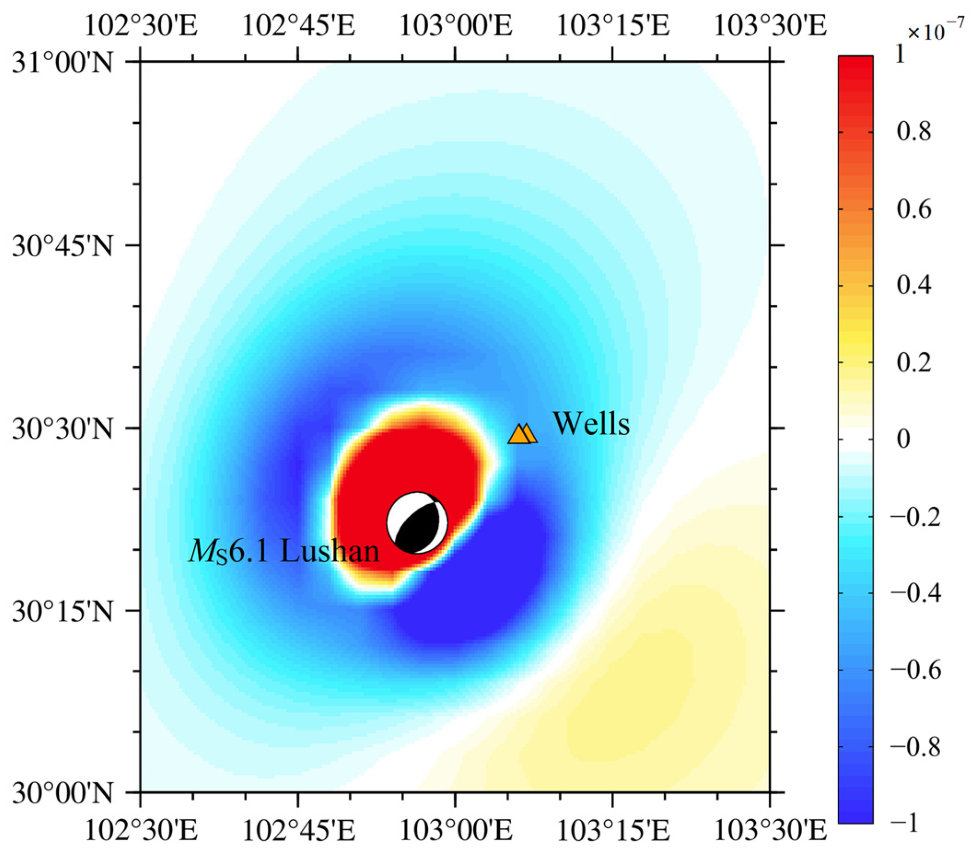
3.3.1. The Near-Field Region

In the 1 June 2022 Lushan (M_S 6.1) earthquake, the three groundwater observation wells exhibited different co-seismic response characteristics. The C46 well demonstrated step rise–step fall characteristics. In contrast, the C47 well displayed step fall–gradual rise response characteristics. The C48 well showed a step-rise response characteristic. In the near-field region earthquake, both static and dynamic stress fields contributed to the observed effects, with the static stress field exerting a more significant influence. Based on Okada’s dislocation theory [54], we calculated the co-seismic strain fields of this earthquake, and the results are illustrated in Figure 7. It can be found that the wells are situated within the co-seismic strain contraction zones. Alterations in the co-seismic static stress field directly impact the stress distribution within aquifers, prompting adjustments in pore pressure and resulting in step-like changes in water levels [55,56]. These changes generally align with the direction of the co-seismic strain field, as evidenced by observations in borehole wells C46 and C48. It is noteworthy that the C47 well, located within a contraction zone, displayed a co-seismic decrease in water levels [57]. This phenomenon may involve more intricate multi-stage processes, such as fracture formation or unblocking [58], which necessitate further investigation.

3.3.2. The Mid-To-Far-Field Region

In the 22 May 2021 Maduo (M_S 7.4) earthquake, minor oscillatory characteristics were observed in well C48. In contrast, the C46 and C47 wells recorded obvious step-like declines. In the mid-to-far-field region, the mechanisms differ markedly from those in the near-field. Owing to the greater distance from the epicenter, the influence of the static stress field is considerably diminished, and the dynamic stress field generated during the propagation of seismic waves emerges as the predominant driving factor [53,59]. Under the influence of seismic waves, the permeability of the aquifer may undergo changes, potentially in the direction of either the upward or downward hydraulic gradient, leading to random fluctuations in water levels, which may rise, fall, or just oscillate [5,28].

In practical observations, the response characteristics are contingent upon the relative strength of each mechanism and the specific hydrogeological conditions of the local environment [19,28,34].

3.4. Factors Influencing Response Sensitivity

The spatial proximity of the three groundwater observation wells (with inter-well distances of approximately 110 m and 1100 m, respectively) enables effective isolation of the influence of the seismic wave constituents when assessing co-seismic response sensitivity. The hydrological co-seismic response sensitivity induced by earthquakes may be influenced by factors such as the hydrogeological conditions and the geological structural characteristics. These will be discussed in the following sections on their relative control over the co-seismic response.

3.4.1. Influence of the Well–Aquifer Confinement System

Fast-Fourier transform analysis was performed on the water levels of the three groundwater observation wells (Figure 8). The analysis revealed distinct tidal components in well C47, with clearly identifiable M₂ and S₂ waves, where the M₂ component demonstrated the largest amplitude of 12.29 mm. Furthermore, O₁ and K₁ tidal components were also distinctly observed in well C47, confirming its operation within a favorable confined aquifer system. In contrast, well C46 exhibited only M₂ and S₂ components with relatively smaller tidal amplitudes, suggesting a semi-confined aquifer system. Notably, well C48 showed no discernible tidal components in its groundwater level frequency spectrum, indicating a poorly confined aquifer system. This classification as an unconfined well–aquifer system likely explains the relatively weaker co-seismic response sensitivity observed in well C48 compared to the other two wells.

According to previous studies, wells with well-confined aquifer systems typically possess a relatively enclosed spatial structure that facilitates efficient fluid pressure transmission [28]. This characteristic enables them to effectively reflect various crustal stress-strain changes and produce significant responses to seismic wave-induced micro-dynamic information [26,60,61]. Generally, wells with greater confinement capacities demonstrate stronger amplification sensitivities to crustal stress–strain fluctuations and thus tend to show more sensitivity to seismic stress [62], which is inconsistent with our observations. Well C47, despite possessing a favorable well–aquifer system, exhibited less pronounced co-seismic response sensitivity compared to well C46, which has a relatively inferior well–aquifer system. This finding leads us to believe that while the confinement degree of the aquifer system may influence the sensitivity of the well water level to the co-seismic response, it may be a contributory factor rather than a decisive dominant factor.

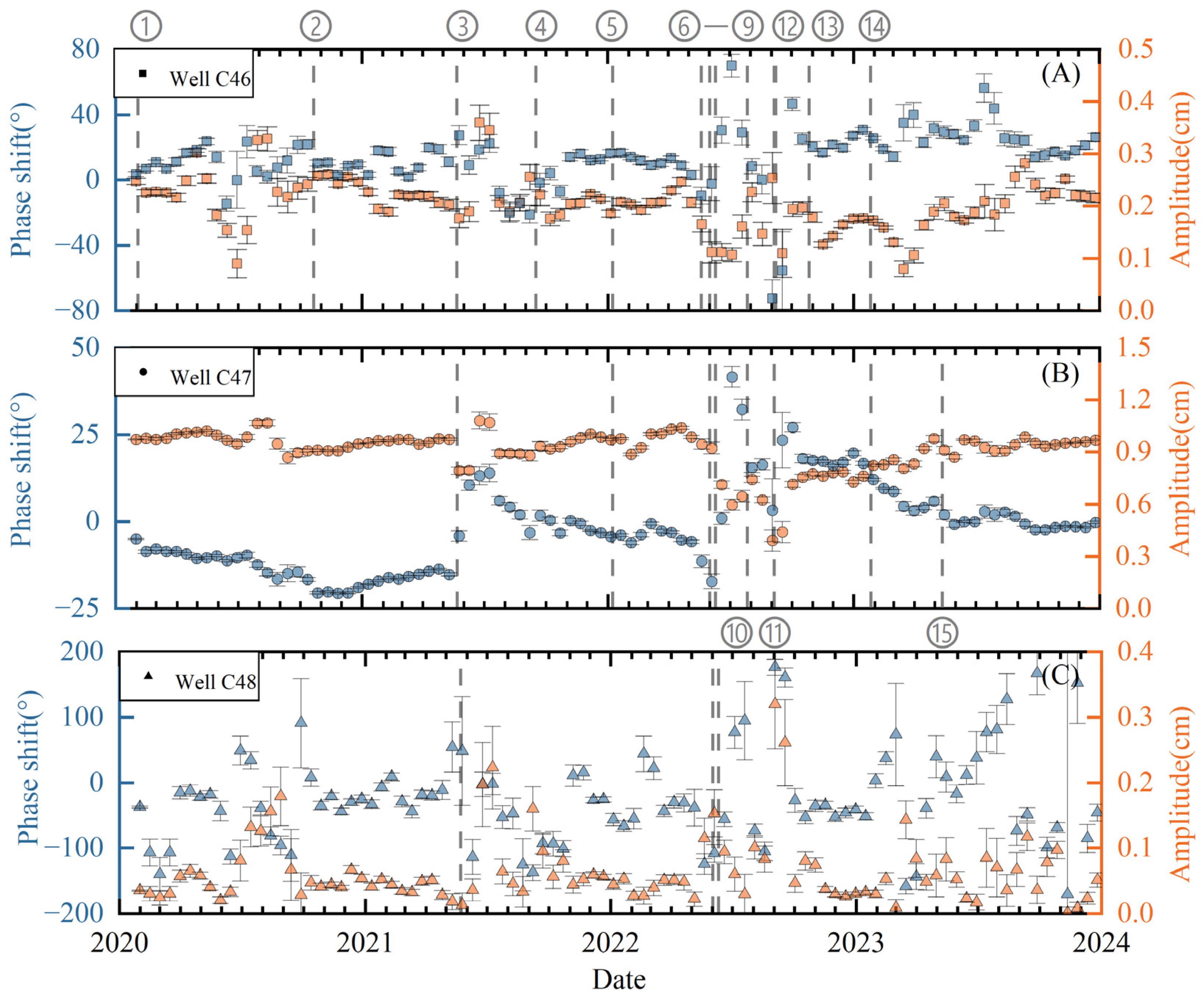
3.4.2. Influence of the Characteristics of the Earth’s Tides

Before performing the continuous wavelet transform analysis, we filled the water level data gaps via cubic spline interpolation and then calculated the continuous wavelet power spectrum to identify the periodic components of the water level (Figure 9). All three groundwater observation wells exhibited dominant semi-annual (~4096 h) and annual (~8192 h) periodicities, consistent with seasonal hydrological factors. Well C46 displayed persistent semi-diurnal (~12 h) and diurnal (~24 h) Earth tide signals, but these signals were attenuated by stronger seasonal energy components. Well C47 revealed coherent semi-diurnal tidal energy clusters (“bead structures”) but lacked discernible diurnal signatures. In contrast, well C48 showed no statistically significant tidal signals. Simultaneously, we calculated the hourly values of the theoretical Earth tides during the same period and conducted a wavelet coherence analysis with the water level. The wavelet coherence analysis between the water level and Earth tides showed that the water levels of wells C46 and C47 are strong and basically stable in the semi-diurnal wave periodic component. Well C46 exhibited moderate correlations (R = 0.5~0.7), whereas well C47 maintained stronger and stable coherence across 8~32 h periods (R = 0.8~0.9), confirming tidal dominance in hydraulic fluctuations. In contrast, well C48 displayed negligible coherence across all frequency bands, suggesting a poor wavelet correlation throughout the whole period. This observation is consistent with those reported in previous studies where aquifer systems that showed poor responsiveness to the periodic loading of the Earth’s tides are also expected to show a low sensitivity to seismic stress [28,63]. Therefore, well C48 exhibits a lower co-seismic response sensitivity than the other two wells.

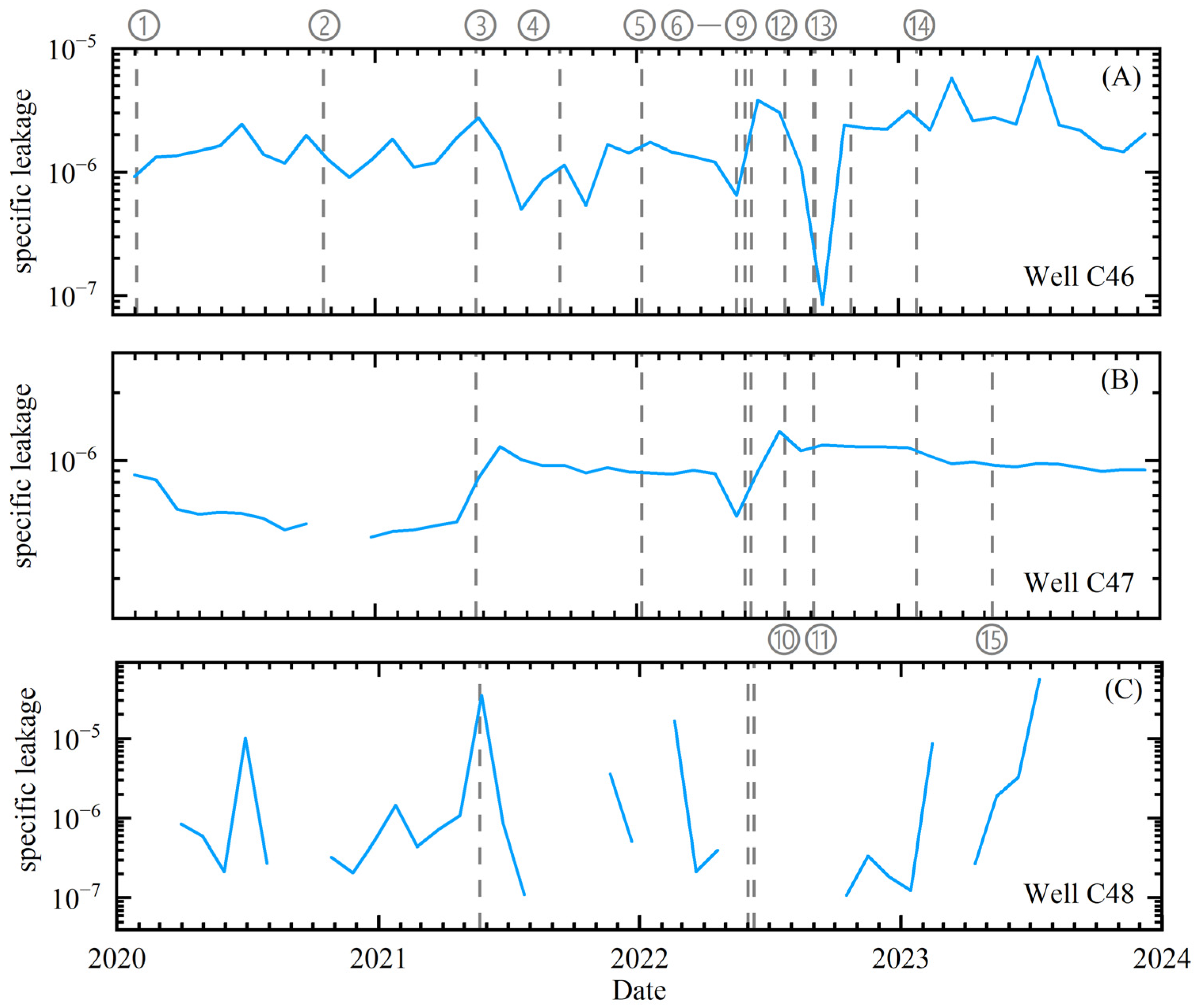
3.4.3. Influence of Hydrological Properties

Tidal analysis of fluid observation wells provides a quantitative evaluation of co-seismic response variability across well–aquifer systems [28,34]. Therefore, we used the responses of the water level to the Earth’s tides to quantify the changes in the parameters of the aquifer system. The M₂ tidal constituent, driven by lunar gravitational forcing, exhibits a stable amplitude with minimal modulation from temperature or barometric effects, making it ideal for investigating aquifer tidal responses [22]. Utilizing the Baytap-08 tidal analysis program [43], we computed temporal variations in M₂ tidal phase lags and amplitudes using a 30-day sliding window with a 15-day step length (Figure 10). Pronounced tidal parameter variations reflect permeability changes in aquifer systems, where increasing phase shifts indicate enhanced aquifer permeability [34]. Preceding the 2021 Maduo M_S 7.4 earthquake, well C47 exhibited a characteristic phase lag surge, indicative of horizontal flow dynamics in confined aquifers. In contrast, well C46 predominantly displayed positive phase shifts, consistent with vertical flow-dominated systems interspersed with radial flow components. Well C48 displays relatively complex dynamic fluctuations in phase shift and amplitude, reflecting heightened hydraulic instability. The differences in the distinct dynamic fluctuations of amplitudes and phase shifts between the three fluid observation wells are ascribed to the changes in the aquifers’ hydrological properties.

To quantitatively calculate the variation of the aquifers’ hydrological properties, we used the leakage aquifer model to calculate the $\sigma$, and the results are shown in Figure 11. The $\sigma$ with large deviations are excluded to maintain accuracy. For well C46, the $\sigma$ exhibited relative stability, with values varying from 7 × 10⁻⁷ to 10⁻⁵ prior to the 1 June 2022 Lushan (M_S 6.1) earthquake. Notably, significant fluctuations were observed from May to September 2022, which may be attributed to the enhanced seismic activity during this period. The $\sigma$ of well C47 was stable within the range of 2 × 10⁻⁷ to 2 × 10⁻⁶ and fluctuated slightly under the perturbations of the earthquakes. However, the $\sigma$ of well C48 demonstrated heightened deviations and uncertainty, varying from1 4 × 10⁻⁸ to 9 × 10⁻⁵. This condition may be attributed to the well’s unique geological setting within the fault damage zone, where the aquifer’s hydraulic characteristics demonstrated heightened vulnerability to disturbances [21,30,64].

The hydraulic gradients around the fault zone are quite different. When wells are very close together, the changes in the hydraulic parameters of the well–aquifer system caused by earthquakes may be quite different. Previous studies have reported that the discrepancies in hydraulic parameter magnitudes within aquifers play a crucial role in modulating the sensitivity of the groundwater level response to earthquakes [31,58,63]. The $\sigma$ of well C46 is larger than that of well C47, suggesting that well C46 could be more sensitive to the periodic loading by seismic waves; therefore, the distinct co-seismic response sensitivity of the wells can be attributed to varying hydraulic parameters.

3.4.4. Influence of Barometric Efficiency

The B_p calculation involved the following steps: first, we removed the trend components of the data, then applied the Clark method [48] for B_p determination. The atmospheric pressure imbalance between well water and the adjacent aquifer causes the well water level to fluctuate, and the response of the well water level to atmospheric pressure fluctuations is instantaneous. Therefore, we calculated B_p values for the period of one month before each earthquake and took the average as the final barometric efficiency. The results revealed that B_p C47 > B_p C46 > B_p C48, with the detailed values presented in

Table 5. Barometric efficiency of the monitoring wells.

Data	Water Well Stations
	Bp C46	Bp C47	Bp C48
Average value	0.87	2.33	−0.73

.

The fault zone fracture forms a rapid pressure conduction channel, which responds to stress changes through rapid fluid discharge. Theoretical studies on barometric efficiency [47] have established an inverse relationship between a well’s B_p and its aquifer’s sensitivity to stress and strain. Generally, aquifers with high B_p values indicate strong aquifer buffering stability, which effectively reduces stress-induced water level changes. Conversely, aquifers with lower Bp values indicate a significant reduction in pressure-buffering capacity, and the aquifer is highly sensitive to stress perturbations. Based on this theory and our calculations, we conclude that the aquifer associated with well C46 demonstrates higher sensitivity than well C47’s aquifer. This finding is consistent with the previous study of Song et al. [46] that a well with a higher B_p was less sensitive to the stress changes in its aquifer.

3.4.5. Influence of Position Relative to the Fault Zone

The fault zone forms a structurally anisotropic network with distinct spatial orientation characteristics, developing multiscale fracture systems that constitute primary conduits for groundwater migration. Aquifer-connected fractures within fault zones exert significant control over seismic-induced water level fluctuations [21]. The DSF exhibited a general NE (40°) strike, and we drew the azimuth map of earthquakes along the strike of the fault (Figure 12). Co-seismic monitoring data reveal systematic spatial variations in response sensitivity among observation wells. Well C46 demonstrates robust co-seismic response capabilities for recording nine earthquakes on the fault’s footwall side and five events on the hanging wall side. In contrast, well C47 exhibits pronounced sensitivity to seismic activity on the hanging wall side of the fault zone, documenting seven earthquakes and registering only one significant event on the opposite side. Well C48, however, shows limited recording capacity, detecting only three seismic events, all of which occurred on the hanging wall side of the fault zone.

This spatial distribution of seismic responses provides valuable insights into the fault zone’s hydrogeological characteristics. The sensitivity hierarchy (C46 > C47 > C48) correlates with structural positions relative to the fault architecture. This response sensitivity appears to be governed by the fault’s hydraulic architecture and its interaction with seismic wave propagation characteristics. The diminished response capacity of well C48 is located within the fault fracture zone [24,65]. Comparatively, wells positioned in relatively intact hanging wall (well C47) and footwall (well C46) blocks maintain enhanced hydraulic connectivity. This observation aligns with previous studies showing that wells within a fault damage zone are more vulnerable than those away from the fault damage zone and thus have poor sensitivity to seismic stress [28,30,46,66].

3.5. Importance Analysis of Influencing Factors

RF was employed to quantitatively assess the importance of influencing factors. The input characteristic variables were five influencing factors: (1) hydraulic parameters, (2) aquifer confinement, (3) fault architecture, (4) tidal characteristics, and (5) barometric efficiency. For hydraulic parameters and B_p values, the 30-day average values before each earthquake are calculated as the input values according to the seismic data in Table 2. Tidal characteristics represent the response of the water level to tides. This factor was quantified through the wavelet coherence coefficient between the water level and the Earth’s tides within the band between 8 hr and 32 hr (the semi-diurnal and diurnal components) one month before each earthquake. The confinement degree of the well–aquifer system is assigned 0, 0.5, and 1 according to confinement and unconfinement. Similarly, the fault architecture is assigned 1, 0, and −1 according to the hanging wall, the fault fracture zone, and the footwall. All the input feature parameters are normalized prior to modeling. We visualized the importance of influence factors by using RF to classify the seismic data into co-seismic responses and non-co-seismic responses according to Table 2. Meanwhile, we randomly split the data into a training set and a test set in a ratio of 7:3. The test set does not participate in the model-building process. The accuracy and ROC AUC were used to verify classification performance. The model results show that the accuracy rate of the training set reaches 92%, while that of the test set reaches 81.2%. The ROC AUC value of the model reaches 0.74, which indicates that the classification prediction results of the model are relatively good. Therefore, the feature importance results have reference significance.

We visualized the feature factors’ importance, and the results are shown in

Table 6. The importance analysis results of influencing factors by RF.

Hydraulic Parameters	Aquifer Confinement	Fault Architecture	Tidal Characteristics	Barometric Efficiency
0.4	0.24	0.17	0.13	0.06

. The feature importance analysis reveals that the factors that affect the water level’s co-seismic response sensitivity, in descending order of importance, include hydraulic parameters, aquifer confinement, the fault architecture, tidal characteristics, and barometric efficiency. Hydraulic parameters and aquifer confinement account for 64% of the importance of all factors. They are the main controlling factors affecting the difference in the water level’s co-seismic response sensitivity collectively. Tide characteristics and the fault architecture have relatively similar importance, and both exhibit lower importance than hydraulic parameters and aquifer confinement. On the contrary, the response of atmospheric pressure is relatively weak, indicating that it is not a key factor affecting the water level’s co-seismic response sensitivity compared to other influencing factors.

The quantitative evaluation shows that vertical permeability is an important hydrological property that controls the transportation processes of groundwater in shallow crust. Highly permeable aquifers are more responsive to the stress disturbances of seismic waves, which is the main influencing factor in the seismic–hydrogeological response process. An increase in vertical permeability facilitates hydraulic communication among aquifers. The well–aquifer confinement system affects the process of seismic stress, changing pore pressure, and pore elasticity, and possibly also hindering the horizontal fluid migration induced by seismic stress, resulting in an insignificant or non-responsive water level response to seismic waves. These findings are of great significance to understanding the mechanisms and characteristics underlying earthquake-related hydrological responses in fault zones.

Furthermore, the depth of well C48 is lower than that of wells C46 and C47, and these structural differences may affect the water level’s co-seismic response. However, previous studies have indicated that the influence of wells’ structural factors on the water level’s co-response is highly uncertain [28,66,67]. In comparison to the dominant factors previously discussed, the well’s structure has a limited influence, as the influence of the well’s structure on the water level’s response to seismic activity may be masked by many factors [31]. For example, the effects of the well structure may be potentially masked by the aquifer’s hydrogeological properties or the seismic wave.

4. Conclusions

Three adjacent groundwater observation wells, located in distinct structural segments of the DSF, were selected to analyze their respective co-seismic response sensitivities, and to discuss the key controlling factors. The research conclusions are as follows: wells C46 and C47 display heightened sensitivities to seismic events, whereas well C48 exhibits comparatively diminished sensitivities to seismic events. Well C47 exhibits confined aquifer properties and tidal characteristics, which are completely inconsistent with its water level’s co-seismic response sensitivity. The specific leakage of well C46 is larger than that of well C47 and is prone to fluctuations under the influence of earthquakes. Based on the quantitative evaluation results, we suggest that the important factors that mainly affect water level responses to seismic events include hydraulic parameters and aquifer confinement. Barometric efficiency exerts a minimal influence on water level co-seismic response sensitivity.

These findings provide support for optimizing the placement of groundwater monitoring wells in seismotectonic environments. Thus, when designing new seismic groundwater observation wells, the hydrogeological environment and aquifer conditions should be comprehensively considered, which could facilitate the capture of weak stress and strain changes to aid potential earthquake precursor information. Furthermore, both sides of the DSF blocks maintain enhanced hydraulic connectivity between the aquifer and connected fractures. Therefore, the second sampling rate of groundwater level monitoring systems can be carried out in the two walls of the DSF blocks to obtain more detailed water level change information. The leaky aquifer model was utilized to calculate the specific leakage to assess the vertical permeability changes caused by earthquakes, which offers an effective approach for estimating aquifer parameter changes.

Given the limited sample size available for analysis regarding these events’ co-seismic response records within wells, the inference results may deviate from actual occurrences. Therefore, these findings require further validation through more examples of co-seismic response records in future research endeavors. Heavy rainfall can cause large changes in the water level and trigger earthquakes via the mechanism of pore pressure diffusion. In the future, we may analyze the correlation between anomalous extreme rainstorms and seismicity. Meanwhile, we may also consider combining geochemical analyses to increase our understanding of the relationship between water and earthquakes.

References

1. Manga, M.; Wang, C.-Y. Earthquake hydrology. Treatise Geophys. 2007, 4, 293–320. [Google Scholar]
2. Wang, C.-Y.; Manga, M. Earthquakes influenced by water. In Water and Earthquakes; Springer: Berlin/Heidelberg, Germany, 2021; pp. 61–82. [Google Scholar]
3. He, A.; Singh, R.P. Groundwater level response to the Wenchuan earthquake of May 2008. Geomat. Nat. Hazards Risk 2019, 10, 336–352. [Google Scholar] [CrossRef]
4. Lai, G.; Jiang, C.; Han, L.; Sheng, S.; Ma, Y. Co-seismic water level changes in response to multiple large earthquakes at the LGH well in Sichuan, China. Tectonophysics 2016, 679, 211–217. [Google Scholar] [CrossRef]
5. Sun, X.; Wang, G.; Yang, X. Coseismic response of water level in Changping well, China, to the Mw 9.0 Tohoku earthquake. J. Hydrol. 2015, 531, 1028–1039. [Google Scholar] [CrossRef]
6. Skelton, A.; Andrén, M.; Kristmannsdóttir, H.; Stockmann, G.; Mörth, C.-M.; Sveinbjörnsdóttir, Á.; Jónsson, S.; Sturkell, E.; Guðrúnardóttir, H.R.; Hjartarson, H.; et al. Changes in groundwater chemistry before two consecutive earthquakes in Iceland. Nat. Geosci. 2014, 7, 752–756. [Google Scholar] [CrossRef]
7. Chi-Yuen, W.; Michael, M. New streams and springs after the 2014 Mw6.0 South Napa earthquake. Nat. Commun. 2015, 6, 7597. [Google Scholar]
8. Yan, X.; Shi, Z.; Zhou, P.; Zhang, H.; Wang, G. Modeling Earthquake-Induced Spring Discharge and Temperature Changes in a Fault Zone Hydrothermal System. J. Geophys. Res. Solid Earth 2020, 125, e2020JB019344. [Google Scholar] [CrossRef]
9. Chen, L.; Zhu, G.; Lin, X.; Li, R.; Lu, S.; Jiao, Y.; Qiu, D.; Meng, G.; Wang, Q. The Complexity of Moisture Sources Affects the Altitude Effect of Stable Isotopes of Precipitation in Inland Mountainous Regions. Water Resour. Res. 2024, 60, e2023WR036084. [Google Scholar] [CrossRef]
10. Li, R.; Zhu, G.; Lu, S.; Meng, G.; Chen, L.; Wang, Y.; Huang, E.; Jiao, Y.; Wang, Q. Effects of cascade hydropower stations on hydrologic cycle in Xiying river basin, a runoff in Qilian mountain. J. Hydrol. 2025, 646, 132342. [Google Scholar] [CrossRef]
11. Fan, X.; Scaringi, G.; Korup, O.; West, A.J.; Westen, C.J.; Tanyas, H.; Hovius, N.; Hales, T.C.; Jibson, R.W.; Allstadt, K.E.; et al. Earthquake-Induced Chains of Geologic Hazards: Patterns, Mechanisms, and Impacts. Rev. Geophys. 2019, 57, 421–503. [Google Scholar] [CrossRef]
12. Shrestha, B.R.; Khanal, N.R.; Smadja, J.; Fort, M. Geo-hydrological hazards induced by Gorkha Earthquake 2015: A Case of Pharak area, Everest Region, Nepal. Geogr. J. Nepal 2020, 13, 91–106. [Google Scholar] [CrossRef]
13. Fan, X.; Westen, C.J.v.; Korup, O.; Gorum, T.; Xu, Q.; Dai, F.; Huang, R.; Wang, G. Transient water and sediment storage of the decaying landslide dams induced by the 2008 Wenchuan earthquake, China. Geomorphology 2012, 171–172, 58–68. [Google Scholar] [CrossRef]
14. Cui, P.; Dang, C.; Zhuang, J.-Q.; You, Y.; Chen, X.-Q.; Scott, K.M. Landslide-dammed lake at Tangjiashan, Sichuan province, China (triggered by the Wenchuan Earthquake, May 12, 2008): Risk assessment, mitigation strategy, and lessons learned. Environ. Earth Sci. 2012, 65, 1055–1065. [Google Scholar] [CrossRef]
15. Hong-jian, Z.; Xi, W.; Yi, Y. Risk Assessment of Disaster Chain: Experience from Wenchuan Earthquake-induced Landslides in China. J. Mt. Sci. 2015, 12, 1169–1180. [Google Scholar]
16. Jacquemond, L.; Godano, M.; Cappa, F.; Larroque, C. Interplay Between Fluid Intrusion and Aseismic Stress Perturbations in the Onset of Earthquake Swarms Following the 2020 Alex Extreme Rainstorm. Earth Space Sci. 2024, 11, e2024EA003528. [Google Scholar] [CrossRef]
17. Mansouri Daneshvar, M.R.; Freund, F.T. Survey of a relationship between precipitation and major earthquakes along the Peru-Chilean trench (2000–2015). Eur. Phys. J. Spec. Top. 2021, 230, 335–351. [Google Scholar] [CrossRef]
18. Nie, W.; Tian, C.; Song, D.; Liu, X.; Wang, E. Disaster process and multisource information monitoring and warning method for rainfall-triggered landslide: A case study in the southeastern coastal area of China. Nat. Hazards 2024, 121, 2535–2564. [Google Scholar] [CrossRef]
19. Shi, Z.; Wang, G.; Manga, M.; Wang, C.-Y. Mechanism of co-seismic water level change following four great earthquakes–insights from co-seismic responses throughout the Chinese mainland. Earth Planet. Sci. Lett. 2015, 430, 66–74. [Google Scholar] [CrossRef]
20. Lai, G.; Ge, H.; Xue, L.; Brodsky, E.E.; Huang, F.; Wang, W. Tidal response variation and recovery following the Wenchuan earthquake from water level data of multiple wells in the nearfield. Tectonophysics 2014, 619–620, 115–122. [Google Scholar] [CrossRef]
21. Yan, R.; Wang, G.; Ma, Y.; Shi, Z.; Song, J. Local groundwater and tidal changes induced by large earthquakes in the Taiyuan Basin, North China from well monitoring. J. Hydrol. 2020, 582, 124479. [Google Scholar] [CrossRef]
22. Shi, Z.; Wang, G. Hydrological response to multiple large distant earthquakes in the Mile well, China. J. Geophys. Res. Earth Surf. 2014, 119, 2448–2459. [Google Scholar] [CrossRef]
23. Yi, L.C.; Yeeping, C.; Yu, C.P.; Chia, C.Y.; Lin, T.T. Impacts of hydrogeological characteristics on groundwater-level changes induced by earthquakes. Hydrogeol. J. 2018, 26, 451–465. [Google Scholar]
24. Wang, C.Y.; Doan, M.L.; Xue, L.; Barbour, A.J. Tidal response of groundwater in a leaky aquifer—Application to Oklahoma. Water Resour. Res. 2018, 54, 8019–8033. [Google Scholar] [CrossRef]
25. Montgomery, D.R.; Manga, M. Streamflow and water well responses to earthquakes. Science 2003, 300, 2047–2049. [Google Scholar] [CrossRef]
26. Sun, X.; Xiang, Y.; Shi, Z. Changes in permeability caused by two consecutive earthquakes—Insights from the responses of a well-aquifer system to seismic waves. Geophys. Res. Lett. 2019, 46, 10367–10374. [Google Scholar] [CrossRef]
27. Manga, M.; Beresnev, I.; Brodsky, E.E.; Elkhoury, J.E.; Elsworth, D.; Ingebritsen, S.E.; Mays, D.C.; Wang, C.Y. Changes in permeability caused by transient stresses: Field observations, experiments, and mechanisms. Rev. Geophys. 2012, 50, 1–24. [Google Scholar] [CrossRef]
28. Zhang, H.; Shi, Z.; Wang, G.; Yan, X.; Liu, C.; Sun, X.; Ma, Y.; Wen, D. Different sensitivities of earthquake-induced water level and hydrogeological property variations in two aquifer systems. Water Resour. Res. 2021, 57, e2020WR028217. [Google Scholar] [CrossRef]
29. Bense, V.; Gleeson, T.; Loveless, S.; Bour, O.; Scibek, J. Fault zone hydrogeology. Earth-Sci. Rev. 2013, 127, 171–192. [Google Scholar] [CrossRef]
30. Yan, R.; Wang, G.; Shi, Z. Sensitivity of hydraulic properties to dynamic strain within a fault damage zone. J. Hydrol. 2016, 543, 721–728. [Google Scholar] [CrossRef]
31. Sun, X.; Xiang, Y.; Shi, Z.; Hu, X.; Zhang, H. Sensitivity of the response of well-aquifer systems to different periodic loadings: A comparison of two wells in Huize, China. J. Hydrol. 2019, 572, 121–130. [Google Scholar] [CrossRef]
32. Ma, Y.; Wang, G.; Yan, R.; Wang, B.; Yu, H.; Yu, C.; Yue, C.; Wang, Y. Relationship between earthquake-induced hydrologic changes and faults. Water 2021, 13, 2795. [Google Scholar] [CrossRef]
33. Fronzi, D.; Mirabella, F.; Cardellini, C.; Caliro, S.; Palpacelli, S.; Cambi, C.; Valigi, D.; Tazioli, A. The role of faults in groundwater circulation before and after seismic events: Insights from tracers, water isotopes and geochemistry. Water 2021, 13, 1499. [Google Scholar] [CrossRef]
34. Xiang, Y.; Sun, X.; Gao, X. Different coseismic groundwater level changes in two adjacent wells in a fault-intersected aquifer system. J. Hydrol. 2019, 578, 124123. [Google Scholar] [CrossRef]
35. Nalmpantis, C.; Vrakas, D. Machine learning approaches for non-intrusive load monitoring: From qualitative to quantitative comparation. Artif. Intell. Rev. 2019, 52, 217–243. [Google Scholar] [CrossRef]
36. Breiman, L. Random forests. Mach. Learn. 2001, 45, 5–32. [Google Scholar] [CrossRef]
37. Zheng, Y.; Yang, Y.; Ritzwoller, M.H.; Zheng, X.; Xiong, X.; Li, Z. Crustal structure of the northeastern Tibetan plateau, the Ordos block and the Sichuan basin from ambient noise tomography. Earthq. Sci. 2010, 23, 465–476. [Google Scholar] [CrossRef]
38. Zhang, L.; Fu, L.; Liu, A.; Chen, S. Simulating the strong ground motion of the 2022 MS6. 8 Luding, Sichuan, China Earthquake. Earthq. Sci. 2023, 36, 283–296. [Google Scholar] [CrossRef]
39. Chen, L.; Ran, Y.; Wang, H.; Li, Y.; Ma, X. The Lushan Ms 7.0 earthquake and activity of the southern segment of the Longmenshan fault zone. Chin. Sci. Bull. 2013, 58, 3475–3482. [Google Scholar] [CrossRef]
40. Rahi, K.A.; Halihan, T. Identifying aquifer type in fractured rock aquifers using harmonic analysis. Groundwater 2013, 51, 76–82. [Google Scholar] [CrossRef]
41. Qu, S.; Shi, Z.; Wang, G.; Xu, Q.; Zhu, Z.; Han, J. Using water-level fluctuations in response to Earth-tide and barometric-pressure changes to measure the in-situ hydrogeological properties of an overburden aquifer in a coalfield. Hydrogeol. J. 2020, 28, 1465–1479. [Google Scholar]
42. Qi, Z.; Shi, Z.; Rasmussen, T.C. Time-and frequency-domain determination of aquifer hydraulic properties using water-level responses to natural perturbations: A case study of the Rongchang Well, Chongqing, southwestern China. J. Hydrol. 2023, 617, 128820. [Google Scholar] [CrossRef]
43. Tamura, Y.; Sato, T.; Ooe, M.; Ishiguro, M. A procedure for tidal analysis with a Bayesian information criterion. Geophys. J. Int. 1991, 104, 507–516. [Google Scholar] [CrossRef]
44. Liu, W.; Shi, Z.; Lyu, S.; Qi, Z.; Yang, P. Comparison of the Methods of Barometric Efficiency Estimation by Water Level:An Application to Gaoda Well in Yunnan. J. Seismol. Res. 2024, 47, 191–199. [Google Scholar]
45. Zhang, H.; Shi, Z.; Wang, G.; Sun, X.; Yan, R.; Liu, C. Large earthquake reshapes the groundwater flow system: Insight from the water-level response to earth tides and atmospheric pressure in a deep well. Water Resour. Res. 2019, 55, 4207–4219. [Google Scholar] [CrossRef]
46. Song, Y.; Gu, H.; Li, H.; Chi, B. Comparison Analysis of Co-Seismic Response Characteristics of Groundwater Level at Two Sides of Fault: A Case Study of Dahuichang Observation Wells in the Middle of Babaoshan Fault in Beijing. J. Jilin Univ. (Earth Sci. Ed.) 2016, 46, 1815–1822. [Google Scholar] [CrossRef]
47. Zhang, Z.; Zheng, J.; Zhang, G.; Jing, J. Response of water level of confined well to dynamic process of barometric pressure. Chin. J. Geophys. 1989, 32, 539–549. [Google Scholar]
48. Clark, W.E. Computing the barometric efficiency of a well. J. Hydraul. Div. 1967, 93, 93–98. [Google Scholar] [CrossRef]
49. Roeloffs, E.A. Hydrologic precursors to earthquakes: A review. Pure Appl. Geophys. 1988, 126, 177–209. [Google Scholar] [CrossRef]
50. Wang, C.Y.; Manga, M. Hydrologic responses to earthquakes and a general metric. Geofluids 2010, 10, 206–216. [Google Scholar] [CrossRef]
51. Kopylova, G.; Boldina, S. Seismo-Hydrogeodynamic Effects in Groundwater Pressure Changes: A Case Study of the YuZ-5 Well on the Kamchatka Peninsula. Water 2023, 15, 2174. [Google Scholar] [CrossRef]
52. Kopylova, G.; Boldina, S. Effects of seismic waves in water level changes in a well: Empirical data and models. Izv. Phys. Solid Earth 2020, 56, 530–549. [Google Scholar] [CrossRef]
53. Freed, A.M. Earthquake triggering by static, dynamic, and postseismic stress transfer. Annu. Rev. Earth Planet. Sci. 2005, 33, 335–367. [Google Scholar] [CrossRef]
54. Okada, Y. Surface Deformation due to Shear and Tensile Faults in a Half Space. Bull. Seismol. Soc. Am. 1992, 82, 1018–1040. [Google Scholar] [CrossRef]
55. Chia, Y. Changes of Groundwater Level due to the 1999 Chi-Chi Earthquake in the Choshui River Alluvial Fan in Taiwan. Bull. Seismol. Soc. Am 2001, 91, 1062–1068. [Google Scholar] [CrossRef]
56. Jónsson, S.; Segall, P.; Pedersen, R.; Björnsson, G. Post-earthquake ground movements correlated to pore-pressure transients. Nature 2003, 424, 179–183. [Google Scholar] [CrossRef] [PubMed]
57. Shi, Z.; Wang, G.C.; Manga, M.; Wang, C.Y. Continental-scale water-level response to a large earthquake. Crustal Permeability 2012, 15, 324–333. [Google Scholar]
58. King, C.Y.; Azuma, S.; Igarashi, G.; Ohno, M.; Saito, H.; Wakita, H. Earthquake-related water-level changes at 16 closely clustered wells in Tono, central Japan. J. Geophys. Res. Atmos. 1999, 1041, 13073–13082. [Google Scholar] [CrossRef]
59. Bonini, M. Investigating earthquake triggering of fluid seepage systems by dynamic and static stresses. Earth-Sci. Rev. 2020, 210, 103343. [Google Scholar] [CrossRef]
60. Zhao, D.; Zeng, Y.; Sun, X.; Mei, A. Rock Damage and aquifer property estimation from water level fluctuations in wells induced by seismic waves: A case study in X10 Well, Xinjiang, China. Shock. Vib. 2021, 2021, 2137978. [Google Scholar] [CrossRef]
61. He, A.; Singh, R.P.; Sun, Z.; Ye, Q.; Zhao, G. Comparison of regression methods to compute atmospheric pressure and earth tidal coefficients in water level associated with Wenchuan Earthquake of 12 May 2008. Pure Appl. Geophys. 2016, 173, 2277–2294. [Google Scholar] [CrossRef]
62. He, A.; Deng, W.; Singh, R.P.; Lyu, F. Characteristics of hydroseismograms in Jingle well, China. J. Hydrol. 2020, 582, 124529. [Google Scholar] [CrossRef]
63. Zhang, W.; Li, M.; Yang, Y.; Rui, X.; Lu, M.; Lan, S. Implications of groundwater level changes before near field earthquakes and its influencing factors–several earthquakes in the vicinity of the Longmenshan-Anninghe fault as an example. Front. Earth Sci. 2025, 13, 1541346. [Google Scholar] [CrossRef]
64. Xue, L.; Brodsky, E.E.; Erskine, J.; Fulton, P.M.; Carter, R. A permeability and compliance contrast measured hydrogeologically on the San Andreas Fault. Geochem. Geophys. Geosystems 2016, 17, 858–871. [Google Scholar] [CrossRef]
65. Husseini, M.I.; Jovanovich, D.B.; Randall, M.; Freund, L. The fracture energy of earthquakes. Geophys. J. Int. 1975, 43, 367–385. [Google Scholar] [CrossRef]
66. Zhang, J.; Zhao, D.; Xu, Y.; Zhang, X. Comparative Analysis of Water Level Coseismic Response Characteristics in Sichuan Fluid Network. Earthquake 2024, 44, 55–72. [Google Scholar]
67. Weaver, K.C.; Arnold, R.; Holden, C.; Townend, J.; Cox, S.C. A probabilistic model of aquifer susceptibility to earthquake-induced groundwater-level changes. Bull. Seismol. Soc. Am. 2020, 110, 1046–1063. [Google Scholar] [CrossRef]
Figure 1. Location (A) and topographical features (B) of the study area, and (C) locations of the three adjacent fluid observation well sites of C47, C48, and C46. Red lines indicate active faults. LMSF represents the Longmenshan Fault; XSHF represents the Xianshuihe Fault; ANHF represents the Anninghe Fault; and DSF represents the Dachuan-Shuangshi Fault.
Water 17 01568 g001
Figure 2. The simplified completion and lithology profiles of the C47, C48, and C46 wells and boreholes. “↑” points to the depth and lithology of wells.
Water 17 01568 g002
Figure 3. Time series of water level changes of the C46 (A), C47 (B), and C48 (C) wells, recorded from 1 January 2020 to 31 December 2023.
Water 17 01568 g003
Figure 4. Research process roadmap.
Water 17 01568 g004
Figure 5. Seismic energy densities of the C46 (A), C47 (B), and C48 (C) wells.
Water 17 01568 g005
Figure 6. Water level changes in the C46, C47, and C48 wells due to the 2021 MS 7.4 Maduo earthquake and 2022 MS 6.1 Lushan earthquake. The red vertical lines correspond to the earthquake events.
Water 17 01568 g006
Figure 7. Co-seismic static Coulomb stresses of the 2022 MS 6.1 Lushan earthquake. The blue color represents the contraction zone, and the red color indicates the dilation zone. The “beach ball” shows the focal mechanism for the earthquake.
Water 17 01568 g007
Figure 8. Fast-Fourier transforms of the water levels of wells C46 (A), C47 (B), and C48 (C).
Water 17 01568 g008
Figure 9. Continuous wavelet power spectrum of water levels in (A) wells C46, (C) C47, and (E) C48. Wavelet coherence between water levels and the Earth’s tides in (B) wells C46, (D) C47, and (F) C48.
Water 17 01568 g009
Figure 10. Time series of the phase shift and amplitude of the M2 tide component of wells C46 (A), C47 (B), and C48 (C). The error bars show the root mean squared errors. The vertical lines correspond to the origin time of the earthquakes, with the same IDs listed in Table 2.
Water 17 01568 g010
Figure 11. Time series of the σ for wells C46 (A), C47 (B), and C48 (C). The vertical lines correspond to the origin time of the earthquakes, with the same ID listed in Table 2.
Water 17 01568 g011
Figure 12. Azimuth distribution of the co-seismic response events recorded in wells C46 (A), C47 (B), and C48 (C) along the strike of the DSF. The red dashed line denotes the azimuth of the general strike of the DSF.
Water 17 01568 g012