Wetlands as Climate-Sensitive Hotspots: Evaluating Greenhouse Gas Emissions in Southern Chhattisgarh

Abstract

In recent decades, wetlands have played a significant role in the global carbon cycle, making it essential to quantify their greenhouse gas (GHG) emissions at regional, national, and international levels. This study examines three dammed water bodies (Dalpatsagar, Gangamunda, and Dudhawa lake–wetland complexes) in Chhattisgarh, India, to estimate their GHG emission potentials. Methane (CH₄) showed the highest emission rate, peaking at 167.24 mg m⁻² h⁻¹ at 29.4 °C in Dalpatsagar during the standard meteorological week of 21–27 May. As temperatures rose from 17 °C to 18 °C, CH₄ emissions ranged from 125–130 mg m⁻² h⁻¹. Despite slightly higher temperatures, Dudhawa showed lower emissions, likely due to its larger surface area and shallower depth. Carbon dioxide (CO₂) emissions from Gangamunda increased sharply from 124.25 to 144.84 mg m⁻² h⁻¹ as temperatures rose from 12 °C to 25 °C, while Dudhawa recorded a peak CO₂ emission of 113.72 mg m⁻² h⁻¹ in April. Nitrous oxide (N₂O) emissions peaked at 29.11 mg m⁻² h⁻¹ during the 8th meteorological week, with an average of approximately 10.0 mg m⁻² h⁻¹. These findings indicate that climate-induced changes in water quality may increase health risks. This study offers critical insights to inform policies and conservation strategies aimed at mitigating emissions and enhancing the carbon sequestration potential of wetlands.

1. Introduction

Water bodies, including wetlands, ponds, reservoirs, tanks, dams, check dams, and rivers, play vital roles as sources or sinks of atmospheric greenhouse gases (GHGs), including carbon dioxide (CO₂), methene (CH₄), and nitrox oxide (N₂O) [1,2]. Wetland soil also acts as a sink, extending the wet period of any water body that captures a significant amount of carbon in the profiles. In mapping, the carrying capacity of wetlands at the terrestrial level opens a new window for real-time carbon assessment. Temporary and natural water bodies are another issue in trapping carbon in terrestrial water bodies, due to high fluctuations in the release of atmospheric GHG. Among the GHGs, wetlands can release small amounts of CO₂, and human activities in catchment enhance methane emissions, as the global warming potential (GWP) of CH₄ is 25 times greater than that of CO₂, and even warmer soil accelerates the release of CH₄. Wetlands are recognized as carbon storage in the form of biomass [3]; however, they are prominent sources of GHGs (especially CO₂, CH₄) but negligible sources of nitrous oxide (N₂O), which depends on nitrogen loading from the catchments. The IPCC [4] report indicates that the global mean temperature will reach 1.5 °C between 2030 and 2050, and it is assumed that 90% of global warming is due to potent GHG through natural or anthropogenic activities. Notably, the GWP of CH₄ and N₂O are 28 and 310 times greater than that of CO₂, respectively, based on a 100-year IPCC horizon [5]. Wetlands occupy only 6% of the global land surface and act as major sinks for GHGs [6].

India has a diverse range of aquatic resources that comprise an extensive network of 3.15 million ha of reservoirs, 2.36 million ha of ponds and tanks, and 1.2 million ha of floodplain wetlands and lakes [7]. The role of CO₂ and CH₄ in global climate change is widely known in the international scientific domain. Subsequently, the global carbon cycle and indulgent carbon source emissions or sinks have become an interesting research topic; nutrient inputs, such as nitrogen and phosphorus, play critical roles in GHG emissions [2]. Eutrophic water bodies have characteristic features and may exhibit a net influx of atmospheric carbon [2]. Wetlands are generally regarded as significant carbon sinks and account for one-third of universal soil carbon sequestration [8].

Surface waters are universally considered substantial emitters of CO₂, CH₄, and N₂O in the atmosphere [9]. Large water bodies emit 9–27% (70–175 Tg CH₄ yr⁻¹) [10]. In general, benthic sediments emit (diffusion and ebullition) a significant amount of CH₄, and the high availability of organic carbon (OC) and anoxic conditions favor methanogenesis [11]. Typically, nearly 50% of CH₄ emissions from large water bodies occur via diffusion rather than ebullition [9]. Reservoirs, particularly young reservoirs (aged <10 years), have the potential to produce high CO₂ and CH₄ emissions. Created reservoirs are important water bodies and are the largest anthropogenic source of CH₄ (23%) emissions under surface flow, whereas the organic matter (OM) of reservoirs is exhibited as a source of CH₄ and CO₂. Kumar and Bijalwan [12] stated that methane emissions can be controlled by water depth, the chemistry of flooded soil, organic carbon, phosphorus concentrations, etc. Moreover, aquatic denitrification and nitrification change the nitrogen pool and project higher N₂O [13]. Recently, the emission rates of inland water enhanced the CO₂ emission over 2 Pg C yr⁻¹, of which the water body was estimated to be 0.32 to 0.50 Pg C yr⁻¹ [14]. Both ebullition and diffusion (flux) ranged from 0.01 to 52.1 mmol m⁻² d⁻¹, whereas the staged inland water released 0.583 Pg C yr⁻¹; in fact, it accounts for 15.1% of CO₂ emissions and 40.6% of diffusive CH₄ emissions [15].

It is a common assessment that the benthic zone emits (via diffusion and ebullition) a significant amount of CH₄, where the high availability of OC and the anoxic conditions favor methanogenesis. Methane diffusion from benthic deposits in large water bodies is extremely constant in space and time. Diffusive CH₄ fluxes across water columns vary both diagonally and within structures [16]. To further understand the variability in the emission of greenhouse gases, the experiment was framed to study the quantity of their contributions by releasing CO₂, CH₄, and N₂O during the times of the year with the lowest release and the peak release and their responsible factors. Thus, we quantified the magnitude and variability of the emissions over daily timescales. The overall aim was to determine the best method for measuring and quantifying with minimum sampling effort.

2. Materials and Methods

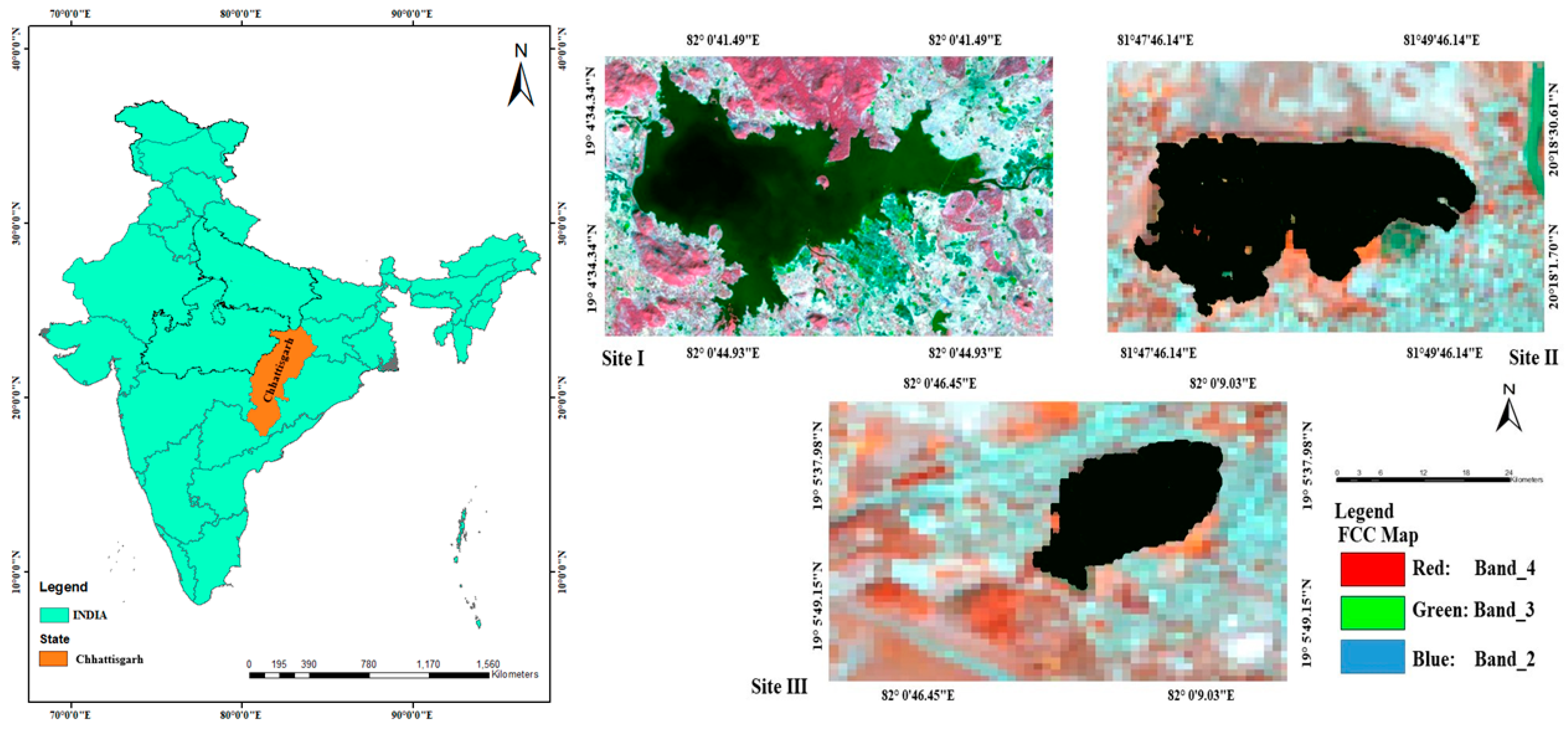
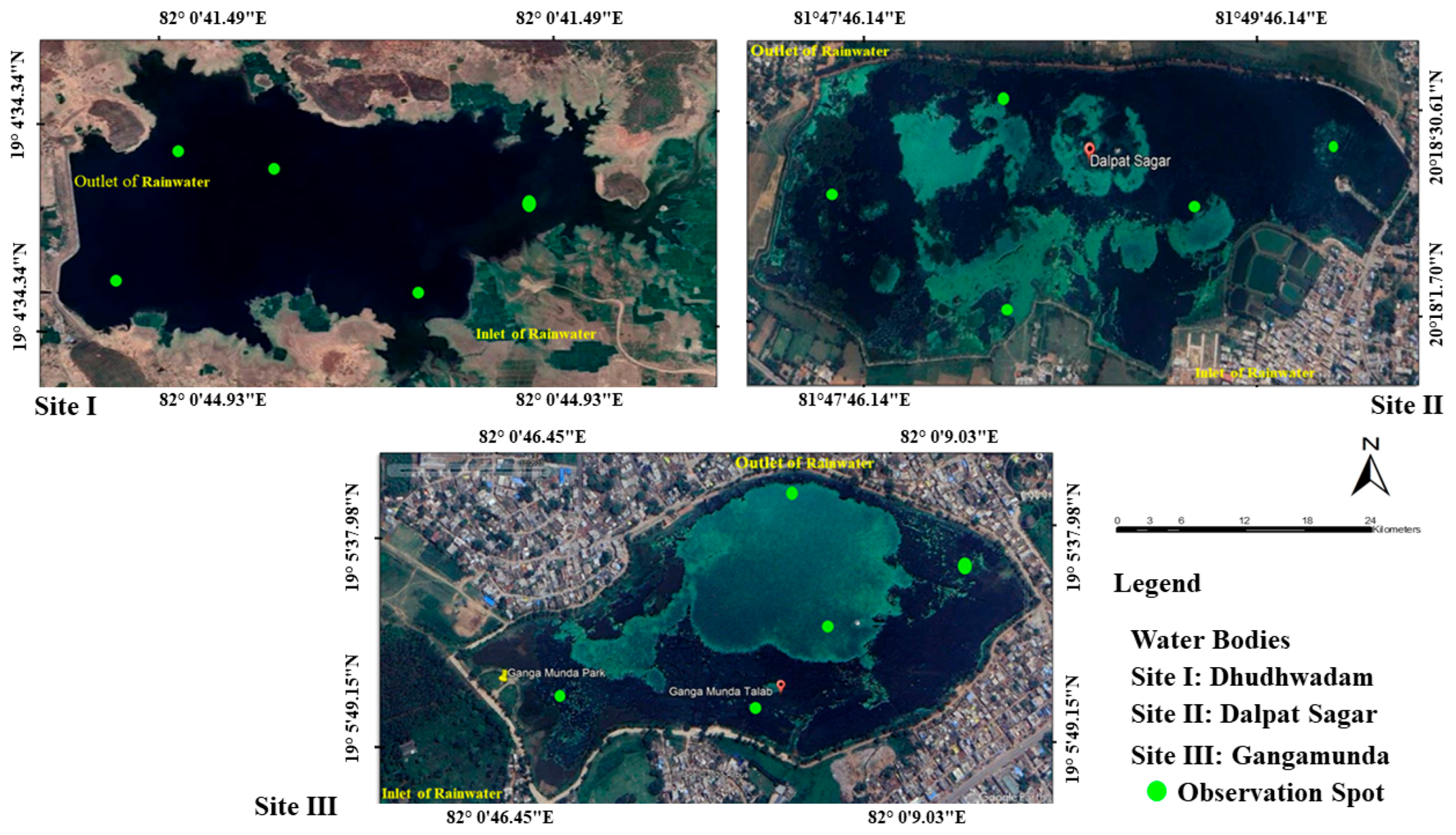
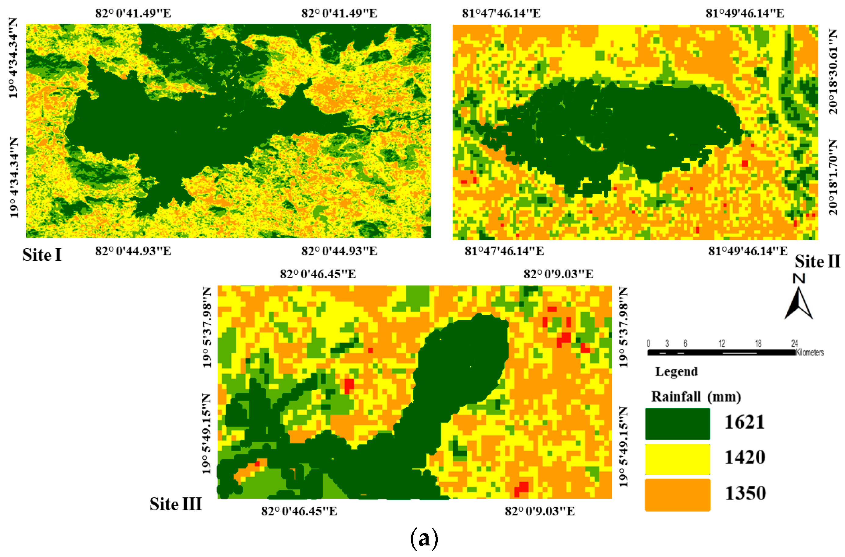
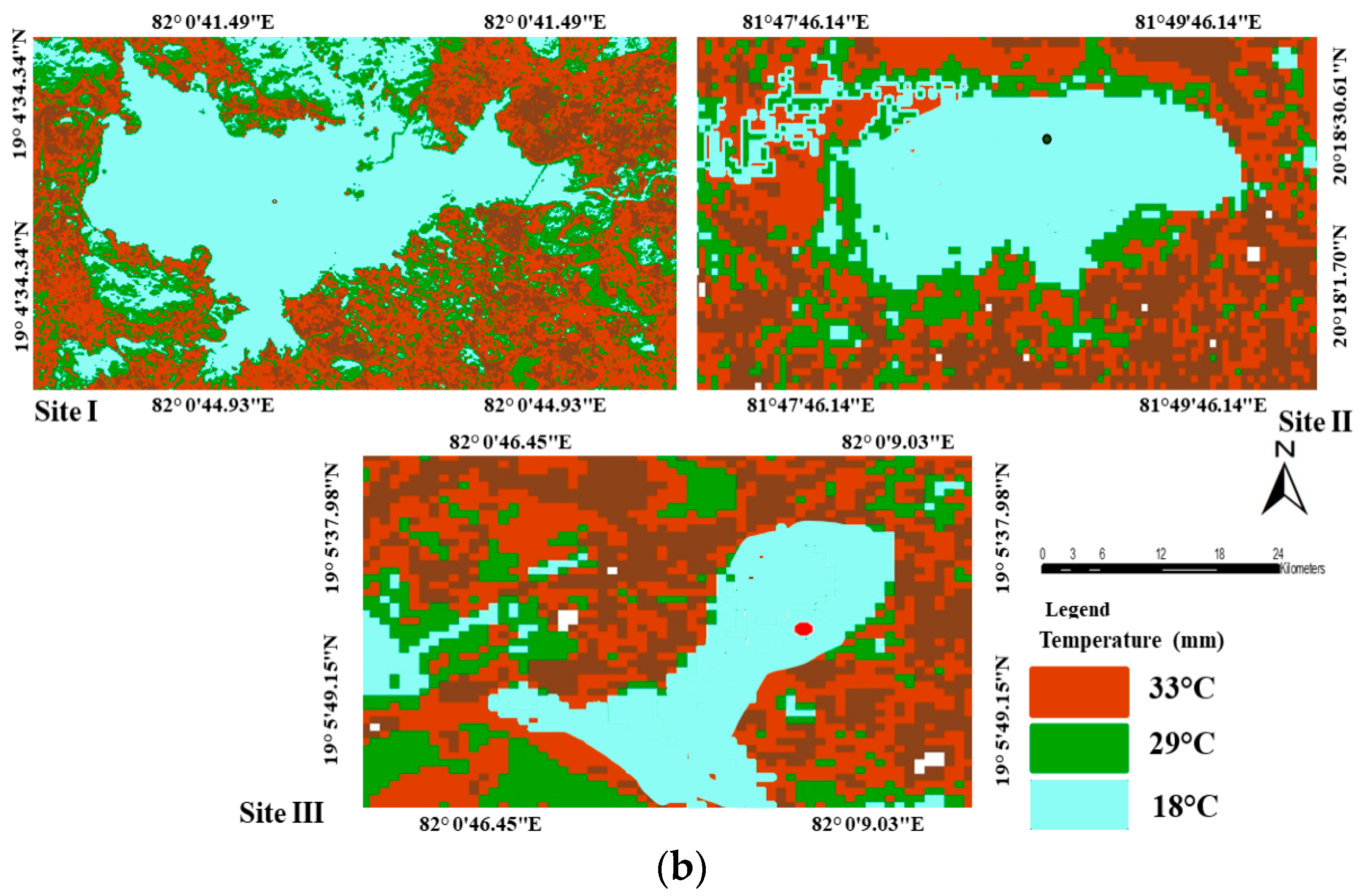
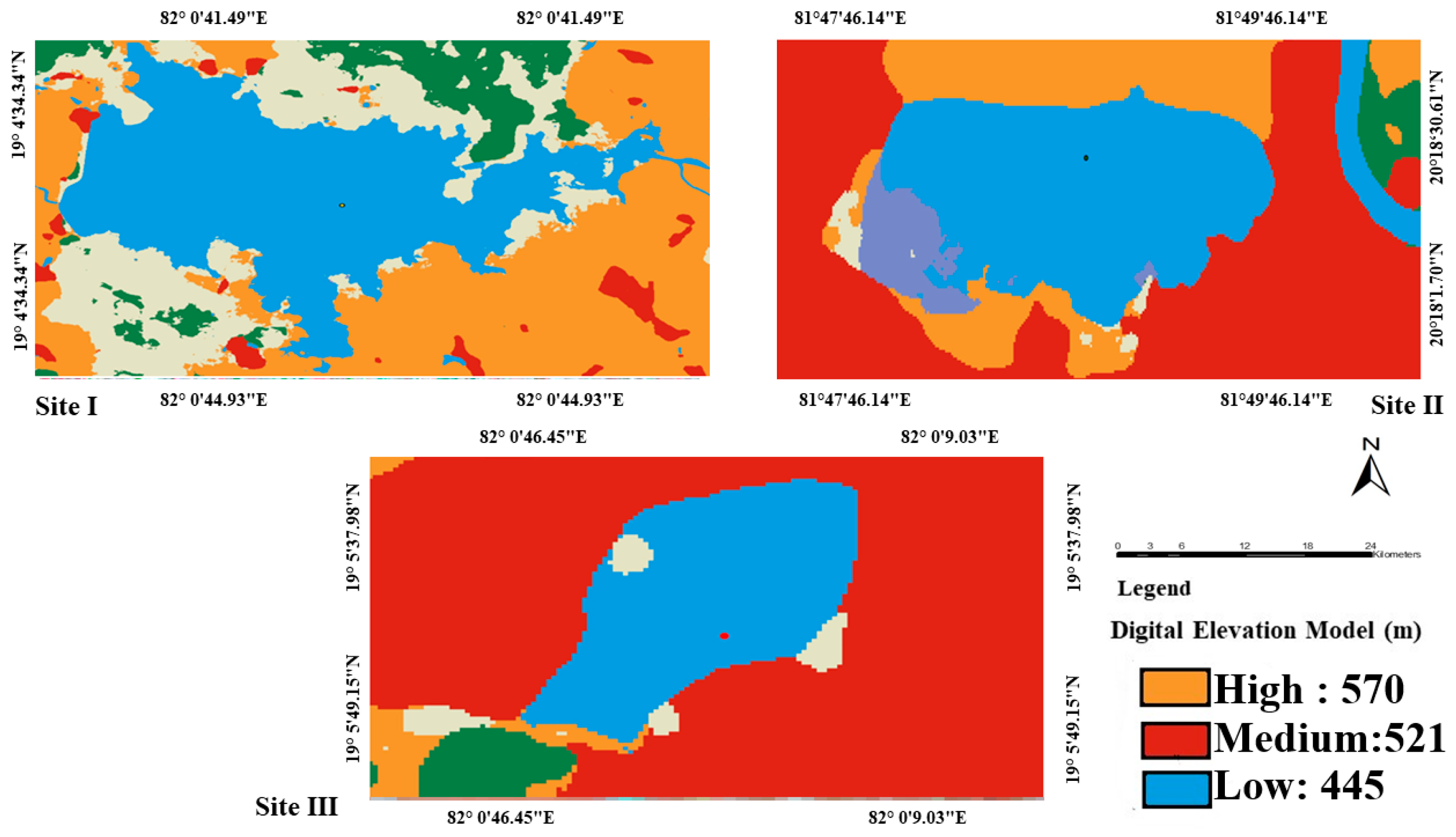
2.1. Study Area

In this study, three water bodies, namely, the Dalpatsagar, Gangamunda, and Dudhawa Dams situated in the Bastar and Kanker districts and the larger water body of Chhattisgarh, were chosen to estimate GHG potentials. The location and base map of the study area is illustrated in Figure 1. Field campaigns were conducted in 2020 to collect water, sediment, and GHG samples. The mean average annual rainfall (1404 mm) in the study area and the recorded rainfall were 1121.5, 114.8, 45.3, and 124.8 mm with the average rainy days being 55, 7, 4, and 9, respectively [17], for the Dalpatsagar, Gangamunda, and Dudhawa Dams. The salient features of the study area are listed in

Table 1. Salient characteristics of the selected water bodies.

Characteristic Parameter	Dalpatsagar	Gangamunda	Dudhawa Dam
Area (ha)	143.90	30.95	1882.10
Mean depth (m)	1.85	2.01	3.58
Secchi Depth (m)	0.55	2.13	1.64
pH	6.12	6.77	7.68
Surface DO (mg L−1)	3.89	4.78	6.53
Bottom DO (mg L−1)	0.19	0.24	0.41
Surface temperature (°C)	21.75	22.18	22.46
Bottom temperature (°C)	17.35	18.07	19.28

.

2.2. Mapping of Wetlands

This study utilized specialized software customized to perform processing and analysis using ArcGIS 10.3. Spatial information, such as latitude, longitude, and altitude, were coordinated using handheld global positioning system (GPS) receivers. Portable GPS-based spot information was also collected. Google Earth images have been widely used to label the classes and validate the demarcation of water bodies (Figure 2 and

Table 2. Information about the parameters, data types, and dataset used in the present study.

Parameter	Data Type	Resolution/Scale	Sources
Geological	Polygon	1:25,000	Geological survey of India/ Data.gov
Rainfall	Gridded		India Meteorological Department
Temperature	Gridded		India Meteorological Department
Elevation	Raster	1 arc second (30 m) SRTM data	Dem (USGS 1 arc second), UTM-45, WGS 1984
Slope	Raster	1 arc second (30 m) SRTM data	Dem (USGS 1 arc second), UTM-45, WGS 1984
Satellite	Landsat 8 2022	OLI (Operational Land Imager)/TIRS (Thermal Infrared Sensor) 30 m	USGS

). The spectral bands of the Landsat 8 Thematic Mapper sensor are also provided with descriptions. The Indian Meteorological Department (IMD) Viewer is the source of the annual rainfall and temperature for 2023 (Figure 3a,b). The current study used multispectral satellite data, Shuttle Radar Topographic Mission (SRTM), Digital Elevation Model (DEM), and topographical sheets (SOI) to create a database (Figure 4). The digitized map was modified and saved as an ArcView GIS software line coverage. Each water body had five spots for recording data on observation spots (Figure 2). The data were recorded at intervals of 7 days.

2.3. Greenhouse Gas Analysis

The closed chamber method used to carry out the collection of gas samples was fitted 7.5 cm deeper into the bottom, which is consistent with the established protocols for GHG flux measurements in soil and wetland environments [18]. At all the sites, a plastic base with a diameter of 20 cm was inserted approximately 15 cm into the soil in five replicates for each water body and was installed 2 days before sampling. It also aligns with standard guidelines, such as those from the USDA’s GRACEnet project, which recommends a 5–10 cm depth for reliable measurements [18]. In wetland systems, shallow insertion depths are particularly appropriate, as they better capture the gas exchange near the soil–water interface without disrupting redox-sensitive processes [19]. In situ, gas samples were drawn (8:30 to 15.00 h) and a detailed methodology was opted for by Yvon-Durocher et al. [20]. The available gases in the gas samples were analyzed using a gas chromatograph (GC; Model 450-GC, Varian Inc., Walnut Creek, CA, USA).

Total CO₂, CH₄, and N₂O emissions were assessed during the observation period, and fluxes were computed using the following equations [21]:

CO₂-C flux (mg m⁻² h⁻¹) = (ΔX × EBV (STP) × 12 × 103 × 60)/(106 × 22,400 × T × A)

(1)

N₂O-N flux (μg m⁻² h⁻¹) = (ΔX × EBV (STP) × 28 × 103 × 60)/(106 × 22,400 × T × A)

(2)

where ΔX denotes the variation in fluxes at 60 min and 0 min (in ppm for CO₂ and ppb for N₂O), EBV (STP) is the volume of the chamber at standard temperature and pressure, T is the time (60 min), and A is the area covered by the chamber (m²).

2.4. Estimation of Global Warming Potential

The global warming potentials (GWPs) of CH₄ and N₂O (based on a 100-year time horizon) were 21 and 310, respectively, and CO₂ was considered for calculating the carbon equivalent emissions. The GWP (kg CO₂ equivalent ha⁻¹) for each water body was calculated using the following formulae [22]:

GWP (kg ha⁻¹ CO₂ eq. h⁻¹) = CH₄ (kg h⁻¹) × 21 + N₂O (kg h⁻¹) × 310 + CO₂ (kg h⁻¹)

(3)

Carbon equivalent emissions (CEE) were calculated using the following equation:

CEE = GWP × 12/44

(4)

On average, 44% of the total biomass is carbon, as found by Del Sontro et al. [23].

2.5. Statistical Analysis

Statistical analyses were conducted using the XLSTAT software (Microsoft Excel version, 32-bit and 64-bit). Depending on the distribution of the datasets, parametric or non-parametric inferential statistical tests were used to evaluate the degrees of variability in GHG emissions among the water bodies. Data were analyzed using ANOVA. Significant differences among the mean values were plotted in graphical form, with the least significant difference (LSD) at a 5% probability level in the linear regression graphs.

3. Results

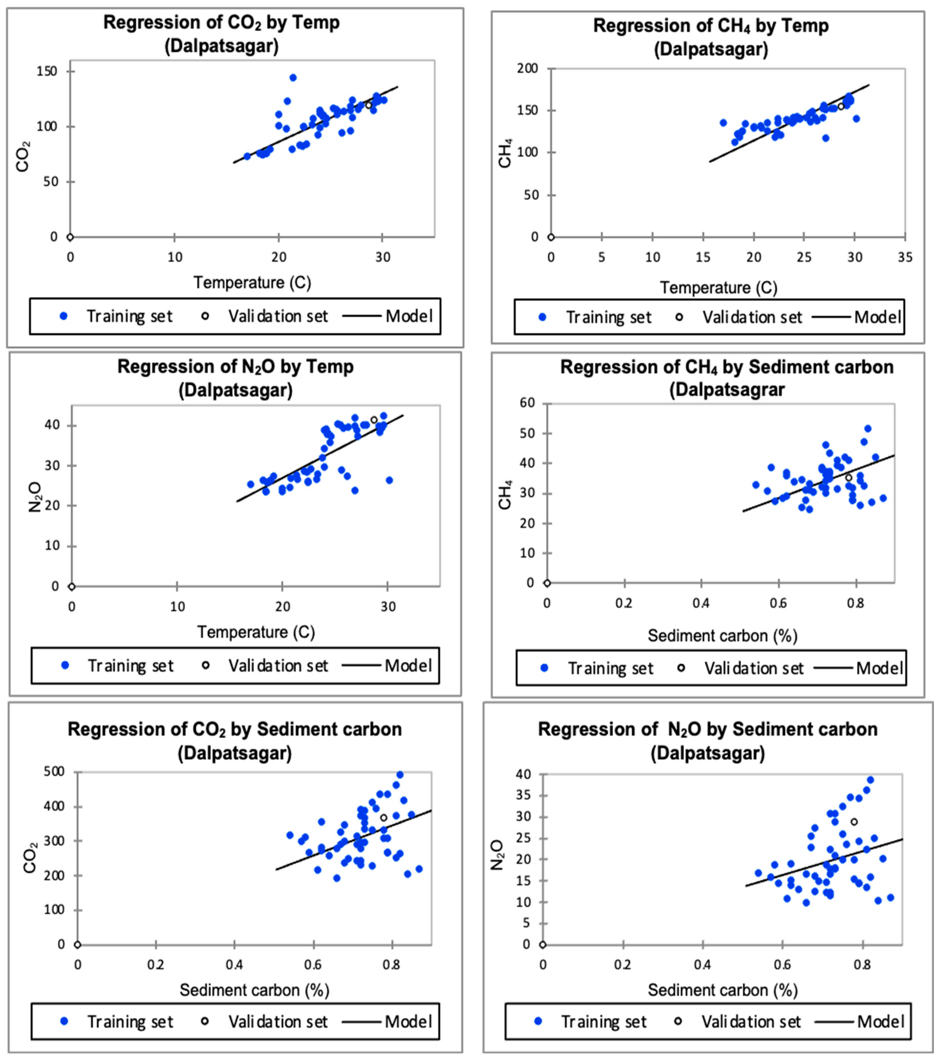
3.1. Dalpatsagar Water Body

3.1.1. Greenhouse Gases Influenced by Temperature

The Dalpatsagar water body is deep and nutrient-rich, and is regularly used for aquatic and human activities. The temperature difference between winter and hot summer is more than 10 °C, leading to a drastic change in GHG (CH₄, CO₂, and N₂O) emissions throughout the year. Methane was observed to be highest (167.24 mg m⁻² h⁻¹) at 29.4 °C during a standard meteorological week (21 May to 27 May); when the temperature was in the range of 17.0 °C to 18.0 °C, the methane released was almost 125 to 130 mg m⁻² h⁻¹, which showed that the temperature was significantly elevated by 2 to 3 °C when January and February demonstrated a rapid change in CH₄ levels. Higher temperatures were recorded from April to the first fortnight of June owing to high sunshine hours and rainless periods. Even the Dalpatsagar water body shrank and had a higher concentration of decomposed materials, and the column of the water body was also reduced, which helped in the rapid penetration of sun rays. However, in March (12th to 25th SMW), methane had fewer emissions owing to slightly less disturbance of the water body and less sewage entry, although methane emissions increased on sunny days until they reached the highest peak.

The period from the beginning of January to the first week of February showed a lower rate of CO₂ emissions than the rest of the month because the mild temperature did not influence more emissions, but the rate was slightly higher during the rest of February, declining slightly in March from the slightly lowered temperature (up to 17 °C). The temperature shifted from 17 °C to an upward emission rate of more than 35 mg m⁻² h⁻¹. As the temperature increased during the first half of June, CO₂ emissions peaked at 128.15 mg m⁻² h⁻¹. Furthermore, the decreasing trend of the temperature also decreased the emission of CO₂ when the emission of CO₂ was lower, and a similar pattern of release was observed at normal temperatures up to 30 °C. A sudden increase in CO₂ emissions (124.25 to 144.84 mg m⁻² h⁻¹ at 12 to 25 °C) occurred within two weeks. November and December were the coolest months. Nitrous oxide (N₂O) fluctuated in two major phases (i.e., higher and lower levels of emission), which were distinct in the observations recorded. From January to March, the N₂O emissions were maintained, ranging from 5 to 8 mg m⁻² h⁻¹, with a higher rate of emission (29.11 mg m⁻² h⁻¹) during the 8th standard meteorological week, which was slightly higher than the phase of lower emissions. From March onward, emissions of N₂O were higher till 25 August with a pace of 37 to 43 mg m⁻² h⁻¹, and later, N₂O declined from 24 September onward with a lower emission rate of 23.60 mg m⁻² h⁻¹.

3.1.2. Greenhouse Gases Influenced by Sediment Carbon

Sediment carbon contains a significant amount of methanogenesis materials, CO_2, and N₂O, which directly influence the emissions studied in water bodies by monitoring year-round observations. Dalpatsagar is rich in sediment carbon because of the long-term storage of sewage in large areas. Another reason for detritus deposition is aquatic flora, which is more than 50 cm thick at the bottom of Dalpatsagar. The emission of methane ranged from 24.59 to 51.72 mg m⁻² h⁻¹ during the 44th standard meteorological week (SMW). Monthly changes in sediment carbon caused drastic changes in the level of CH₄ emissions from benthic sediments. The sediment carbon that fell between 0.75 and 0.82 percent had 40 ± 5 mg m⁻² h⁻¹ carbon emissions, and the emission rate ranged 35 to 40 mg m⁻² h⁻¹, which showed an increase under anaerobic conditions that changed the emission of methane. A distinct increasing rate was noticed in April and May, when a distinctly higher rate of methane emissions was apparent during monitoring. Otherwise, a mixed trend of varying sediment carbon changed the rate of methane emissions. Spontaneous changes in sediment carbon were also monitored during the 16th, 29th, 30th, 34th, 38th, 43rd, and 44th standard meteorological weeks; from November onward, the sediment carbon levels decreased due to the lowered temperature. Carbon dioxide emissions ranged from 192 to 490 mg m⁻² h⁻¹ at 0.66, and 0.82% sediment carbon was noticed during monitoring. In January, carbon dioxide emissions increased or decreased further as sediment carbon fluctuated with the morphological condition of the Dalpatsagar water body. Sediment carbon levels greater than 300 mg m⁻² h⁻¹ were measured at 0.72, 0.73, 0.72, 0.70, 0.73, 0.78, 0.72, 0.76 and 0.81 percent and CO₂ emissions were recorded as 389, 366, 372, 351, 388, 365, 376, 33, 354 and 371 mg m⁻² h⁻¹, respectively. The emission of N₂O is a major threat among GHGs, and the monitoring of emissions was observed from the Dalpatsagar water body, with an emission rate range from low to high (20.38 to 31.51 mg m⁻² h⁻¹). A higher rate of N₂O emissions was recorded at 32.36 mg m⁻² h⁻¹ with 0.75 percent sediment carbon CH₄ and CO₂, whereas N₂O varied slightly from the validation set due to few observations at the Dalpatsagar water body. Sediment carbon also showed a sparse pattern of CH₄ and CO₂ as well as over-increased and decreased levels of carbon (Figure 5).

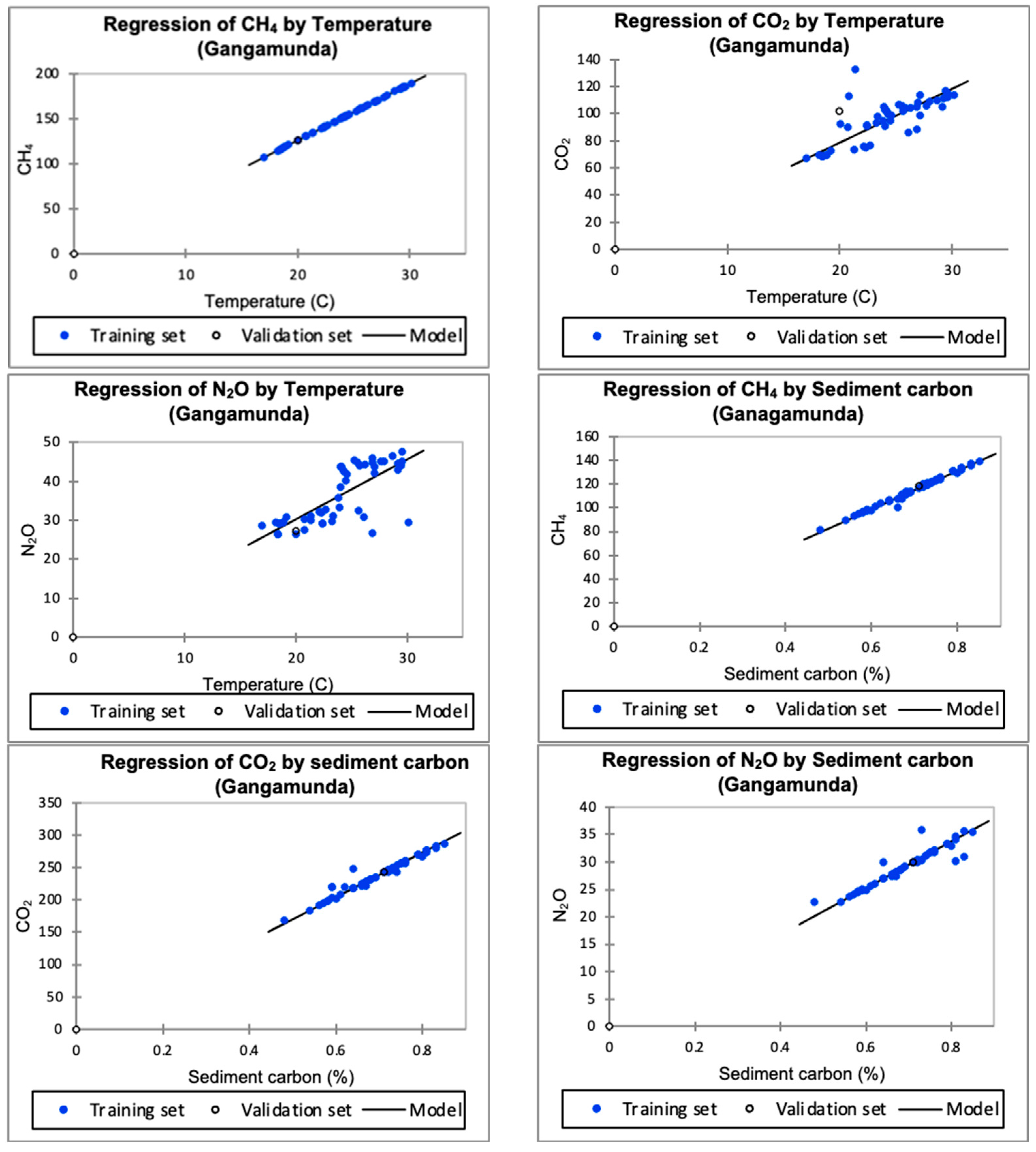
3.2. Gangamunda Water Body

3.2.1. Greenhouse Gases Influenced by Temperature

Jagdalpur city is known for water harvesting practices since ancient times owing to its topography and rainfall variability; when available, surface water from the Gangamunda water body is used throughout the year as storage water for people’s use. Its water quality and GHG emissions change drastically throughout the year because anthropogenic activity is very common. Temperature and sediment carbon influence the emissions of CH₄, CO₂, and N₂O from water bodies. However, the Gangamunda water body was assumed to be an older water body among the water bodies selected for this study. Methane emissions from Gangamunda were dynamic in response to temperature fluctuations, and the rate of emission was widely governed by temperature increases and declines throughout the year. In the beginning months of this study, methane emissions were lower than those of the other months (110.21 to 118.47 mg m⁻² h⁻¹) because the temperature range was within 17.0 to 18.86 °C; higher temperatures raised the emission rates (113.50 to 142.60 mg m⁻² h⁻¹). The increment was higher, from 22 °C onward, and reached its highest level (185.3 mg m⁻² h⁻¹) at 29.61 °C, which was recorded from the 16th SWM (16 April to 22 April) to 25th SMW (18 June to 24 June) under slightly higher temperature.

Carbon dioxide levels were greatly influenced by temperature variations in January, when the lowest level of CO₂ loss was observed. The levels were accelerated by the rising temperatures after January; the emission of CO₂ was 10 mg m⁻² h⁻¹ higher than that in earlier months (2–3 °C more). A light shower of 80 mm in March reduced the temperature, resulting in the emission of CO₂, which gained momentum from April onward. Emissions reached their highest peak of 113.72 mg m⁻² h⁻¹, which was later maintained at a slightly lower level until August. They declined more sharply in September and increased in November along with the temperature. Otherwise, emissions remained static until December. Sewage discharged by industries that cover a large volume of organic materials tends to produce GHG emissions. With the discharge of sewage into water bodies, the release of CH₄ and N₂O in the water is indirectly affected.

Nitrous oxide is another GHG among the gases responsible for climate change and is mostly governed by the limnological dynamics of the water body. Gangamunda is a confined water body that is changed by the shuffling of water either through natural outflow or anthropogenic activities that are common to the water body. The N₂O fluctuation rate increased from 26.0 to 47.68 mg m⁻² h⁻¹ over the year and from April to the last week of August and into September, quickly reducing the level of emissions to almost 10.0 mg m⁻² h⁻¹. The change in the emission of nitrous oxide was synchronized more with a temperature range between 25 °C and 30 °C; hence, the emission rate was highly influenced by the sharp change in temperature.

3.2.2. Greenhouse Gases Influenced by Sediment Carbon

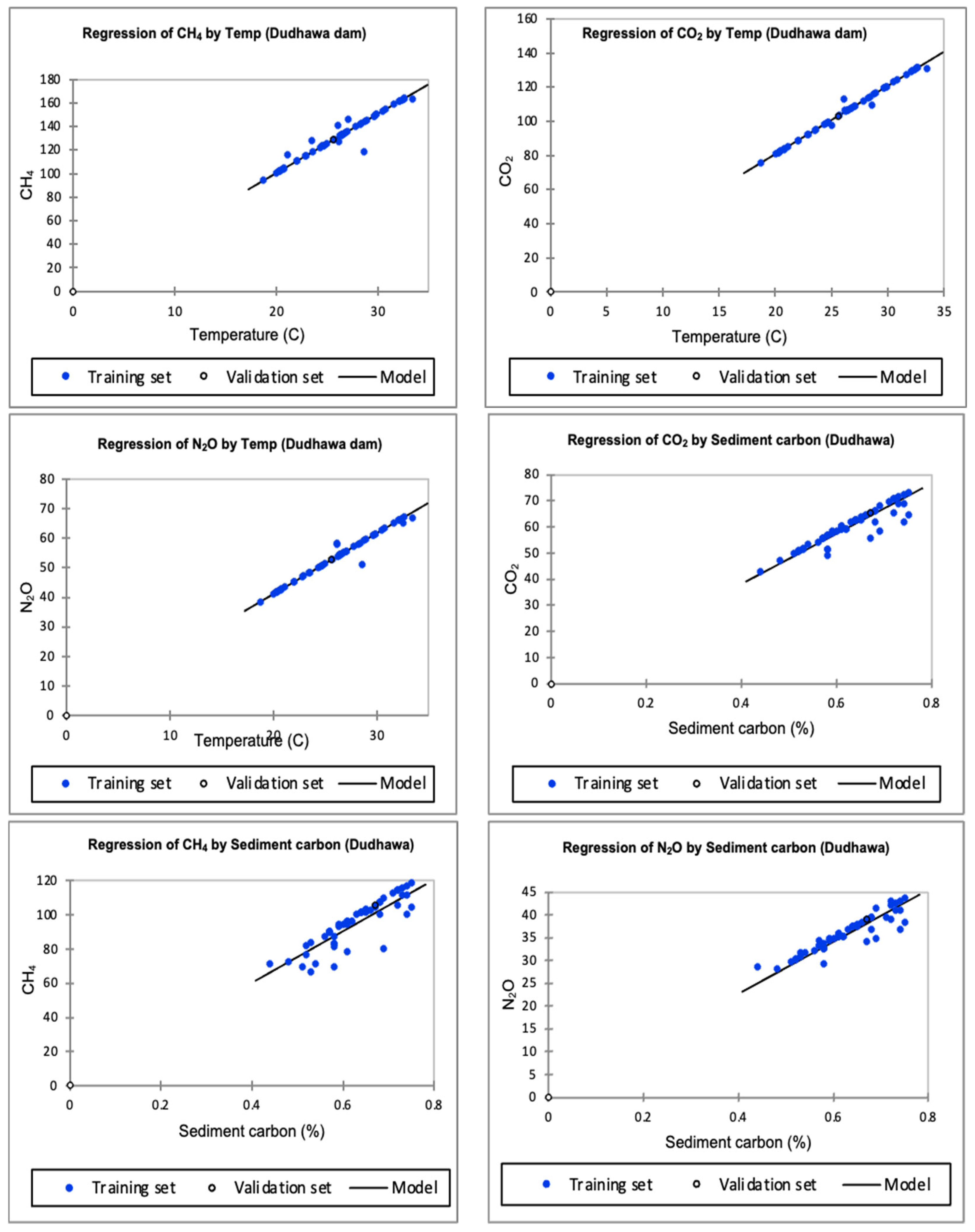
The bottom of Gangamunda had varied levels of sediment carbon ranging from 0.48 to 0.85%, showing a wider range of carbon deposited into the bottom via the process of the decomposition of the organic waste that remained in Gangamunda, which was influenced positively by the variation in sediment carbon throughout the year. The emission rate was higher with higher (>0.50%) sediment carbon CH₄, CO₂, and N₂O emissions. Hence, methane emissions were very slow with less sediment carbon, but they increased more intensively as the carbon level increased. As sediment carbon ranged from 0.70 to 0.75, the CH₄ emissions were more than 120 mg m⁻² h⁻¹, and the 125.61 mg m⁻² h⁻¹ of methane emissions were accelerated by 0.76% sediment carbon. On the other hand, when sediment carbon was 0.80% or more, the emission rate was 138.84 mg m⁻² h⁻¹ during the 46th standard meteorological week (12 November to 18 November). Below 0.60% sediment carbon, the emission rate was less than 100.0 mg m⁻² h⁻¹, which was accelerated until it rose above the limit (0.70%) of sediment carbon and later increments were sluggish.

Carbon dioxide (CO₂) emissions were influenced by sediment carbon more effectively in the Gangamunda aquatic system. Due to the shallow depth of its water, the sediment carbon fluctuated significantly over the study months, even changing the CO₂ emission level. It was observed that less sediment carbon (<0.65%) released nearly 220 mg m⁻² h⁻¹ CO₂, and an increase of more than 0.60% in sediment carbon drastically increased the emission, which was almost 20–25 mg m⁻² h⁻¹ during February. More CO₂ emissions coincided with a range of 0.70 to 0.75% sediment carbon curbing of 256.50 mg m⁻² h⁻¹ during March, which may have been due to the increased decomposition rate. A prominent level of emission was noticed from mid-March to mid-April, whereas a moderate level of CO₂ emission (230 to 246.24 mg m⁻² h⁻¹) was observed later in October. More than 270.0 mg m⁻² h⁻¹ emission was observed with higher sediment carbon (0.79 to 0.83%).

Nitrous oxide (N₂O) was more influenced by sediment carbon, with 2 to 30 mg m⁻² h⁻¹ recorded in the initial months of January and February. With the increasing sediment carbon, N₂O was enhanced between 30.0 and 32.0 mg m⁻² h⁻¹ because of drastic trophic level changes in the denitrification and nitrification processes in the varied depth of the water body, which directly correlated with sediment carbon levels. Temperature somehow controlled the emission rate of CH₄ linearly; however, CO₂ and N₂O were found in a scattered pattern during the temperature fluctuations. Sediment carbon exhibited a similar trend in response to CH₄, CO₂, and N₂O in the linear model of the Gangamunda water body (Figure 6).

3.3. In Dudhawa Dam

3.3.1. Greenhouse Gases Influenced by Temperature

The Dudhawa Dam is a manmade reservoir constructed for irrigation purposes that recycles water and changes the emissions of CH₄, CO₂, and N₂O by replacing water from the dam. The quality of the water body is greatly influenced by seasonal temperatures and sediment carbon. The initial temperature, up to 20 °C, affected CH₄ emissions by approximately 97.24 to 104.52 mg m⁻² h⁻¹ as the temperature shifted from 19 to 20 °C. Furthermore, the temperature’s shift from 20 °C to 24 °C raised the emission rate to about 20 mg m⁻² h⁻¹, which was observed later from the 43rd SMW until December. The change in the emissions was more significant at higher temperatures. In warmer months, i.e., mid-March to June, the temperature rose to over 30 °C and increased CH₄ to 164.05 mg m⁻² h⁻¹ due to the greater activity of carbon in the bottom-enhanced CH₄ emissions. The lowest CO₂ emission was observed in this study’s initial month, as rising temperatures from 10 °C to 12 °C increased the carbon dioxide emissions, which still remained below 83.74 mg m⁻² h⁻¹. However, a considerable increment was noticed with April (14th SMW) onward, ranging from 120.39 mg m⁻² h⁻¹ to 130.72 mg m⁻² h⁻¹, and was maintained till the 25th SMW. The higher water column of the Dudhawa Dam and the disturbance of the water body influenced the emission of N₂O, and the highest emission was recorded as 66.86 mg m⁻² h⁻¹ on the 23rd SMW (4 to 10 June), whereas the lowest emission (39.84 mg m⁻² h⁻¹) was recorded in January.

3.3.2. Greenhouse Gases Influenced by Sediment Carbon

The weekly monitoring of sediment carbon varied with the changing months and ultimately revealed that the emission levels of the GHGs were more noticeable in the Dudhawa Dam. A higher magnitude of fluctuation was observed in CH₄ than in CO₂ and N₂O, but both CO₂ and N₂O were considered as direct and indirect changes under the influence of sediment carbon. However, the lowest (0.44%) and highest (0.74%) sediment carbon levels had almost a 0.30% difference in all observations, triggering emission differences in GHGs.

The CH₄ emission was about 91.54 mg m⁻² h⁻¹ and increased further in 1st week of March, ranging from 101.40 to 107.03 mg m⁻² h⁻¹, and a lower quantity of sediment was also influenced by the lower emissions. Moreover, the variation in sediment carbon was mostly the same, owing to the lower decomposition level. The sediment decomposition rate was similar throughout the year because of less variation in the carbon level. Therefore, methane emissions fluctuated slightly because of the other associated factors that were a little varied. Carbon dioxide (CO₂) emissions were higher from March to April when the temperature rose up to 60–66 mg m⁻² h⁻¹ over the exiting pattern under higher sediment carbon, which was similar to the emission levels from mid-July to late December; otherwise, the remaining period’s emission was almost 50.03 mg m⁻² h⁻¹ while still <60.0 mg m⁻² h⁻¹. The nitrous oxide (N₂O) emissions of the Dudhawa Dam are exhibited according to sediment carbon, and the highest N₂O emission was recorded as 43.02 mg m⁻² h⁻¹ under a sediment carbon level of 0.74% in the last week of December, whereas the lowest level was 28.48 mg m⁻² h⁻¹ at 0.44% in the 21st SMW (21 May to 27 May). A similar trend was observed throughout the year with slight variations in emissions, but a higher rate of N₂O emission was observed from mid-November to December.

The precise model showed a conglomerated linear representation of temperature and sediment carbon with CH₄, CO_2, and N₂O emissions. Regarding temperature, this factor governed the linear pattern. When the regression line was generated from the model development of the Dudhawa Dam, the model showed a linear increase in CH₄, CO₂, and N₂O in response to the temperature of the water body studied. Methane showed little variation in the training set over the validation set of the model as compared with CO₂ and N₂O. In contrast, sediment carbon was assumed to be an independent factor which significantly influenced gas emissions. Among these gases, CH₄ emissions were highly influenced by sediment carbon as compared with those of CO₂ and N₂O, an almost linear model with a training set (Figure 7).

3.4. Global Warming Potential of Water Bodies

The Dalpatsagar water body released higher rates of CO₂, CH₄, and N₂O, which further accumulated as high global-warming potential and carbon equivalent emissions to the environment, which were significantly higher than the Dudhawa Dam’s emissions but on par with the Gangamunda water body’s emissions. However, Gangamunda had a minimum emission of CO₂, which was not found significant, unlike the Dalpatsagar water body’s emissions (

Table 3. Emissions of CO₂, N₂O, CH₄ and the global warming potentials of the water bodies.

Water Body	CO2 (mg m−2 h−1)	N2O (mg m−2 h−1)	CH4 (mg m−2 h−1)	Global Warming Potential (mg m−2 h−1)	Carbon Equ. Emission (mg m−2 h−1)
Dalpatsagar	59.48 **	36.92 **	90.76 **	13,410 **	3657 **
Gangamunda	47.06	34.90 **	85.03 **	12,658 **	3452 **
Dudhawa Dam	40.48	23.38	62.31	8597	2344

Note: ** = significant at p < 0.01.

). The essential characteristics of the dam as a larger water body and irrigation dam frequently used for storing recycled rainwater from Dudhawa are the reasons for the lower rate of emission; even at its lowest depth, it was higher than the rest of the two water bodies.

4. Discussion

4.1. Dalpatsagar Water Body

4.1.1. Greenhouse Gases Affected by Temperature

The results suggest that there is a positive relationship between concentrations of GHGs and temperature as well as the sediment contents of the Dalpatsagar water body. Higher temperatures lead to decreased concentrations of dissolved oxygen and increased levels of dissolved CO₂ levels that enhance CH₄ production, especially in eutrophic systems [2,9,15]. The elevated temperature lowers the dissolved-oxygen levels, which in turn encourages conditions conducive to methanogenesis; moreover, the variation in the methane output is increased during the warmer months [24]. These processes show how sediment carbon forms and interacts with temperature and oxygen to release gases, including methane, iron, and other phenomena contributing to GW. The high values noted during the peak production rate of methane are attributed to the sediment’s temperature influences, particularly the microbial effects noticeable at 29.4 °C; this is supported by other studies on emission variations related to temperature fluctuations. Similarly, methane emissions also decreased with lower temperatures, thereby implying a temperature-dependent emission circulation. Indeed, CO₂ emissions were highest in warmer months due to the increasing microbial actions that favor the respiration of organic matter. The increase in nitrous oxide N₂O emissions during higher temperatures are attributed to increased nitrification and denitrification, which are regulated by sediment nutrients and organic matter content.

4.1.2. Greenhouse Gases Affected by Sediment Carbon

This study shows how the quantified sediment carbon is fundamental to GHG emissions on account of its influence on microbial decomposition. Furthermore, the 50-cm detritus layer in Dalpatsagar demonstrates the extension of the organic matter deposition, which supports more methanogenesis and CO₂ liberation [1,25]. Data analysis demonstrated that changes in the sediment carbon concentration were coordinated with changes in methane and CO₂ production, with greater production rates under anaerobic conditions in warmer months. These data therefore stress the role of sediment content and microbial processes in controlling GHG dynamics. A sudden spurt in methane emissions was observed during April and May when the water temperature was increasing and the water volume was decreasing, which increased light penetration and led to more efficient decomposition of the sediment. Concurrently, CO₂ emissions also followed a seasonal trend, reaching their highest level at 490 mg m⁻² h⁻¹ when sediment carbon was also at its highest level (0.66–0.82%). Nitrous oxide emissions also increased with depth, displaying a maximum value of 32.36 mg m⁻² h⁻¹, suggesting that nitrogen cycling influences the sediment processes.

4.2. Greenhouse Gases: Temperature and Sediment in the Gangamunda Water Body

The Gangamunda water body revealed a temporal change in GHG flux under rising temperatures, with methane emissions varying between 110.21 ± 22.6 and 185.3 ± 28.1 mg m⁻² h⁻¹. Notably, the emission rate was augmented when the temperature surpassed an average of 22 °C, as the activities of microbes and the decomposition of OM were further amplified. Rainfall events intensified CO₂ emissions in several ways by replacing the pockets of soil and air charged with CO_2, which released the gas into the ambient air in abundance. The emission rates of nitrous oxide in Gangamunda were highly influenced by temperature and had the highest release rate of 47.68 mg m⁻² h⁻¹ in the period between April and August. This pattern suggests that trophic interactions and processes of denitrification control N₂O emissions [26]. Higher sediment carbon content (>0.75%) was associated with elevated CH₄ and CO₂ emissions, highlighting the role played by sediment organic matter in maintaining metabolic activity.

4.3. Sediment Carbon in the Gangamunda Water Body

Fluctuations in sediment carbon content within the range of 0.48–0.85% were key in influencing the emissions of GHGs in Gangamunda. Methane emissions increased with the increase in sediment carbon content to above 0.70% and a maximum of 3.3 mg m⁻² h⁻¹ at 0.80% sediment carbon. Similar trends were observed for the CO₂ emissions, which, like the CH₄ emissions, were found to be above 270 mg m⁻² h⁻¹ during periods of C sediment carbon, high microbial decomposition, and high rate of organic matter turnover. N₂O emissions had a positive correlation with sediment carbon maximizing at 32.0 mg m⁻² h⁻¹. These observations readily demonstrate how temperature and sediment characteristics act together to modulate the effluxes of GHGs, especially in shallow water bodies with high loading of organic matter.

4.4. Greenhouse Gases Influenced by Temperature and Sediment at Dudhawa Dam

The overall GHG emissions from the Dudhawa Dam were also considerably lower than those from Dalpatsagar and Gangamunda because the Dudhawa Dam is wider and has a greater water column. Methane emissions, in general, ranged from 97.24 to 164.05 mg m⁻² h⁻¹, and the highest emission rates were observed during the warmer months, from March–June. There are clear trends in both microbial activity and sediment decomposition, in response to temperature changes across the study area, especially where organic loading favored methanogenic conditions. The flux density of carbon dioxide depicts an upward trend with increasing temperature and the highest recorded value was 130.72 mg m⁻² h⁻¹ during April. Altogether, the obtained results show that N₂O emissions were characterized by a quite different pattern: the highest value of 66.86 mg m⁻² h⁻¹ was observed in June in connection with the rise of the N inputs and the denitrification activity. These findings reveal that temperature, sediment type, and hydrological fluctuation play key roles in determining the level of GHG emissions.

The C content of sediments (0.44–0.74%) in the Dudhawa Dam were characteristic and showed relatively constant C parameters, indicating the engagement of sediments in the decomposition of organic matter and nutrient cycling. Total methane emission rates rose with sediment carbon levels and reached their peak of 107.03 mg m⁻² h⁻¹ with high organic carbon content values. In a similar pattern, seasonality was observed in the CO₂ emissions, with heightened values relative to microbial activity. Fluxes of N₂O reached 43.02 mg m⁻² h⁻¹ during the wet season under conditions of higher sediment-carbon characteristics. These results suggest that sediment and microbial activities play important parts in controlling the release of gases that cause the greenhouse effect, especially in large water bodies where hydrological conditions remain more or less consistent.

4.5. Water Bodies’ Global Warming Potential

The present study depicts the global warming potentials of the studied water bodies and their varying contributions to emissions of atmospheric GHGs. Our results show that Dalpatsagar has the highest GWP of 13,410 mg m⁻² h⁻¹, Gangamunda has a GWP of 12,658 mg m⁻² h⁻¹, and Dudhawa Dam has a GWP of 8597 mg m⁻² h⁻¹. These variations demonstrate the impacts of temperature, sediment type, and runoff on the control of GHG emissions. The higher emissions of Dalpatsagar were due to nutrient-rich sediments and more frequent anthropogenic inputs, while Gangamunda’s emissions were directly proportional to its sediment carbon and temperature. The Dudhawa Dam had lower emissions due to its larger surface area and deeper water column, in addition to the fact that the water flow through the dam is recycled periodically, thus decreasing the accumulation of organic matter and microorganisms.

This study highlights the significant role of small, dammed wetland systems in contributing to regional GHG emissions, emphasizing their relevance to global carbon budgeting, particularly within tropical regions. The observed high CH₄ and CO₂ fluxes, influenced by temperature variations, suggest that climate change may intensify biogeochemical processes in these ecosystems. These results support the need for incorporating small reservoirs in both national and international GHG inventories [27,28]. Additionally, the correlation between water quality degradation and heightened emissions points to potential public health risks, underscoring the importance of integrated water management and climate adaptation policies. However, this study is constrained by a limited short-term temporal scale, restricted spatial coverage, and insufficient mechanistic understanding of the emission drivers behind GHG emissions [29]. The absence of control sites and insufficient extrapolation to annual or global scales further restricts its broader applicability. To address these gaps, future research should prioritize long-term, multi-seasonal monitoring, the inclusion of comparative control systems, and the development of mechanistic and predictive models [30]. Additionally, articulating targeted mitigation strategies (e.g., improved wetland management, aeration interventions, and nutrient load reductions) would enhance the practical relevance of the findings for policy design and implementation [31].

This study highlights the influence of seasonal temperature fluctuations and sediment OC on GHG emissions from three freshwater bodies in Central India. However, three key limitations have been highlighted. First, the temporal resolution may not fully capture the interannual variability [32]. Second, the spatial scope is limited to three water bodies, which may cause potentially restrictive generalization across heterogeneous freshwater environments [33]. Third, this study focuses on surface sediment properties without considering vertical sediment profiles or porewater chemistry that may harbor significant biogeochemical gradients that influence gas production [34]. Additionally, the absence of a microbial community analysis limits our understanding of the microbial mechanisms underlying GHG emissions [34]. Hydrological factors like water level fluctuations, sediment resuspension, and aquatic vegetation dynamics were also not explicitly considered [35]. In light of these, future research should integrate high-frequency, year-round monitoring to capture temporal variability more comprehensively and combine microbial, genomic, and sediment core analyses to elucidate key drivers of GHG dynamics [36]. Process-based modeling approaches (e.g., DNDC, SWAT-GHG) can help simulate emissions under various climate and land-use scenarios [37]. These findings also call for the inclusion of freshwater GHG fluxes in national inventories and the development of adaptive, climate-resilient water resource management strategies [38]. Strengthening ecosystem-scale mitigation efforts through stakeholder engagement and targeted interventions will be crucial for protecting water quality and reducing health risks caused by rising CO₂ levels and global warming.

5. Conclusions

This study reveals that seasonal temperature changes and sediment organic carbon content significantly influence CH₄, CO₂, and N₂O emissions across three freshwater bodies: the Dalpatsagar, Gangamunda, and Dudhawa dams. Methane emissions were highest in Dalpatsagar (167.24 mg m⁻² h⁻¹) during warmer months (~29.4 °C), while Gangamunda showed moderate emissions (125–130 mg m⁻² h⁻¹) even at lower temperatures, pointing to localized biogeochemical influences. CO₂ fluxes correlated with rising temperatures and higher sediment carbon, reaching up to 490 mg m⁻² h⁻¹ in Dalpatsagar. The Dudhawa Dam, despite similar thermal profiles, had lower CH₄ but higher N₂O emissions (66.86 mg m⁻² h⁻¹) in the early summer, which declined with cooling temperatures, highlighting the sensitivity of nitrogen cycling to temperature. These findings underscore the critical roles of benthic processes and environmental conditions in regulating greenhouse gas dynamics in freshwater ecosystems. As climate variability increases, these emissions contribute meaningfully to regional carbon and nitrogen budgets, with broader implications for ecosystem health and public well-being. Targeted, climate-resilient water resource management is essential to mitigate risks, protect water quality, and ensure the sustainable use of these vulnerable aquatic systems.

References

1. Peacock, M.; Audet, J.; Jordan, S.; Smeds, J.; Wallin, M.B. Greenhouse gas emissions from urban ponds are driven by nutrient status and hydrology. Ecosphere 2019, 10, e02643. [Google Scholar] [CrossRef]
2. Jensen, S.; Leavitt, P.R.; Baulch, H.M.; Badiou, P.; Cordeiro, M.R.C.; Webb, J.R. Differential Controls of Greenhouse Gas (CO2, CH4, and N2O) Concentrations in Natural and Constructed Agricultural Waterbodies on the Northern Great Plains. J. Geophys. Res. Biogeosci. 2023, 128, e2022JG007261. [Google Scholar] [CrossRef]
3. Yang, P. Fluxes of carbon dioxide and methane across the water-atmosphere interface of aquaculture shrimp ponds in two subtropical estuaries: The effect of temperature, substrate, salinity and nitrate. Sci. Total Environ. 2018, 635, 1025–1035. [Google Scholar] [CrossRef] [PubMed]
4. IPCC. Summary for Policymakers. In Climate Change 2013: The Physical Science Basis Contribution of Working Group I to the Fifth Assessment Report of the Intergovernmental Panel on Climate Change; Stocker, T.F., Qin, D., Plattner, G.-K., Tignor, M., Allen, S.K., Boschung, J., Nauels, A., Xia, Y., Bex, V., Midgley, P.M., Eds.; Cambridge University Press: Cambridge, UK; New York, NY, USA, 2013; 1535p. [Google Scholar] [CrossRef]
5. IPCC. Climate Change (2014). Fifth Assessment Synthesis Report (Longer Report) of Intergovernmental Panel on Climate Change; Cambridge University Press: Cambridge, UK; New York, NY, USA, 2014. [Google Scholar]
6. Olefeldt, D. Net carbon accumulation of a high-latitude permafrost palsa mire similar to permafrost-free peatlands. Geophys. Res. Lett. 2012, 39, L03501. [Google Scholar] [CrossRef]
7. ICAR. Handbook of Fisheries and Aquaculture; ICAR: New Delhi, India, 2011. [Google Scholar]
8. Dusek, J.; Darenova, E.; Pavelka, M.; Marek, M.V. Methane and Carbon Dioxide Release from Wetland Ecosystems. In Climate Change and Soil Interactions; Elsevier: Amsterdam, The Netherlands, 2020; pp. 509–553. [Google Scholar]
9. Deemer, B.R.; Harrison, J.A.; Li, S.; Beaulieu, J.J.; Delsontro, T.; Barros, N.; Bezerra-Neto, J.F.; Powers, S.M.; Dos Santos, M.A.; Vonk, J.A. Greenhouse gas emissions from reservoir water surfaces: A new global synthesis. BioScience 2016, 66, 949–964. [Google Scholar] [CrossRef]
10. Rosentreter, J.A.; Borges, A.V.; Deemer, B.R.; Holgerson, M.A.; Liu, S.; Song, C.; Melack, J.; Raymond, P.A.; Duarte, C.M.; Allen, G.H.; et al. Half of Global Methane Emissions Come from Highly Variable Aquatic Ecosystem Sources. Nat. Geosci. 2021, 14, 225–230. [Google Scholar] [CrossRef]
11. Bastviken, D.; Cole, J.J.; Pace, M.; Tranvik, L. Methane emissions from lakes: Dependence of lake characteristics, two regional assessments, and a global estimate. Glob. Biogeochem. Cycles 2004, 18, GB4009. [Google Scholar] [CrossRef]
12. Kumar, S.; Bijalwan, A. Comparison of Carbon Sequestration Potential of Quercus leucotrichophora Based Agroforestry Systems and Natural Forest in Central Himalaya, India. Water Air Soil Pollut. 2021, 232, 350. [Google Scholar] [CrossRef]
13. Alin, S.R.; Johnson, T.R. Physical controls on carbon dioxide transfer velocity and flux in low-gradient river systems and implications for regional carbon budgets. J. Geophys. Res. 2007, 116, G01009. [Google Scholar] [CrossRef]
14. Wei, D.; Tarchen, T.; Dai, D.; Wang, Y.; Wang, Y. Revisiting the role of CH4 emissions from alpine wetlands on the Tibetan Plateau: Evidence from two in situ measurements at 4758 and 4320 m above sea level. J. Geophys. Res. Biogeosci. 2015, 120, 1741–1750. [Google Scholar] [CrossRef]
15. Bevelhimer, M.; Stewart, A.; Fortner, A.; Phillips, J.; Mosher, J. CO2 is Dominant Greenhouse Gas Emitted from Six Hydropower Reservoirs in Southeastern United States during Peak Summer Emissions. Water 2016, 8, 15. [Google Scholar] [CrossRef]
16. Adams, D.D. Diffuse Flux of Greenhouse Gases—Methane and Carbon Dioxide—At the Sediment-Water Interface of Some Lakes and Reservoirs of the World. In Greenhouse Gas Emissions—Fluxes and Processes; Garneau, M., Tremblay, A., Roehm, C., Varfalvy, L., Eds.; Springer: Berlin/Heidelberg, Germany, 2005; pp. 129–153. [Google Scholar]
17. Pradhan, A.; Chandrakar, T.; Nag, S.K.; Dixit, A.; Mukherjee, S.C. Crop planning based on rainfall variability for Bastar region of Chhattisgarh. India J. Agrometeorol. 2017, 22, 509–517. [Google Scholar] [CrossRef]
18. Hutchinson, G.L.; Mosier, A.R. Improved soil cover method for field measurement of nitrous oxide fluxes. Soil Sci. Soc. Am. J. 1981, 45, 311–316. [Google Scholar] [CrossRef]
19. Liu, C.; Holst, J.; Brueggemann, N.; Butterbach-Bahl, K.; Yao, Z.; Yue, J.; Han, S.; Han, X.; Zheng, X. Winter-grazing reduces methane uptake by soils of a typical semi-arid steppe in Inner Mongolia, China. Atmos. Environ. 2016, 145, 105–113. [Google Scholar] [CrossRef]
20. Yvon-Durocher, G.; Allen, A.P.; Bastviken, D.; Conrad, R.; Gudasz, C.; St-Pierre, A.; Thanh-Duc, N.; del Giorgio, P.A. Methane fluxes show consistent temperature dependence across microbial to ecosystem scales. Nature 2014, 507, 488–491. [Google Scholar] [CrossRef]
21. Pathak, H.; Upadhyay, R.C.; Muralidhar, M.; Bhattacharyya, P.; Venkateswarlu, B. Measurement of Greenhouse Gas Emission from Crop, Livestock and Aquaculture; Indian Agricultural Research Institute: New Delhi, India, 2013; p. 101. [Google Scholar]
22. Lal, R. Soil carbon sequestration in India. Clim. Change 2004, 65, 277–296. [Google Scholar] [CrossRef]
23. DelSontro, T.; Beaulieu, J.J.; Downing, J.A. Greenhouse Gas Emissions from Lakes and Impoundments: Upscaling in the Face of Global Change. Limnol. Oceanogr. Lett. 2018, 3, 64–75. [Google Scholar] [CrossRef]
24. Lamers, P.M.; van Roozendaal, M.E.; Roelofs, G.M. Acidification of freshwater wetlands: Combined effects of non- airborne sulfur pollution and desiccation. Water Air Soil Pollut. 1998, 105, 95–106. [Google Scholar] [CrossRef]
25. Rawat, S.; Khanduri, V.P.; Singh, B.; Riyal, M.K.; Thakur, T.K.; Kumar, M.; Cabral-Pinto, M.M. Variation in carbon stock and soil properties in different Quercus leucotrichophora forests of Garhwal Himalaya. CATENA 2022, 213, 106210. [Google Scholar] [CrossRef]
26. Vizza, C.; West, W.E.; Jones, S.E.; Hart, J.A.; Lamberti, G.A. Regulators of coastal wetland methane production and responses to simulated global change. Biogeosciences 2017, 14, 431–446. [Google Scholar] [CrossRef]
27. Cheng, S.; Kumar, A.; Lan, G.; Zhang, W.; Yu, Z.; Zhang, S.; Yu, Z.-G.; Yao, M.; Lin, J. Thermal sensitivity and rising greenhouse gas emissions in riparian zone soils: Implications for ecosystem carbon dynamics. J. Env. Manag. 2025, 381, 125194. [Google Scholar] [CrossRef] [PubMed]
28. Mondal, B.; Bauddh, K.; Kumar, A.; Bordoloi, N. India’s Contribution to Greenhouse Gas Emission from Freshwater Ecosystems: A Comprehensive Review. Water 2022, 14, 2965. [Google Scholar] [CrossRef]
29. Malyan, S.K.; Singh, O.; Kumar, A.; Anand, G.; Singh, R.; Singh, S.; Yu, Z.; Kumar, J.; Fagodiya, R.K.; Kumar, A. Greenhouse Gases Trade-Off from Ponds: An Overview of Emission Process and Their Driving Factors. Water 2022, 14, 970. [Google Scholar] [CrossRef]
30. Zhao, Y.; Lin, J.; Cheng, S.; Wang, K.; Kumar, A.; Yu, Z.; Zhu, B. Linking soil dissolved organic matter characteristics and the temperature sensitivity of soil organic carbon decomposition in the riparian zone of the Three Gorges Reservoir. Ecol. Indic. 2023, 154, 110768. [Google Scholar] [CrossRef]
31. Upadhyay, P.; Prajapati, S.K.; Kumar, A. Impacts of riverine pollution on greenhouse gas emissions: A comprehensive review. Ecol. Indic. 2023, 154, 110649. [Google Scholar] [CrossRef]
32. Tranvik, L.J.; Downing, J.A.; Cotner, J.B.; Loiselle, S.A.; Striegl, R.G.; Ballatore, T.J.; Dillon, P.; Finlay, K.; Fortino, K.; Knoll, L.B.; et al. Lakes and reservoirs as regulators of carbon cycling and climate. Limnol. Oceanogr. 2009, 54, 2298–2314. [Google Scholar] [CrossRef]
33. Bastviken, D.; Tranvik, L.J.; Downing, J.A.; Crill, P.M.; Enrich-Prast, A. Freshwater methane emissions offset the continental carbon sink. Science 2011, 331, 50. [Google Scholar] [CrossRef] [PubMed]
34. Nazaries, L.; Murrell, J.C.; Millard, P.; Baggs, L.; Singh, B.K. Methane, microbes and models: Fundamental understanding of the soil methane cycle for future predictions. Environ. Microbiol. 2013, 15, 2395–2417. [Google Scholar] [CrossRef]
35. Beaulieu, J.J.; Tank, J.L.; Hamilton, S.K.; Wollheim, W.M.; Hall, R.O., Jr.; Mulholland, P.J.; Peterson, B.J.; Ashkenas, L.R.; Cooper, L.W.; Dahm, C.N.; et al. Nitrous oxide emission from denitrification in stream and river networks. Proc. Natl. Acad. Sci. USA 2019, 116, 9802–9807. [Google Scholar] [CrossRef]
36. Borges, A.V.; Darchambeau, F.; Teodoru, C.R.; Marwick, T.R.; Tamooh, F.; Geeraert, N.; Omengo, F.O.; Guérin, F.; Lambert, T.; Morana, C.; et al. Globally significant greenhouse-gas emissions from African inland waters. Nat. Geosci. 2018, 11, 637–642. [Google Scholar] [CrossRef]
37. IPCC. Sixth Assessment Report; Intergovernmental Panel on Climate Change: Geneva, Switzerland, 2021. [Google Scholar]
38. Bărbulescu, A. Modeling Greenhouse Gas Emissions from Agriculture. Atmosphere 2025, 16, 295. [Google Scholar] [CrossRef]
Figure 1. Base map and location map of the study area.
Water 17 01553 g001
Figure 2. Inlet and outlet georeferencing of selected water bodies: Site I.: Dudhawadam (water body), Site II.: Dalpatsagar, and Site III.: Gangamunda water body).
Water 17 01553 g002
Figure 3. (a) Rainfall and (b) temperature pattern of the study area.
Water 17 01553 g003aWater 17 01553 g003b
Figure 4. Digital elevation map of the study area.
Water 17 01553 g004
Figure 5. Regression model of the emission of GHGs influenced by the temperature and sediment of the Dalpatsagar wetland.
Water 17 01553 g005
Figure 6. Regression model of the emission of GHGs influenced by the temperature and sediment of the Gangamunda wetland.
Water 17 01553 g006
Figure 7. Regression model of the emissions of GHGs, influenced by temperature and sediment.
Water 17 01553 g007