
Evaluation of the Performance of Optimized Horizontal-Axis Hydrokinetic Turbines


Abstract
1. Introduction
2. State of Art
2.1. Synthesis and Analysis Methods
2.2. CFD Modeling of Axial Hydrokinetic Turbines

| Turbulence Model | y+ Range | Description and Application |
|---|---|---|
| Spalart–Allmaras (SA) | 0.5–2 [39] | Requires fine near-wall resolution. Used in aerodynamics and external flows. |
| k-ε Standard | 30–300 [40] | Uses wall functions; not suitable for low y+. Best for industrial flows. |
| k-ε RNG | 30–100 [40] | Improved near-wall performance but still uses wall functions. |
| k-ε Realizable | 30–100 [40] | Better for separated flows; still relies on wall functions. |
| k-ω Standard | 1–5 [34] | Resolves boundary layers well; good for near-wall effects. |
| k-ω SST | 0.5–2 [34] | Ideal for resolving boundary layers accurately; used in aerospace and turbomachinery. |
| Reynolds Stress Model (RSM) | <1 [41] | Requires full boundary layer resolution; no wall functions. Used in highly anisotropic turbulence. |
| Large Eddy Simulation (LES) | ≈1 [36,37] | Requires extremely fine mesh near walls; used for highly unsteady flows. |
| Detached Eddy Simulation (DES) | ≈1 [38,39] | Hybrid RANS-LES; requires fine mesh in boundary layers but coarser mesh elsewhere. |
| Smagorinsky Model (LES) | ≈1 [38] | Requires fine mesh; used for high-Re turbulent flows. |
| Wall-Modeled LES (WMLES) | 30–100 [38] | Coarser mesh than LES, but still provides good accuracy. |
| Direct Numerical Simulation (DNS) | ≈0.1 [42] | Fully resolves turbulence; requires extreme computational power. |
| Parameter | Fluent | CFX | OpenFOAM | STAR-CCM+ | Autodesk Flow Simulation |
|---|---|---|---|---|---|
| Aspect ratio | <5 (wall layers) [43] | <10 [44] | <10 [45] | <20 [46] | <10 [47] |
| Skewness | <0.85 [43] | <0.85 [44] | <0.85 [45] | <0.85 [46] | <0.85 [47] |
| Orthogonality | >0.1 [43] | >0.1 [44] | >0.1 [45] | >0.1 [46] | >0.1 [47] |
| Growth rate | <1.2 [43] | <1.2 [44] | <1.3 [45] | <1.3 [46] | <1.3 [47] |
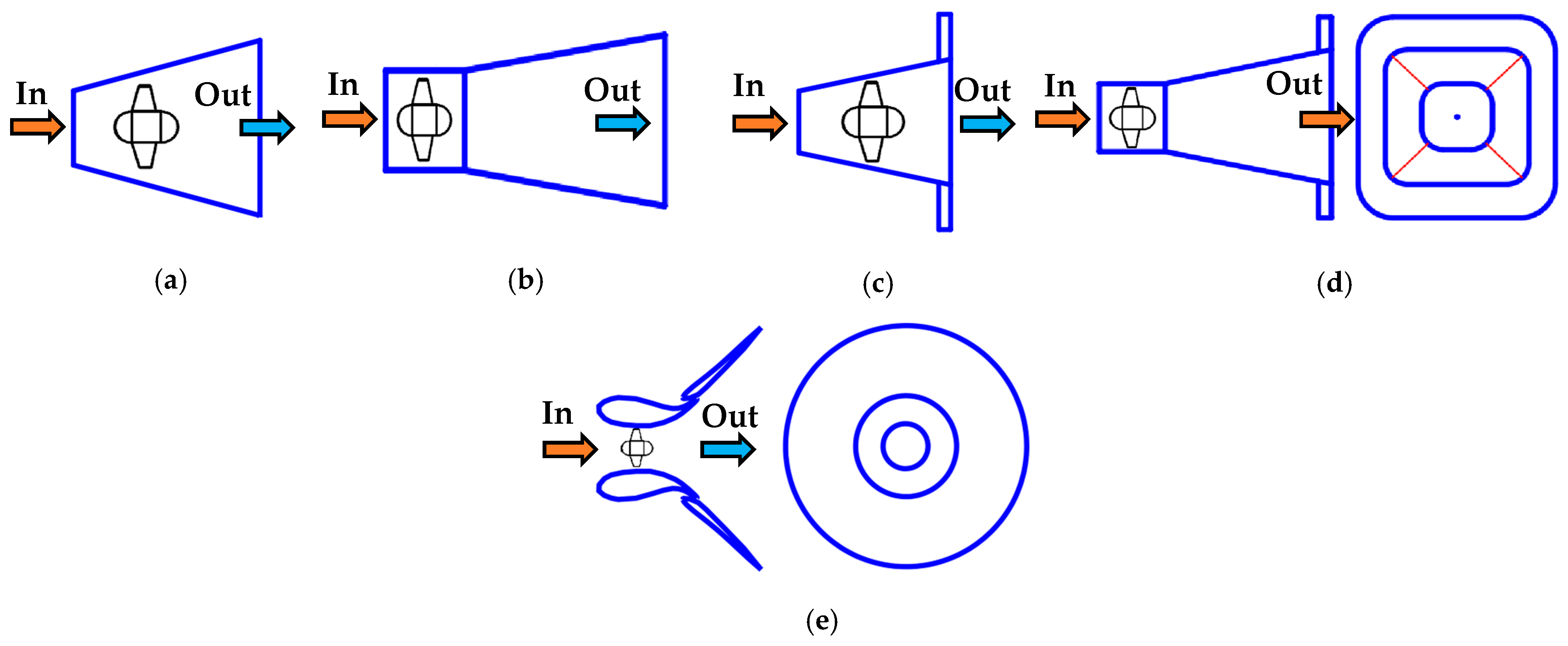
2.3. Summary of Research and Optimization of Hydrokinetic Turbines
| No. | Author(s) | Power Coefficient (Cp) | Method Used | Blade Profile | Water Velocity (m/s) | Rotor Position in the CFD Domain (m) | Dimensions of the Measurement Section (m) | Rotor Main Diameter (m) | Blockage Coeff. | Blade Number | Optimized Parameters |
|---|---|---|---|---|---|---|---|---|---|---|---|
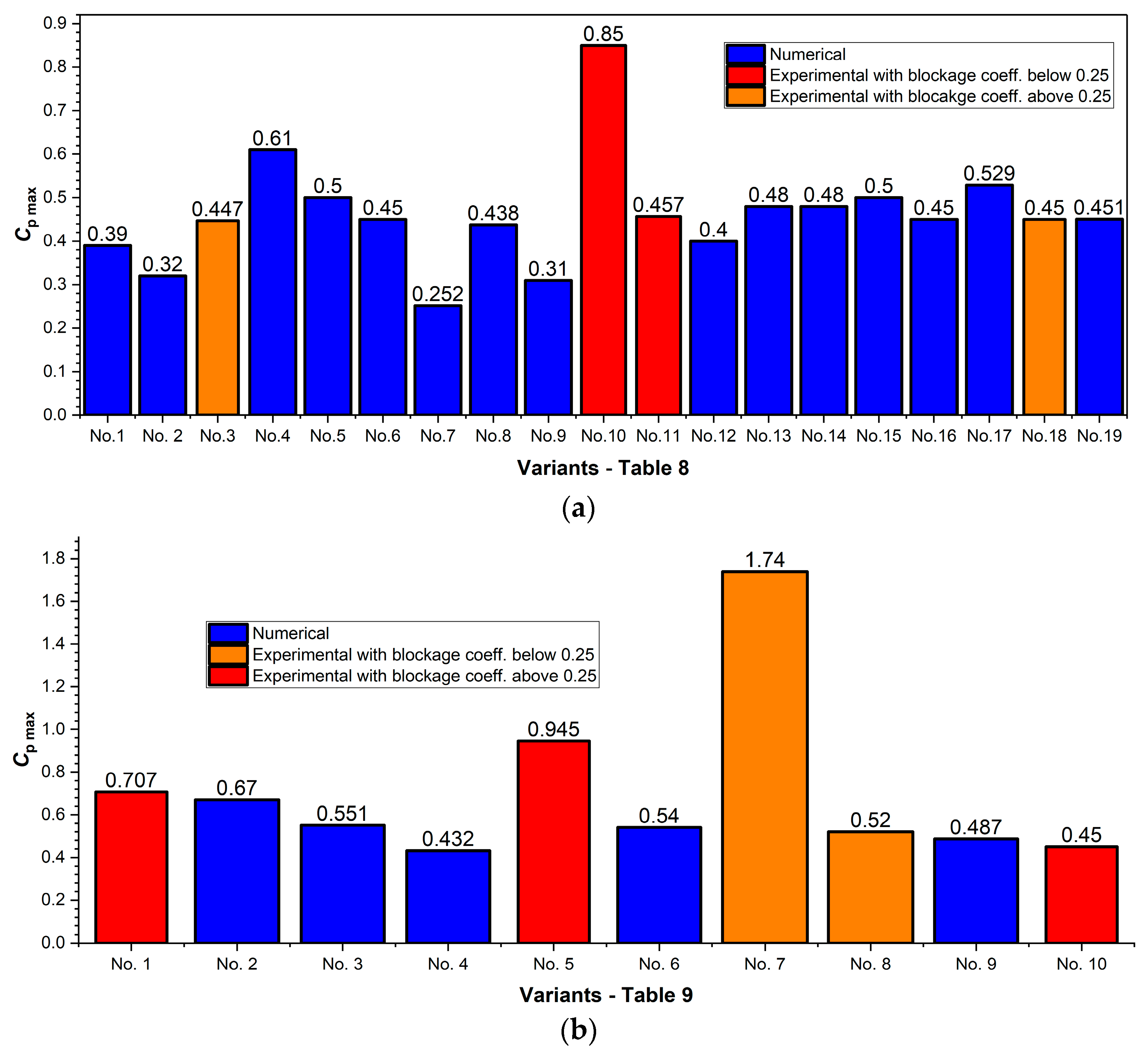
| 1 | Pucci et al. [70] | 0.390 | BEM, CFD comparisons | Wortmann-FX 63-137 | 1.0–1.5 | Inlet dist. 10D1 Outlet dist. 20D1 Wall dist. 4D1 | Not mentioned | 0.900 | - | 3 | Blade pitch angles and chord lengths |
| 2 | Abutunis et al. [57] | 0.320 | BEM, NN (MLP) | Eppler 395 | 0.5–1.0 | Not mentioned | Not mentioned | Not mentioned | - | 3 | |
| 3 | Zhu et al. [71] | 0.447 | BEM, CFD (SST k-ω), NSGA-II, RBF-NN, experiment | Not mentioned | 3.5 | Inlet dist. 5D1 Outlet dist. 10D1 | 0.600 × 0.600 × 1.000 | 5.400 (CFD) 0.240 (exp) | 0.126 | 4 | |
| 4 | Vogel et al. [55] | 0.610 | BEM, CFD (OpenFOAM, SST k-ω) | Not mentioned | 2.2 | Not mentioned | - | 20.000 | - | 3 | Dynamic pitch angle range |
| 5 | Payne et al. [72] | 0.500 | BEM, CFD | NACA 63-8XX series | 0.8 | Not mentioned | - | 1.200 | - | 3 | Blade profile pitch angles, and chord lengths |
| 6 | Nigam et al. [73] | 0.450 | BEM, ANSYS Fluent | E817 (hub), S832 (blade) | 2 | Not mentioned | - | 2.000 | - | 3 | |
| 7 | Wang et al. [56] | 0.252 | CFD (ANSYS Fluent, k-ω SST) | NACA 4412 | 0.8 | Inlet dist. 2D1 Outlet dist. 5D1 | - | 2.000 | - | 3 | |
| 8 | Chica et al. [74] | 0.438 | BEM, CFD (ANSYS CFX, k-ε) | NREL S822 | 1.5 | Not mentioned | - | 1.360 | - | 3 | |
| 9 | Chen et al. [75] | 0.310 | BEM, Wilson’s optimization | Not mentioned | 0.8–2.2 | Not mentioned | - | 3.700 | - | 3 | Blade profile pitch angles, and chord lengths |
| 10 | Patel et al. [54] | 0.850 | Experimental | Not mentioned | 1.9 | Not mentioned | 0.101 × 1.000 | 0.086 | 0.569 | 4 | Tip fillet radius, blade number |
| 11 | Romero et al. [58] | 0.457 | CFD (ANSYS Fluent, k-ω SST), experiment | SG 6043 | 1.5 | Inlet dist. 2.5D1 Outlet dist. 6.25D1 Wall dist. 5D1 | 0.31 × 0.5 × 8.000 | 1.600 (CFD) 0.240 (exp.) | 0.292 | 3 | Skew and wake angles of the blades |
| 12 | Arribas et al. [76] | 0.400 | BEM | NACA 4415, NACA 23015 | 1.5–3.0 | Not mentioned | - | 0.400 | - | 2, 3 and 4 | Blade profile. pitch angles, chord lengths, blade number |
| 13 | Sale et al. [77] | 0.480 | BEM, Genetic Algorithm | NACA 44XX, Risø-A1-XX | 1.0–2.5 | Not mentioned | - | 5.000 | - | 3 | |
| 14 | Chadras et al. [78] | 0.480 | CFD (ANSYS CFX, k-ω SST) | NREL S822 | 1 | Not mentioned | - | 0.800 | - | 3 | Blade swept angles |
| 15 | Li et al. [79] | 0.500 | BEM, ANN, Genetic Algorithm, CFD (Fine/Turbo, Spalart-Allmaras) | NACA 63-418 | 2 | Not mentioned | - | 3.700 | - | 3 | Blade pitch angles and chord lengths |
| 16 | Eriamiatoe et al. [59] | 0.450 | CFD (ANSYS CFX, k-ω SST) | SG6043 | 2 | Not mentioned | - | 2.000 | - | 3 | |
| 17 | Gemaque et al. [80] | 0.529 | Extended BEM | SG6040 | 1 | Not mentioned | - | 0.800 | - | 4 | Blades swept angles |
| 18 | Hanzla et al. [60] | ~0.450 | Experimental | SG6043 | 1 | - | 0.610 × 0.610 × 1.980 | 0.280 | 0.165 | 3 | Blade shape |
| 19 | Wang et al. [81] | 0.451 | BEM, CFD (ANSYS Fluent, URANS, DES) | NACA 63-8XX | 3.4 | Not mentioned | - | 15.200 | - | 3 | Blade number, pitch angles, and chord lengths |
| No. | Authors | Power Coefficient (CP) | Method Used | Blade Profile | Water Velocity (m/s) | Rotor Position in the CFD Domain (m) | Dimensions of the Measurement Section (m) | Rotor Main Diameter (m) | Blockage Coeff. | Blade Num | Optimized Parameters |
|---|---|---|---|---|---|---|---|---|---|---|---|
| 1 | Nishi et al. [63] | 0.707 | CFD (ANSYS CFX 15.0) + Experiment | MEL021, MEL031 | 1.50 (CFD), 1.72 (Exp) | Inlet dist. 10D1 Outlet dist. 15D1 Wall dist. 10D1 | 0.570 × 1.900 | 0.342 | 0.282 | 3 | Blade number, profile, diffuser shape |
| 2 | Tampier et al. [68] | 0.670 | CFD (STAR-CCM+) | Sandia MHKF1 | 2 | Inlet dist. 5D1 Outlet dist. 5D1 Wall dist. 7D1 | - | 2.000 | - | 3 | Rotor position in the diffuser |
| 3 | Song et al. [61] | 0.551 | CFD (ANSYS Fluent) | Not mentioned | 1.5 | Inlet dist. 5D1 Outlet dist. 15D1 Wall dist. 5D1 | - | 2.000 | - | 3 | Diameter of the shaft |
| 4 | Wang et al. [67] | 0.432 | CFD (ANSYS Fluent) | Not mentioned | 2 | Inlet dist. 19.92D1 Outlet dist. 33.2D1 Wall dist. 9.6D1 | - | 0.250 | - | 4 | Diffuser shape |
| 5 | Chihaia et al. [64] | 0.945 | Experimental | Not mentioned | 0.9 | - | 0.300 × 0.300 | 0.200 | 0.349 | 4 | Diffuser shape and rotor position |
| 6 | Parka et al. [62] | 0.540 | CFD (OpenFOAM, DAFoam) | Not mentioned | 1.4 | Inlet dist. 11.4D1 Outlet dist. 19D1 Wall dist. 5.4D1 | - | 0.440 | - | 3 | Diffuser shape |
| 7 | J. Reinecke [66] | 1.740 | CFD (ANSYS Fluent) + Experiment | Not mentioned | 1.5 | - | 4.600 × 9.300 × 90.000 | 0.800 | 0.012 | 3 | Diffuser shape |
| 8 | Góralczyket al. [69] | 0.520 | CFD (Vortex Lattice Method), experiment | Not mentioned | 3.4 | Not mentioned | 0.425 × 0.425 | 0.148 | 0.095 | 5 | Rotor position in the diffuser |
| 9 | Cardona-Mancilla et al. [30] | 0.487 | CFD (ANSYS CFX 18.2) | NREL S822 | 1.5 | Inlet dist. 0.55D1 Outlet dist. 4.875D1 Wall dist. 1.6D1 | - | 0.800 | - | 3 | Diffuser shape |
| 10 | Gish et al. [65] | 0.450 | CFD (SolidWorks FlowSim), experiment | NACA 4412 | 0.61–1.52 | Not mentioned | Not mentioned | 0.265 | - | 3 | Diffuser shape |
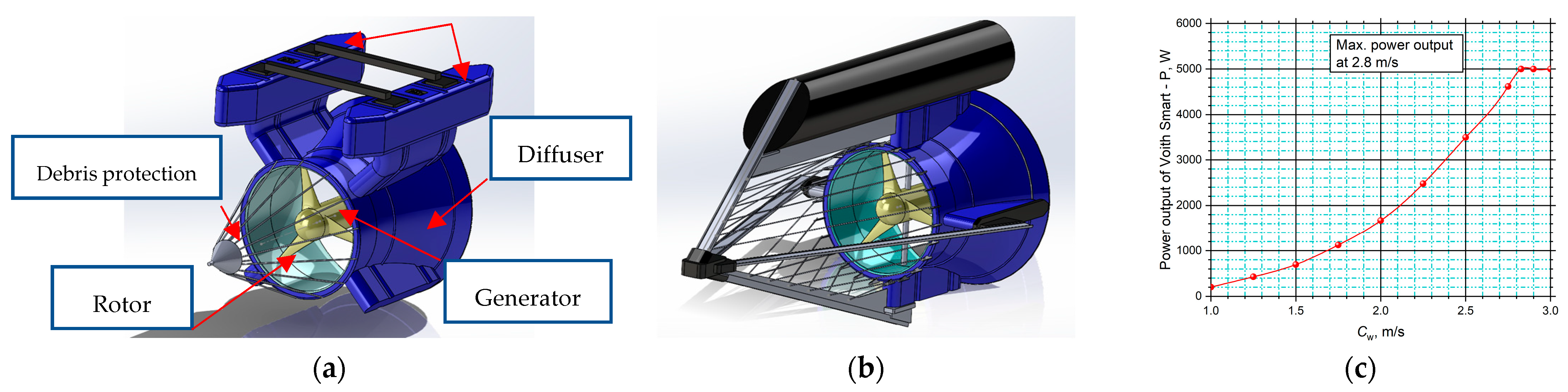
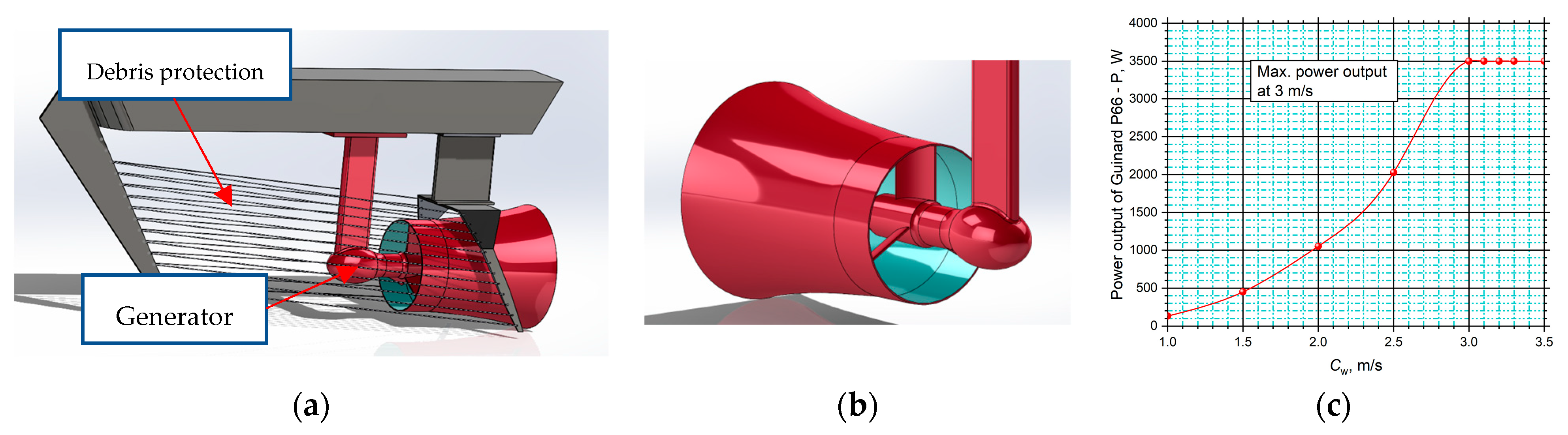
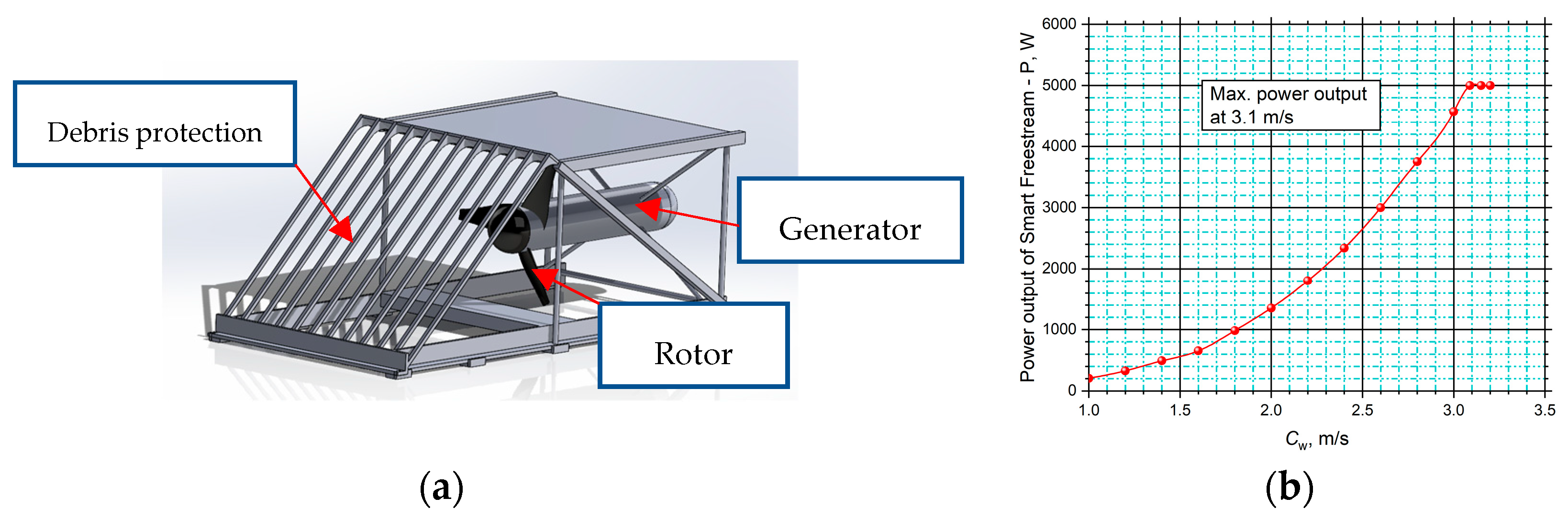
2.4. Specifications of the Commercial Turbines
3. Results
4. Discussion
5. Conclusions
Author Contributions
Funding
Conflicts of Interest
References
- Aristizábal-Tique, V.; Villegas-Quiceno, A.P.; Arbeláez-Pérez, O.F.; Colmenares-Quintero, R.F.; Vélez-Hoyos, F.J. Development of riverine hydrokinetic energy systems in Colombia and other world regions: A review of case studies. DYNA 2021, 88, 256–264. [Google Scholar]
- Zhou, Z.; Benbouzid, M.; Charpentier, J.; Scuiller, F.; Tang, T. Developments in large marine current turbine technologies—A review. Renew. Sustain. Energy Rev. 2017, 71, 852–858. [Google Scholar] [CrossRef]
- Niebuhra, C.M.; Dijka, M.; Nearyb, V.S.; Bhagwanc, J.N. A review of hydrokinetic turbines and enhancement techniques for canal installations: Technology, applicability and potential. Renew. Sustain. Energy Rev. 2019, 113, 109240. [Google Scholar] [CrossRef]
- Yadav, K.P.; Kumar, A.; Jaiswal, S. A critical review of technologies for harnessing the power from flowing water using a hydrokinetic turbine to fulfill the energy need. Energy Rep. 2023, 9, 2102–2117. [Google Scholar] [CrossRef]
- Mancilla, C.C.; Río, J.S.; Arrieta, E.C.; Zuluaga, D.H. Horizontal axis hydrokinetic turbines: A literature review. Tecnol. Cienc. Agua 2018, 9, 180–197. [Google Scholar] [CrossRef]
- Ibrahim, W.I.; Mohamed, M.R.; Ismail, R.M.T.R.; Leung, P.K.; Xing, W.W.; Shah, A.A. Hydrokinetic energy harnessing technologies: A review. Energy Rep. 2021, 7, 2021–2042. [Google Scholar] [CrossRef]
- Iliev, R.; Tsalov, T. Investigation of a cross-flow wind turbine with a hybrid frontal guiding device. Earth Environ. Sci. 2024, 1380, 012001. [Google Scholar] [CrossRef]
- Iliev, R. Investigation of a cross-flow wind turbine with frontal deflector. Earth Environ. Sci. 2024, 1380, 012002. [Google Scholar] [CrossRef]
- Matias, I.J.T.; Danao, L.A.M.; Abuan, B.E. Numerical Investigation on the Effects of Varying the Arclength of a Windshield on the Performance of a Highway Installed Banki Wind Turbine. Fluids 2021, 6, 285. [Google Scholar] [CrossRef]
- Monchwe, T.B. Bernoulli’s principle and the Venturi effect. South Afr. J. Anaesth. Analg. 2023, 29, S42–S44. [Google Scholar]
- Lecanu, P.N.; Mouazé, D.; Bréard, J. Theoretical calculation of wind (Or water) turbine considering kinetic and potential energy to exceed the Betz limit. HoS 2023. [Google Scholar]
- Ledoux, J.; Riffo, S.; Salomon, J. Analysis of the Blade Element Momentum Theory. SIAM J. Appl. Math. 2021, 81, 2596–2621. [Google Scholar] [CrossRef]
- Kravtsoff, F.; Schvallinger, M.; Ottavy, X. A CFD-Based Throughflow Solver Using Cascade Potential Theory for Axial Compressor Flow Modeling. In Turbo Expo: Power for Land, Sea, and Air; American Society of Mechanical Engineers: Houston, TX, USA, 2023. [Google Scholar]
- Anderson, J.D. Computational Fluid Dynamics: The Basics with Applications; McGraw-Hill Education: New York, NY, USA, 2010. [Google Scholar]
- Versteeg, H.K.; Malalasekera, W. An Introduction to Computational Fluid Dynamics: The Finite Volume Method; Pearson Education: London, UK, 2007. [Google Scholar]
- Schlichting, H.; Gersten, K. Boundary-Layer Theory, 8th ed.; Springer: Berlin/Heidelberg, Germany, 2000. [Google Scholar]
- White, F.M. Viscous Fluid Flow, 3rd ed.; McGraw-Hill: New York, NY, USA, 2006. [Google Scholar]
- Lancaster, J.M. Panel Methods in Computational Fluid Dynamics; Elsevier Science: Amsterdam, The Netherlands, 2000. [Google Scholar]
- Theodorsen, T. General Theory of Aerodynamic Instability and the Mechanism of Flutter; Report No. 496; National Advisory Committee for Aeronautics (NACA): Washington, DC, USA, 1935. [Google Scholar]
- Anthoine, L.; Delyon, B. Vortex Lattice Method for the Prediction of the Aerodynamic Forces on a Wing; AIAA: Reston, VA, USA, 1986; Volume 23, pp. 719–724. [Google Scholar]
- Miele, A.; Russo, G. Aerodynamic Shape Optimization: The Vortex Lattice Method; Springer: Berlin/Heidelberg, Germany, 2011. [Google Scholar]
- Todorov, G.; Obretenov, V.; Kamberov, K.; Ivanov, T.; Tsalov, T.; Zlatev, B. Concept and Physical Prototyping of Micro Hydropower System Using Vertical Crossflow Turbine. In Proceedings of the 6th International Symposium on Environment-Friendly Energies and Applications (EFEA), Sofia, Bulgaria, 24–26 March 2021; pp. 1–4. [Google Scholar]
- Todorov, G.; Kamberov, K.; Semkov, M. Improvement of undershot water wheel performance through virtual prototyping. AIP Conf. Proc. 2021, 2333, 110011. [Google Scholar]
- Anthoine, J.; Olivari, D.; Portugaels, D. Wind-tunnel blockage effect on drag coefficient of circular cylinders. Wind. Struct. 2009, 12, 541–551. [Google Scholar] [CrossRef]
- Investigation of Blockage Correction Methods for Full-Scale Wind Tunnel Testing of Trucks. KTH. Available online: https://www.diva-portal.org/smash/get/diva2:893809/FULLTEXT01.pdf (accessed on 13 March 2025).
- López, S. Emerging Trends in Computational Fluid Dynamics. Fluid Mech. 2023, 10, 276. [Google Scholar]
- Vinuesa, R.; Brunton, S. Emerging trends in machine learning for computational fluid dynamics. Comput. Sci. Eng. 2022, 24, 33–41. [Google Scholar] [CrossRef]
- Ji, G.; Dong, J. Computational Fluid Dynamics—Recent Advances, New Perspectives and Applications; IntechOpen: London, UK, 2023. [Google Scholar]
- Badshah, M.; VanZwieten, J.; Badshah, S.; Khalil, S.J. A CFD study of blockage ratio and boundary proximity effects on the performance of a tidal turbine. IET Renew. Power Gener. 2019, 13, 744–749. [Google Scholar] [CrossRef]
- Cardona-Mancilla, C.; Sierra-Del Rio, J.; Hincapié-Zuluaga, D.; Chica, E. A Numerical Simulation of Horizontal Axis Hydrokinetic Turbine with and without Augmented Diffuser. Int. J. Renew. Energy Res. 2018, 8, 1833–1839. [Google Scholar]
- Ren, H.W.; Saat, F.A.Z.M.; Anuar, F.S.; Wahap, M.A.A.; Tokit, E.M.; Tuan, T.B. Computational Fluid Dynamics Study of Wake Recovery for Flow Across Hydrokinetic Turbine at Different Depth of Water. CFD Lett. 2021, 13, 62–76. [Google Scholar] [CrossRef]
- Du, X.; Tan, J.; Yuan, P.; Si, X.; Liu, Y.; Wang, S. Research on the blockage correction of a diffuser-augmented hydrokinetic turbine. Ocean Eng. 2023, 280, 114470. [Google Scholar] [CrossRef]
- Salunkhe, S.; Fajri, O.; Bhushan, S.; Thompson, D.; O’Doherty, D.; O’Doherty, T.; Mason-Jones, A. Validation of Tidal Stream Turbine Wake Predictions and Analysis of Wake Recovery Mechanism. J. Mar. Sci. Eng. 2019, 7, 362. [Google Scholar] [CrossRef]
- Menter, F.R. Zonal Two Equation Kappa-Omega Turbulence Models for Aerodynamic Flows. In AIAA Fluid Dynamics Conference (No. AIAA Paper 93-2906); AIAA: Reston, VA, USA, 1993. [Google Scholar]
- Piomelli, U. Large-eddy simulation: Achievements and challenges. Prog. Aerosp. Sci. 1999, 35, 335–362. [Google Scholar] [CrossRef]
- Lesieur, M.; Metais, O. New trends in large-eddy simulations of turbulence. Annu. Rev. Fluid Mech. 1996, 28, 45–82. [Google Scholar] [CrossRef]
- Spalart, P.R. Comments on the Feasibility of LES for Wings and on the Hybrid RANS/LES Approach. In Proceedings of the First AFOSR International Conference on DNS/LES, Ruston, LA, USA, 4–8 August 1997; pp. 137–147. [Google Scholar]
- Spalart, P.R. Detached-eddy simulation. Annu. Rev. Fluid Mech. 2009, 41, 181–202. [Google Scholar] [CrossRef]
- Kostić, C. Review of the Spalart-Allmaras Turbulence Model and its Modifications to Three-Dimensional Supersonic Configurations. Sci. Tech. Rev. 2015, 65, 43–49. [Google Scholar] [CrossRef]
- Shahed, R.; Mohammadian, A.; Gildeh, A. A comparison of standard k–ε and realizable k–ε turbulence models in curved and confluent channels. Environ. Fluid Mech. 2018, 19, 543–568. [Google Scholar] [CrossRef]
- Wronski, T.; Schönnenbeck, C.; Zouaoui-Mahzoul, N.; Brillard, A. Numerical simulation through Fluent of a cold, confined and swirling airflow in a combustion chamber. Eur. J. Mech.-B/Fluids 2022, 96, 173–187. [Google Scholar] [CrossRef]
- Doran, P. Direct Numerical Simulation. In Bioprocess Engineering Principles, 2nd ed.; Elsevier: Amsterdam, The Netherlands, 2013; pp. 201–254. [Google Scholar]
- ANSYS Fluent User’s Guide. Available online: https://www.ansys.com (accessed on 13 March 2025).
- Ansys CFX Solver Modeling Guide. Available online: https://dl.cfdexperts.net/cfd_resources/Ansys_Documentation/CFX/Ansys_CFX-Solver_Modeling_Guide.pdf (accessed on 13 March 2025).
- OpenFOAM User Guide. Available online: https://www.openfoam.com/documentation/ (accessed on 13 March 2025).
- STAR-CCM+ User Guide. Available online: https://www.plm.automation.siemens.com (accessed on 13 March 2025).
- Autodesk Flow Simulation Technical Documentation. Available online: https://help.autodesk.com (accessed on 13 March 2025).
- Subhra Mukherji, S.; Kolekar, N.; Banerjee, A.; Mishra, R. Numerical investigation and evaluation of optimum hydrodynamic performance of a horizontal axis hydrokinetic turbine. J. Renew. Sustain. Energy 2011, 3, 063105. [Google Scholar] [CrossRef]
- Chihaia, R.; Oprina, G.; Nicolaie, S.; El-Leathey, A.; Babutanu, C.; Nedelcu, A. Assessing the blade chord length influence on the efficiency of a horizontal axis hydrokinetic turbine. In Proceedings of the 2016 International Conference on Hydraulics and Pneumatics—HERVEX, Baile Govora, Romania, 9–11 November 2016. [Google Scholar]
- Antonio, C.P.; Brasil, J.; Mendes, R.C.F.; Wirrig, T.; Noguera, R.; Oliveira, T.F. On the design of propeller hydrokinetic turbines: The effect of the number of blades. J. Braz. Soc. Mech. Sci. Eng. 2019, 41, 253. [Google Scholar]
- Patel, C.; Rathod, V.; Patel, V. Effect of blade count on the performance of shrouded axial flow turbines. Sustain. Energy Technol. Assess. 2024, 65, 103779. [Google Scholar] [CrossRef]
- Q Blade. Available online: https://qblade.org/ (accessed on 13 March 2025).
- X Foil. Available online: https://xfoil.com/?srsltid=AfmBOopY_QIFCmOMJOhpL4XPap72ehTwyoz6MOpYDwsKZCVCaEbh7k1v (accessed on 13 March 2025).
- Patel, C.; Rathod, V.; Patel, V. Experimental Investigations of Hydrokinetic Turbine Providing Fillet at the Leading Edge Corner of the Runner Blades. J. Appl. Fluid Mech. 2022, 16, 865–876. [Google Scholar]
- Vogel, C.R.; Willden, R.H.J.; Houlsby, G.T. Blade element momentum theory for a tidal turbine. Ocean Eng. 2018, 169, 215–226. [Google Scholar] [CrossRef]
- Wang, W.; Yin, R.; Yan, Y. Design and prediction hydrodynamic performance of horizontal axis micro-hydrokinetic river turbine. Renew. Energy 2019, 133, 91–102. [Google Scholar] [CrossRef]
- Abutunis, A.; Hussein, R.; Chandrashekhara, K. A neural network approach to enhance blade element momentum theory performance for horizontal axis hydrokinetic turbine application. Renew. Energy 2019, 136, 1281–1293. [Google Scholar] [CrossRef]
- Romero-Menco, F.; Betancour, J.; Velásquez, L.; Rubio-Clemente, A.; Chica, E. Horizontal-axis propeller hydrokinetic turbine optimization by using the response surface methodology: Performance effect of rake and skew angles. Ain Shams Eng. J. 2024, 15, 102596. [Google Scholar] [CrossRef]
- Eriamiatoe, S.; Udo, U. Optimization of Horizontal Axis Hydrokinetic Turbine Performances using Computational Fluid Dynamics (CFD). IOSR J. Mech. Civ. Eng. 2020, 17, 1–6. [Google Scholar]
- Hanzla, M.; Banerjee, A. Spectral behavior of a horizontal axis tidal turbine in elevated levels of homogeneous turbulence. Appl. Energy 2024, 380, 124842. [Google Scholar] [CrossRef]
- Song, K.; Yang, B. A Comparative Study on the Hydrodynamic-Energy Loss Characteristics between a Ducted Turbine and a Shaftless Ducted Turbine. J. Mar. Sci. Eng. J. Mar. Sci. Eng. 2021, 9, 930. [Google Scholar] [CrossRef]
- Parka, J.; Knighta, B.G.; Liao, Y.; Manganob, M.; Pacinib, B.; Makia, K.J.; Martinsb, A.J.R.R.; Suna, J.; Pana, Y. CFD-based Design Optimization of Ducted Hydrokinetic Turbines. Sci. Rep. 2023, 13, 17968. [Google Scholar] [CrossRef]
- Nishi, Y.; Inagaki, T.; Li, Y.; Hirama, S.; Kikuchi, N. Study on Performance Improvement of an Axial Flow Hydraulic Turbine with a Collection Device. Int. J. Fluid Mach. Syst. 2016, 9, 47–55. [Google Scholar] [CrossRef]
- Chihaia, R.; El-Leathey, L.; Cîrciumaru, G.; Tănase, N. Increasing the energy conversion efficiency for shrouded hydrokinetic turbines using experimental analysis on a scale model. In E3S Web of Conferences; EDP Sciences: Les Ulis, France, 2019. [Google Scholar]
- Gish, L.A.; Hawbaker, G. Experimental and Numerical Study on Performance of Shrouded Hydrokinetic Turbines. In Proceedings of the OCEANS 2016 MTS/IEEE Monterey, Monterey, CA, USA, 19–23 September 2016. [Google Scholar]
- Reinecke, J. Effect of a Diffuser on the Power Production of Ocean Current Turbines. Ph.D. Thesis, University of Stellenbosch, Stellenbosch, South Africa, 2011. [Google Scholar]
- Wang, B.; Yu, Y.; Niu, X. A parametric analysis of the performance of a horizontal axis tidal current turbine for improving flow-converging effect. Ocean Eng. 2024, 291, 116481. [Google Scholar] [CrossRef]
- Tampier, G.; Troncoso, C.; Zilic, F. Numerical analysis of a diffuser-augmented hydrokinetic turbine. Ocean Eng. 2017, 145, 138–147. [Google Scholar] [CrossRef]
- Góralczyk, A.; Adamkowski, A. Model of a ducted axial-flow hydrokinetic turbine—Results of experimental and numerical examination. Pol. Marit. Res. 2018, 25, 113–122. [Google Scholar] [CrossRef]
- Pucci, M.; Garbo, C.D.; Bellafiore, D.; Zanforlin, S.; Umgiesser, G. A BEM-Based Model of a Horizontal Axis Tidal Turbine in the 3D Shallow Water Code SHYFEM. J. Mar. Sci. Eng. 2022, 10, 1864. [Google Scholar] [CrossRef]
- Zhu, F.; Ding, L.; Huang, B.; Bao, M.; Liu, J. Blade design and optimization of a horizontal axis tidal turbine. Ocean Eng. 2020, 195, 106652. [Google Scholar] [CrossRef]
- Payne, G.S.; Stallard, T.; Martinez, R. Design and manufacture of a bed supported tidal turbine model for blade and shaft load measurement in turbulent flow and waves. Renew. Energy 2017, 107, 312–326. [Google Scholar] [CrossRef]
- Nigama, S.; Bansal, S.; Nema, T.; Sharma, V.; Singh, R.K. Design and Pitch Angle Optimisation of Horizontal Axis Hydrokinetic Turbine with Constant Tip Speed Ratio. MATEC Web Conf. 2016, 95, 06004. [Google Scholar] [CrossRef]
- Chica, E.; Perez, F.; Rubio-Clemente, A.; Agudelo, S. Design of a hydrokinetic turbine. Energy Sustain. 2015, 195, 137–148. [Google Scholar]
- Chen, J.; Wang, X.; Li, H.; Jiang, C.; Bao, L. Design of the Blade under Low Flow Velocity for Horizontal Axis Tidal Current Turbine. J. Mar. Sci. Eng. 2020, 8, 989. [Google Scholar] [CrossRef]
- Arribas, F.P. Hydrodynamic design of rotor blades of marine current turbines. In IOP Conference Series: Earth and Environmental Science; IOP Publishing: Bristol, UK, 2019. [Google Scholar]
- Sale, D. Hydrodynamic Optimization Method and Design Code for Stall-Regulated Hydrokinetic Turbine Rotors; No. NREL/CP-500-45021; National Renewable Energy Lab. (NREL): Golden, CO, USA, 2009. [Google Scholar]
- Chandras, P.; Sharma, L.; Chatterjee, D. Numerical prediction of the performance of axialflow hydrokinetic turbine. In Proceedings of the MARINE: V International Conference on Computational Methods in Marine Engineering, Hamburg, Germany, 29–31 June 2013. [Google Scholar]
- Li, Z.; Li, G.; Du, L.; Guo, H.; Yuan, W. Optimal design of horizontal axis tidal current turbine blade. Ocean Eng. 2023, 271, 113666. [Google Scholar] [CrossRef]
- Gemaque, M.L.A.; Vaz, J.R.P.; Saavedra, O.R. Optimization of Hydrokinetic Swept Blades. Sustainability 2022, 14, 13968. [Google Scholar] [CrossRef]
- Wang, P.; Wang, L.; Zhang, Q.; Zhu, F.; Huang, B. A model for predicting the unsteady hydrodynamic characteristics on the blades of a horizontal axis tidal turbine. Appl. Math. Model. 2024, 127, 506–528. [Google Scholar] [CrossRef]
- Saupi, A.F.M.; Mailah, N.F.; Radzi, M.A.M.; Mohamad, K.B.; Ahmad, S.Z.; Soh, A.C. An Illustrated Guide to Estimation of Water Velocity in Unregulated River for Hydrokinetic Performance Analysis Studies in East Malaysia. Water 2018, 10, 1330. [Google Scholar] [CrossRef]
- Kos, Ž. Ðurin, B.; Dogan, D.; Kranj. Hydro-Energy Suitability of Rivers Regarding Their Hydrological and Hydrogeological Characteristics. Water 2021, 13, 1777. [Google Scholar] [CrossRef]
- Oladeji, A.S.; Akorede, M.F.; Mohammed, A.A.; Adeogun, A.G.; Salami, A.W. Investigation of small hydropower potential of river oshininkwara. Arid. Zone J. Eng. Technol. Environ. 2020, 16, 321–336. [Google Scholar]
- Kayastha, R.; Kayastha, R.B.; Shrestha, K.L.; Gurung, S. Hydropower potential of the Marsyangdi River and Bheri River basins of Nepal and their sensitivity to climate variables. Proc. IAHS 2024, 387, 53–58. [Google Scholar] [CrossRef]
- Smart Hydro Power. Available online: https://www.smart-hydro.de (accessed on 13 March 2025).
- Guinard Energies. Available online: https://www.guinard-energies.bzh/en/our-products/p66-hydrokinetic-turbine-3-5-kw/ (accessed on 13 March 2025).
- Smart Hydro Power. Available online: https://smart-hydro.de/wp-content/uploads/2015/12/Datasheet_SMART_Freestream.pdf (accessed on 13 March 2025).


| Method | Description | Accuracy | Application |
|---|---|---|---|
| Computational Fluid Dynamics (CFD) [14,15,16] | Solves the Navier–Stokes equations for detailed flow prediction, including separation. | Very high (for fully viscous flow) | Predicting separation for real-world complex conditions, including turbulence and separation. |
| Boundary layer theory [17,18] | Applies to inviscid and viscous flows to estimate the separation point based on pressure gradients. | Moderate to high (for laminar flow) | Small angles of attack, simple analysis, or where flow separation is weak. |
| Panel method (vortex panels) [19,20] | Inviscid flow method, not suitable for predicting separation directly. | Low to moderate | Predicts potential flow in the absence of viscosity; needs hybrid methods for separation. |
| Vortex lattice method (VLM) [21] | Similar to panel methods, used for inviscid analysis and lift prediction but doesn’t predict separation. | Moderate to low | Lift predictions, primarily for inviscid flow. |
| Number of Blades (Z) | Max. Powe Coeff (Cp) | Tip Speed Ratio (TSR) at Max Cp | Solidity (σ) |
|---|---|---|---|
| 2 | 0.38 | TSR = 3.5 | 0.064 |
| 3 | 0.41 | TSR = 3.0 | 0.095 |
| 4 | 0.39 | TSR = 3.0 | 0.127 |
| Blade Design | Max Cp | Optimal TSR | Power Output Improvement |
|---|---|---|---|
| Base Variant (Constant Chord) | 0.40 | 1.57–2.0 | Baseline |
| Optimized (Variable Chord) | 0.45 | 1.57–2.62 | +7–8% higher power |
| Number of Blades | Maximum Cp | Tip Speed Ratio (TSR) at Max Cp |
|---|---|---|
| 2-Blade Runner | 0.30–0.36 | 1.6–2.0 |
| 3-Blade Runner | 0.39–0.41 | 1.5–1.8 |
| 4-Blade Runner | 0.39–0.40 | 1.4–1.6 |
| Blade Count (N) | Max CP | TSR at Max CP |
|---|---|---|
| 2 Blades | 0.25 | 1.72 |
| 3 Blades | 0.35 | 1.70 |
| 4 Blades | 0.45 | 1.67 |
| 5 Blades | 0.36 | 2.18 |
| 6 Blades | 0.28 | 1.32 |
| 7 Blades | Did not rotate | 0 |
| No. | River, Theoretical Velocity Range (m/s) | Bare Turbines—Table 8 | Shrouded Turbines—Table 9 |
|---|---|---|---|
| 1 | Batang Balleh (1.80–2.50) [82] | 4, 6, 9, 12, 13, 15, 16 | 1, 2, 4 |
| 2 | Bednja (0.50–1.10) [83] | 1, 5, 7, 9, 14, 17, 18 | 5, 10 |
| 3 | Gornja Dobra (0.65–1.50) [83] | 1, 2, 5, 7, 9, 12, 13, 14, 17, 18 | 1, 3, 5, 6, 7, 9, 10 |
| 4 | Mirna (0.40–1.10) [83] | 1, 2, 5, 9, 14, 17, 18 | 5, 10 |
| 5 | Oshin (0.18–2.08) [84] | 1, 2, 5, 6, 7, 8, 9, 10, 11, 12, 13, 14, 15, 16, 17, 18 | 1, 2, 3, 5, 6, 7, 9, 10 |
| 6 | Marsyangdi (1.00–2.10) [85] | 1, 2, 5, 6, 7, 8, 9, 10, 11, 12, 13, 14, 15, 16, 17, 18 | 1, 2, 3, 4, 6, 7, 9 10 |
| 7 | Bheri (1.30–2.40) [85] | 1, 4, 6, 8, 9, 10, 11, 12, 13, 14, 15, 16, 17, 18 | 1, 2, 3, 4, 6, 7, 9, 10 |
| Selected Bare Turbines | Voith | Genuard P66 | Smart Freestream | |||||
|---|---|---|---|---|---|---|---|---|
| No. | Author(s) | Power Coefficient (Cp) | Water Velocity (m/s) | Rotor Main Diameter (m) | Blade Number | Power Coefficient (Cp) | ||
| 1 | Pucci et al. [70] | 0.390 | 1.5 | 0.900 | 3 | 0.514 | 0.867 | 0.450 |
| 2 | Abutunis et al. [57] | 0.320 | 1.0 | Not mentioned | 3 | 0.383 | 0.879 | 0.383 |
| 3 | Zhu et al. [71] | 0.447 | 3.5 | 0.240 | 4 | 0.635 | 0.471 | 0.348 |
| 4 | Vogel et al. [55] | 0.610 | 2.2 | 20.000 | 3 | 0.557 | 0.737 | 0.422 |
| 5 | Payne et al. [72] | 0.500 | 0.8 | 1.200 | 3 | 0.320 | 0.857 | 0.323 |
| 6 | Nigam et al. [73] | 0.450 | 2 | 2.000 | 3 | 0.542 | 0.732 | 0.415 |
| 7 | Wang et al. [56] | 0.252 | 0.8 | 2.000 | 3 | 0.320 | 0.857 | 0.323 |
| 8 | Chica et al. [74] | 0.438 | 1.5 | 1.360 | 3 | 0.514 | 0.867 | 0.450 |
| 9 | Chen et al. [75] | 0.310 | 2.2 | 3.700 | 3 | 0.557 | 0.737 | 0.422 |
| 10 | Patel et al. [54] | 0.850 | 1.9 | 0.086 | 4 | 0.524 | 0.744 | 0.424 |
| 11 | Romero et al. [58] | 0.457 | 1.5 | 0.240 | 3 | 0.514 | 0.867 | 0.450 |
| 12 | Arribas et al. [76] | 0.400 | 3.0 | 0.400 | 4 | 0.472 | 0.759 | 0.425 |
| 13 | Sale et al. [77] | 0.480 | 2.5 | 5.000 | 3 | 0.571 | 0.750 | 0.430 |
| 14 | Chadras et al. [78] | 0.480 | 1.0 | 0.800 | 3 | 0.383 | 0.879 | 0.383 |
| 15 | Li et al. [79] | 0.500 | 2.0 | 3.700 | 3 | 0.542 | 0.732 | 0.415 |
| 16 | Eriamiatoe et al. [59] | 0.450 | 2.0 | 2.000 | 3 | 0.542 | 0.732 | 0.415 |
| 17 | Gemaque et al. [80] | 0.529 | 1.0 | 0.800 | 4 | 0.383 | 0.879 | 0.383 |
| 18 | Hanzla et al. [60] | 0.450 | 1.0 | 0.280 | 3 | 0.383 | 0.879 | 0.383 |
| 19 | Wang et al. [81] | 0.451 | 3.4 | 15.200 | 3 | 0.601 | 0.554 | 0.353 |
| Selected Shrouded Turbines | Voith | Genuard P66 | Smart Freestream | |||||
|---|---|---|---|---|---|---|---|---|
| No. | Authors | Power Coefficient (CP) | Water Velocity (m/s) | Rotor Main Diameter (m) | Blade Number | Power Coefficient (CP) | ||
| 1 | Nishi et al. [63] | 0.707 | 1.72 | 0.342 | 3 | 0.500 | 0.802 | 0.438 |
| 2 | Tampier et al. [68] | 0.607 | 2 | 2.000 | 3 | 0.542 | 0.732 | 0.415 |
| 3 | Song et al. [61] | 0.551 | 1.5 | 2.000 | 3 | 0.514 | 0.867 | 0.450 |
| 4 | Wang et al. [67] | 0.432 | 2 | 0.250 | 4 | 0.542 | 0.732 | 0.415 |
| 5 | Chihaia et al. [64] | 0.732 | 0.9 | 0.200 | 4 | 0.324 | 0.869 | 0.348 |
| 6 | Parka et al. [62] | 0.540 | 1.4 | 0.440 | 3 | 0.519 | 0.879 | 0.465 |
| 7 | J. Reinecke [66] | 1.740 | 1.5 | 0.800 | 3 | 0.514 | 0.867 | 0.450 |
| 8 | Góralczyk et al. [69] | 0.520 | 3.4 | 0.148 | 5 | 0.601 | 0.554 | 0.353 |
| 9 | Cardona-Mancilla et al. [30] | 0.487 | 1.5 | 0.800 | 3 | 0.514 | 0.867 | 0.450 |
| 10 | Gish et al. [65] | 0.450 | 1.52 | 0.265 | 3 | 0.513 | 0.865 | 0.447 |
Disclaimer/Publisher’s Note: The statements, opinions and data contained in all publications are solely those of the individual author(s) and contributor(s) and not of MDPI and/or the editor(s). MDPI and/or the editor(s) disclaim responsibility for any injury to people or property resulting from any ideas, methods, instructions or products referred to in the content. |
© 2025 by the authors. Licensee MDPI, Basel, Switzerland. This article is an open access article distributed under the terms and conditions of the Creative Commons Attribution (CC BY) license (https://creativecommons.org/licenses/by/4.0/).
Share and Cite
Iliev, R.; Todorov, G.; Kamberov, K.; Zlatev, B. Evaluation of the Performance of Optimized Horizontal-Axis Hydrokinetic Turbines. Water 2025, 17, 1532. https://doi.org/10.3390/w17101532
Iliev R, Todorov G, Kamberov K, Zlatev B. Evaluation of the Performance of Optimized Horizontal-Axis Hydrokinetic Turbines. Water. 2025; 17(10):1532. https://doi.org/10.3390/w17101532
Chicago/Turabian StyleIliev, Rossen, Georgi Todorov, Konstantin Kamberov, and Blagovest Zlatev. 2025. "Evaluation of the Performance of Optimized Horizontal-Axis Hydrokinetic Turbines" Water 17, no. 10: 1532. https://doi.org/10.3390/w17101532
APA StyleIliev, R., Todorov, G., Kamberov, K., & Zlatev, B. (2025). Evaluation of the Performance of Optimized Horizontal-Axis Hydrokinetic Turbines. Water, 17(10), 1532. https://doi.org/10.3390/w17101532