Abstract
This paper presents a comprehensive approach to forecasting hydro–meteorological changes in a marine area, i.e., in large bodies of water, from open water to coastal zones. First, hydro–meteorological factors, their interactions, and their implications for marine ecosystems are described. In addition, an analysis is outlined specifically for the Baltic Sea area. Next, the procedure for forecasting expected changes in major hydro–meteorological parameters in the sea is presented and a series of steps is accurately described. An extensive prognosis is provided for the southern Baltic Sea region using historical data obtained from the Polish National Institute of Water Management and Meteorology. The procedure is applied for seven measurement points which were assigned to four sub-areas for examining trends in wind regimes and wave height patterns using the authors’ own written software and statistical methods for data analysis. The model was validated within the southern Baltic Sea region. This paper also highlights the significance of forecasting for human beings, the environment, and critical infrastructure by proposing adaptive strategies and integrated coastal zone management in mitigating risks and enhancing resilience. Finally, future directions for research are proposed.
1. Introduction
Since ancient times, humans have been keenly observing weather patterns, particularly those that are adverse. Hydro–meteorological information plays a critical role in ensuring navigation safety at sea and in inland waterways [1]. The monitoring and prediction of meteorological and hydrological elements are essential for minimizing financial losses within port companies and the maritime transportation sector [2]. Atmospheric circulation, pressure levels, wind characteristics, temperature variations, humidity levels, evaporation rates, precipitation patterns, snow accumulation, storm occurrences, insolation levels, and cloud formations are all part of meteorological conditions [3]. They refer to the various phenomena that influence weather patterns and climate and can have significant impacts on communities and ecosystems. Among the hydrological and hydrodynamic factors considered are sea water levels, currents, water exchange, waves, and icing [1,4]. Recently, there has been a noticeable rise in the intensity and occurrence frequency of hazardous hydrological events [5].
The interactions between meteorological (weather patterns), hydrological (water cycles), and hydrodynamic (movement of water bodies) conditions are very complex and have significant implications for marine ecosystems [6]. Together, they offer critical insights into the functioning of Earth’s climate system, influencing everything from global weather patterns to local marine ecosystems.
Variations in atmospheric pressure can lead to changes in sea level. Areas of low pressure can cause sea levels to rise locally, while areas of high pressure can cause sea levels to fall (inverted barometric effect, except for the regions close to the equator) [7]. These changes can influence tidal patterns, fishery yields, and the accessibility of ports and harbors.
Wind speed and direction, especially along coastlines, can affect upwelling processes, bringing nutrient-rich waters to the surface and supporting high levels of primary biological productivity [8,9]. Downwelling occurs when winds push surface water towards the coast, forcing it downward and potentially transporting oxygen to deeper areas. On the other hand, wind-driven currents and waves can traverse vast distances, not only redistributing heat across the globe and influencing climate patterns, but also transporting nutrients, organisms, and pollutants in the water column [10,11].
Extreme events like storms or hurricanes can lead to storm surges, where strong winds push water toward the shore, temporarily raising sea levels above normal high tides. This can cause significant coastal flooding and dramatically alter hydrodynamic conditions [12]. Advanced understanding aids in predicting these hazards, minimizing risks for aquaculture, fishing, maritime transport, and recreational marine activities. Furthermore, the combination of strong winds and elevated ocean water levels that trigger storm surges not only increases sea levels but also contributes to the reduction in soil moisture in coastal areas [12]. This can have cascading effects on local ecosystems, agriculture, and freshwater resources.
Meteorological conditions, particularly temperature and wind, influence the formation and melting of sea ice [13]. Ice formation affects the salinity and density of surrounding waters, playing a critical role in circulation. Wind can break up ice floes, affecting the albedo (reflectivity) of the surface and local weather patterns. Changes in atmospheric temperature influence sea temperatures and ice melt, which, in turn, affect sea levels. Understanding these dynamics is crucial for predicting future climate scenarios and their impact on marine biodiversity and coastal communities.
Meteorological conditions affect evaporation rates from the sea surface and precipitation patterns, which, in turn, influence salinity and surface water density [14]. These factors are crucial for the formation of water masses and the driving of thermohaline circulation, a global conveyor belt of ocean currents that plays a key role in regulating Earth’s climate.
The contextualization of hydro–meteorological conditions within the broader fields of climate science and maritime studies is essential for a comprehensive understanding of our planet’s climate system and its impacts on marine environments. The climate resilience and adaptation strategies for coastal communities vulnerable to extreme weather events and changing conditions may include the implementation of sustainable coastal defense measures, ecosystem restoration projects, and the development of early warning systems for natural disasters [15]. Effective coastal management practices must account for the risks of erosion, flooding, and damage to properties and critical facilities, incorporating climate data and predictive models to safeguard communities and ecosystems. Also, research indicates that meteorological factors can affect the quality of water in various water bodies and impact the water supply system [16]. Moreover, coastal and marine tourism, including beaches, diving, and wildlife viewing, can be significantly impacted by changes in weather patterns, sea conditions, and the health of marine ecosystems. The deployment of advanced observational technologies, like satellite remote sensing and autonomous underwater vehicles, to gather data on sea conditions and climate change impacts may improve our understanding of how hydro–meteorological conditions interact.
In the face of climate change, extreme weather hazards may be increasing. It is anticipated that future climatic changes will be accompanied by growing fluctuations in time as well as a variation in mean values, such as temperature or wind speed. In order to predict and mitigate their current and future impact on critical infrastructure safety and the functioning of ecosystems, we should be able to determine the parameters of the model that embraces hydro–meteorological changes. Particularly, when applying stochastic models to forecast the dynamics of the process of hydro-meteorological changes, it is essential to accurately determine its probability of staying at its current state, analyze transitions between various states, and identify the relevant distribution functions effectively [17,18]. The ways to determine unknown parameters of the hydro–meteorological change process model and to evaluate the process’ characteristics are presented in this paper and carried out for the southern Baltic Sea area. The methodology proposed has been validated within the southern Baltic Sea region, demonstrating high accuracy and reliability in forecasting hydro–meteorological conditions. Through data analysis, model calibration, and local institute engagement, the authors have confirmed the effectiveness of the model.
Forecasting hydro–meteorological changes in marine areas is critical for navigation safety, coastal zone management, and understanding climate change impacts. Previous studies have emphasized the need for accurate and comprehensive forecasting models since many existing machine-learning models do not consider related variables in their inputs [19] or are computing arithmetic operations with less numerical precision [20]. The stochastic-based procedure proposed in this paper integrates associated factors as part of the input data with the highest possible numerical precision available, creating a more comprehensive multivariate model. This paper also goes a step further by detailing the process of integrating meteorological, hydrological, and hydrodynamic conditions. The employed semi-Markov approach considered, e.g., in Refs. [21,22] to forecast the changes of hydro–meteorological conditions, allows for more accurate prediction of probabilities and mean values staying in different states than the Markov approach offers, as the transition times between states do not have to be assumed to be exponential. The approach used in this paper, involving the use of authors’ own customized software combined with statistical methods for analyzing hydro–meteorological condition changes, represents a significant contribution to the field, offering a potentially replicable model for other regions.
2. Baltic Sea Hydro–Meteorological Conditions, Their Interactions, and Patterns in Other Environments
The Baltic Sea, located in Northern Europe, is a semi-enclosed sea with a limited exchange of water with the North Sea through the Danish Straits. The Baltic is surrounded by countries with varied climates. Its unique characteristics result in distinct hydro–meteorological patterns influenced by geographical location and regional atmospheric conditions, land–sea interactions, and anthropogenic factors [1,23]. It is notably impacted by North Atlantic oscillation in winter, which shows a cascading effect on other meteorological parameters. The southwestern part of the sea experiences fairly mild conditions, although periods of unsettled weather with strong winds and rough seas can occur [24].
2.1. Hydro–Meteorological Conditions in the Baltic Sea
The hydro–meteorological conditions of the Baltic Sea are defined by the unique characteristics of this basin. Southwest winds with high speeds occur frequently in the Baltic Sea region, typically in the Baltic Proper [25]. East of Rugen Island and south of Bornholm Island are the places with the strongest winds and highest storm frequency. Compared to most other coastal areas, this area has more than twice the rate of severe winds and more than three times the frequency of storms. The wind patterns in this windy area are similar to those in Skagerrak and Kattegat [26]. Along the Estonian coastline in the Danish Straits and at the end of the northern gulfs and bays, the mean wind speeds are generally lower. Strong winds occur in the Baltic Sea more frequently than in the North Sea but relative storm frequencies are lower overall.
Prevailing winds come from the west, leading to the usual transport of air pollutants from west to east. Additionally, the surface water of the Baltic Sea circulates constantly and anticlockwise, allowing marine pollutants from southern regions to travel along the eastern and northern coastal areas before returning southward. Winds blowing at speeds of 17 m/s or higher can cause significant disruptions to ferry and other ship traffic, damage electricity cables and other structures, and generate large waves along the coast, resulting in localized flooding [27,28].
In the Baltic Proper, wind speeds are usually 5.5 m/s–10 m/s throughout the year [23]. During winter months, especially November, the highest (mostly from the southwest) wind speeds are noticeable, while May exhibits rather weak wind speeds with northerly and easterly directions. However, southerly winds dominate in late winter for many sea regions and are fairly unstable. Easterly winds prevail near the Swedish coast.
The yearly trend of severe winds and storms for the “Baltic storm centre” south of Bornholm is shown in Figure 1.
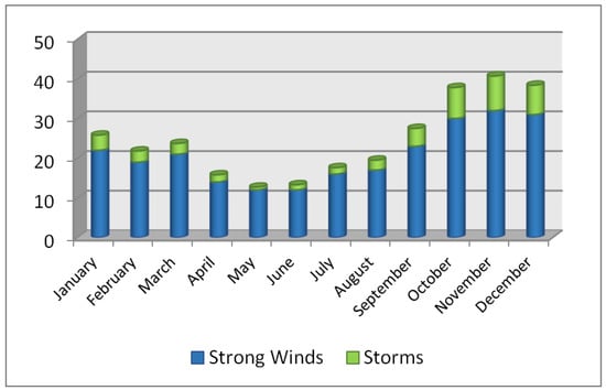
Figure 1.
Frequency of strong winds and storms south of Bornholm [29].
Between August and October, there is a significant rise in the frequency of strong winds and storms, while there is a noticeable decline in the early winter, followed by a decrease between March and April. In March, the center of strong wind and storm activity shifts to the western Baltic Sea, whereas during August and September, it extends from the area east of Rugen to the central Baltic Sea [29,30].
The Baltic Sea is characterized as stormy, with an average of about three storms per year. Waves tend to be short and steep, with the highest waves reaching approximately 10 m in the late autumn or in the winter, but, typically, they are about half that value. In many regions of the Baltic Sea, especially restricted or semi-restricted, low waves prevail throughout the year [31], yet some central open areas can encounter moderate waves more frequently, with exceptional instances of waves reaching heights of up to 8 m [23].
In most regions, waves predominantly approach from southwesterly directions. However, during the summer, there is a shift towards more westerly or even northwesterly directions. In the late spring, both wind and wave directions are highly unstable, leading to variability even among adjacent areas.
Water levels in the Baltic Sea are primarily influenced by wind through two main mechanisms: the creation of a slope that results in significant deviations and the induction of fluctuations from water transport entering or exiting the basin. However, the magnitude typically remains below half a meter. Throughout the basin, extreme sea levels usually take place predominantly during the winter.
Over the past few decades, annual precipitation varied considerably across the Baltic Sea region, with the highest amounts observed in the southwest. Precipitation levels sharply decreased but, moving eastward along the southern coast, they generally increased. Areas over the open sea, as indicated by data from the islands, generally received lower precipitation. Notably, stations on the western coast of the central Baltic Sea received significantly less rainfall compared to those on the eastern coast, possibly due to the leeward effect of the Scandinavian Mountains [24].
During normal and mild winters, the ice cover spans 15–50% of the sea area in the northeastern part of the sea but can extend to the entire basin during infrequent severe winters. Maximum ice coverage typically occurs in February or March, and sea ice usually persists in the Bothnian Sea until mid-May [32].
In terms of visibility, visibility less than 1 km is considered foggy, regardless of the cause. Fog, while infrequent over open waters, is most prevalent in narrow channels and inlets during winter and spring. Visibility is typically good during the year, while fog occurs less frequently in the summer and more commonly in spring as air temperatures rise while the water remains cold [33].
The climate differs between the north and south due to the long extension of the basin [34]. The average annual highest water temperatures in the Baltic Sea generally occur in the southern waters, while the coldest are in the north. Generally, the coasts and continents are colder than the sea, which is typical for northern regions. The water temperature usually is between −0.5 °C and +20.0 °C. Additionally, the bottom water temperature remains constant regardless of the season (2 °C–4 °C), while the temperature of the wind-mixed surface water varies with the season.
The mean annual air temperature is around 0 °C in the north and 8 °C–12 °C in the south. Surface air temperatures have increased since the 1870s, leading to changes in the seasons: the warm season has lengthened, while the cold season has shortened [35].
2.2. Baltic Sea Regional Specifity and Potential Variations in Hydro–Meteorological Patterns in Other Marine Environments
Marine environments are influenced by a multitude of factors, including geographical location, currents, atmospheric conditions, and local topography, all of which contribute to the unique hydro–meteorological patterns observed in different areas. Each marine environment, therefore, exhibits its own set of characteristics, driven by different climatic and oceanographic processes. When contrasting the Baltic Sea with other seas regarding the impact of hydro–meteorological conditions, these several distinct factors highlight its unique position and the challenges it faces.
Seasonal and climatic variability in the Baltic Sea is marked by extreme changes, including significant ice cover in winter, which affects navigation, fishing, and ecological dynamics [23]. The southern area, however, experiences milder winter ice cover compared to the northern Baltic Sea. In contrast, seas in more temperate areas do not experience such drastic seasonal shifts. Moreover, eutrophication and algal blooms are prominent issues in the Baltic Sea due to its shallow waters, limited tidal exchange, and substantial nutrient runoff from agriculture [36].
The Baltic Sea generally experiences lower wave heights, especially in the southern area, in comparison to more open and larger bodies of water, where storms can generate significantly larger waves due to the longer fetch. However, during specific weather conditions, the Baltic Sea can still experience substantial wave heights, particularly during strong wind events in the autumn and winter months. These conditions contrast with those in the Mediterranean Sea where wave heights can vary widely, with the potential for very high waves during strong wind events owing to its larger size and complex topography [37].
Wind speed and direction in the Baltic Sea are influenced by its geographical positioning in the northern temperate climate zone, where it is subject to cyclonic systems from the Atlantic and continental weather patterns from Eurasia. This results in variable wind conditions, which can change rapidly and have a significant impact on the sea’s hydro–meteorological conditions. Compared to the Baltic Sea, other seas, such as those in equatorial regions, experience different wind patterns. For example, the trade winds consistently affect the Caribbean Sea, providing more predictable wind conditions [38]. The Mediterranean Sea also experiences unique wind phenomena like the Mistral and Sirocco, which are specific to its geographical and topographical context and can lead to sudden changes in weather conditions [37].
The Baltic Sea’s water levels are significantly influenced by a combination of factors, including precipitation, river runoff, and wind patterns. Due to its semi-enclosed nature and shallow depth, the sea is particularly sensitive to changes in atmospheric pressure and wind, which can lead to notable short-term variations in water levels, known as seiches [23]. Additionally, the Baltic Sea experiences a phenomenon called the Baltic Sea anomaly, where long-term changes in water levels have been observed, differing from global sea level trends. This anomaly is influenced by the region’s unique climate conditions, land uplift due to post-glacial rebound, and specific patterns of water exchange with the North Sea through the Danish Straits. In the southern area, strong winds from the west can push water eastward, raising levels in the eastern parts of the sea, while easterly winds have the opposite effect, potentially leading to lower water levels along the southern coastlines. The region’s relatively shallow depth amplifies the impact of wind on water levels, leading to more pronounced fluctuations. The Mediterranean Sea, also semi-enclosed, exhibits different dynamics due to its larger size, deeper waters, and different evaporation–precipitation balance [37]. The North Sea experiences tidal variations and is influenced by the Atlantic’s dynamics. Its sea level changes are more affected by tidal forces and storm surges compared to the Baltic Sea’s sensitivity to wind and atmospheric pressure changes [39].
While all marine environments are subject to anthropogenic pressures, the Baltic Sea’s semi-enclosed nature and the dense population around its catchment area amplify the impacts of human activities [27]. This results in significant environmental stress from overfishing, pollution, industrial activities, and habitat destruction, paralleling challenges faced by other enclosed seas like the Black Sea but differing from more open and deeper marine environments where human impacts may be dispersed over a wider area.
Potential variations in hydro–meteorological patterns across different marine environments are influenced by a complex interplay of global and regional factors, which can lead to significant differences in weather, climate, and oceanographic conditions. These variations can have profound impacts on marine biodiversity, ecosystem services, and the livelihoods of communities that depend on these marine systems. A one-size-fits-all approach may not be effective in addressing the specific challenges and opportunities presented by each region’s unique conditions. Thus, while general patterns can be identified, it is crucial to delve into the specific dynamics of individual marine environments to fully understand their hydro–meteorological complexities.
3. Procedure of Creating Forecasts of Hydro–Meteorological Change
A short version of the procedure of creating forecasts of hydro–meteorological change using the stochastic approach is presented below. All the variables and statistical relationships between them are described to capture the complex dynamics involved in hydro–meteorological change.
- Perform preliminary steps needed to describe the forecast of hydro–meteorological change in a marine area;
- Identify each of the hydro–meteorological change processes;
- Estimate the probabilities qb(0), b = 1, 2, …, w of the hydro–meteorological change process, taking the hydro–meteorological states at the initial moment t = 0;
- Estimate the probabilities qbl, b, l = 1, 2, …, w of the hydro–meteorological change process transitions;
- Fit the distributions of the hydro–meteorological change process conditional sojourn times in their states;
- Verify and finally approve the hydro–meteorological change process and relate them to marine subareas.
- Predict the characteristics of each of the hydro–meteorological change processes.
A detailed procedure as a step-by-step guide to forecasting the hydro–meteorological change is described below.
- Perform preliminary steps needed to describe the forecasts of hydro–meteorological change in a marine area;
- Choose a particular marine area for which the forecast will be prepared;
- Divide the fixed marine areas into subareas dependent on locations of the hydro–meteorological data-measuring points;
- Define the hydro–meteorological change processes for all investigated marine subareas.
- Using HM(t), t ≥ 0, denote the single hydro–meteorological change process;
- Fix parameters describing the hydro–meteorological states of the process HM(t), t ≥ 0 in the considered marine subarea and choose which of them are relevant to your analysis;
- Group the possible values taken by those parameters into a few cases and fix their order;
- Determine the number w of the hydro–meteorological states as a product of the number of cases in which values of different hydro–meteorological parameters were divided;
- Define the hydro–meteorological states hm1, hm2, …, hmw by linking to each state the particular case of the possible values taken by hydro–meteorological parameters.
- Prepare the hydro–meteorological data collection;
- Create a spreadsheet;
- Create a table for all considered subareas (alternatively, use a spreadsheet for each subarea).
- There should be at least four columns with data describing a date, an hour, the name of the hydro–meteorological data measuring point, and the hydro–meteorological state in which the measuring time was analyzed;
- The data should be collected over several years to increase the accuracy of the forecast.
- Analyze separately the hydro–meteorological data coming from different marine subareas (estimate parameters and predict the hydro–meteorological change process characteristics coming from different subareas separately);
- Fix the time interval for the forecast, remembering to not mix distant time intervals, e.g., winter with summer;
- Assume each of the hydro–meteorological change processes as a semi-Markov process for the next steps of the procedure.
- Identify each of the hydro–meteorological change processes.
- Estimate the probabilities qb(0), b = 1, 2, …, w of the hydro–meteorological change process, taking the hydro–meteorological states at the initial moment t = 0;
- Divide the data describing the hydro–meteorological change process realizations into separated datasets;
- Count the number n(0) of the different datasets of the hydro–meteorological change process realizations;
- Count the number nb(0), b = 1, 2, …, w of datasets of the hydro–meteorological change process realizations in which the first taken state is hmb;
- Determine the probabilities qb(0), b = 1, 2, …, w of the hydro–meteorological change process, taking the hydro–meteorological state hmb at the beginning moment t = 0, based on the following formula:where nb(0) is the number of the datasets of the hydro–meteorological change process realizations in which the first taken state is hmb and n(0) is the total number of the different datasets of the hydro–meteorological change process realizations.
- Estimate the probabilities qbl, b, l = 1, 2, …, w of the hydro–meteorological change process transitions;
- Count the numbers nbl, b, l = 1, 2, …, w of the transitions from the hydro–meteorological state hmb into the state hml in all analyzed datasets of the hydro–meteorological change process realizations (assume that nbb = 0, b = 1, 2, …, w);
- Determine the numbers nb, b = 1, 2, …, w of the process leaving the hydro–meteorological states hmb, based on the following formula:
- Determine the probabilities qbl, b, l = 1, 2, …, w of the hydro–meteorological change process transitions from the hydro–meteorological state hmb to the state hml according to the following formula:where nbl, b, l = 1, 2, …, w are numbers of the transitions from the state hmb into the state hml, and nb, b = 1, 2, …, w are the numbers of the process leaving the hydro–meteorological state hmb.
- Fit the distribution functions of the hydro–meteorological change process conditional sojourn times in their states;
- Collect the necessary data to determine the most suitable distribution functions for times to transitions;
- Take numbers nbl, b, l = 1, 2, …, w calculated according to step 2.b.i.;
- Calculate the realizations of the conditional sojourn time HMbl, b, l = 1, 2, …, w of the hydro–meteorological process in the state hmb when the next taken state is hml, including all considered datasets of the hydro–meteorological change process realizations.
- Determine the most suitable distribution functions for the hydro–meteorological change process times to transitions.
- If nbl < 30 for fixed b, l = 1, 2, …, w, then perform the following;
- Assume that the conditional sojourn time HMbl for fixed b, l = 1, 2, …, w has the empirical distribution function;
- Evaluate the mean value Mbl of the time to transition HMbl for fixed b, l = 1, 2, …, w as the arithmetic mean of the considered realizations of the conditional sojourn time (this will be used in the prediction of hydro–meteorological change process characteristics).
- If nbl ≥ 30 for fixed b, l = 1, 2, …, w, then perform the following:
- Determine the most appropriate theoretical distribution (e.g., uniform, exponential, gamma, Weibull distribution, etc.) corresponding to the realizations of the conditional sojourn time HMbl for fixed b, l = 1, 2, …, w using the distribution equality test (e.g., the chi-square test or the Kolmogorov–Smirnov test);
- If the equality test for the conditional sojourn time HMbl, b, l = 1, 2, …, w, was passed for at least one theoretical distribution then assume that it has the determined theoretical distribution function, else the empirical distribution function;
- Evaluate the mean value Mbl of the conditional sojourn time HMbl for fixed b, l = 1, 2, …, w according to the formula for the determined distribution if the equality test was passed for at least one theoretical distribution or using the formula for the arithmetic mean if not (this will be used in the prediction of the hydro–meteorological change process characteristics).
- Verify and finally approve the hydro–meteorological change processes and relate them to marine subareas.
- Check which hydro–meteorological change processes have states defined in the same way and whether the data concerning them comes from neighboring marine subareas;
- Group the processes meeting the above criteria into pairs;
- Execute tests for homogeneity of processes that belong to each considered pair.
- Perform a chi-square homogeneity test;
- For initial probabilities;
- For transient probabilities separately for each fixed state of leaving.
- Perform the homogeneity test of conditional sojourn time HMbl for all fixed coming from two conforming processes;
- Run the Wald–Wolfowitz run test for homogeneity if the number of transitions from the state hmb into the state hml of one of the analyzed processes is less than 30 realizations;
- Run the Kolmogorov–Smirnov test for homogeneity if the number of transitions from the state hmb into the state hml of each analyzed processes contains at least 30 realizations.
- Join together datasets related to both processes if all conducted tests in a previous step were passed;
- Repeat steps 2.d.i.–2.d.iv. until all suitable processes are tested;
- Execute steps 2.a–2.c. for identification processes related to the joined data.
- Predict characteristics of each of the hydro–meteorological change processes.
- Take mean values Mbl of the conditional sojourn times HMbl, b, l = 1, 2, …, w, determined in the previous steps;
- Evaluate the mean values Mb, b = 1, 2, …, 6 of the unconditional sojourn time HMb, b = 1, 2, …, w in the hydro–meteorological states according to the following equation:where Mbl are mean values and pbl are probabilities of the hydro–meteorological change process transitions;
- Determine the steady probabilities πb, b = 1, 2, …, w as results of the system of equations below:
- Evaluate the limit values qb, b = 1, 2, …, w of transient probabilities P(HM(t) = hmb), t ≥ 0, b = 1, 2, …, w, using the equation below:where πb are steady probabilities and Mb are mean values of unconditional sojourn times;
- Use limit transient probabilities as long-term proportions of the hydro–meteorological change process sojourn times at the particular states hmb, b = 1, 2, …, w, assuming periodicity of the process HM(t), t ≥ 0.
4. Forecast of Hydro–Meteorological Changes Obtained for the Southern Baltic Sea
4.1. Results
Advanced technologies and a properly functioning measurement and observation network enable continuous monitoring of hydro–meteorological changes. For numerous years, the Polish National Institute of Water Management and Meteorology–IMGW has been actively engaged in monitoring the Baltic Sea. Their efforts include extensive research and measurements spanning physicochemical, chemical, and biological aspects. Additionally, their services encompass the provision and dissemination of meteorological assessments and warnings pertaining to hazardous atmospheric phenomena, flood risks, sea storm surges, and sea and river ice cover. Moreover, the Institute regularly offers expert opinions and expertise on hydrological and meteorological conditions, as well as pollution concerns [23]. The data in this section were acquired from the Institute and statistically processed.
The forecast of hydro–meteorological change was prepared for a part of the southern Baltic Sea, as shown in Figure 2. Seven hydro–meteorological data-measuring points are distinguished:
- in the Karlskrona Port area;
- in the Baltic Sea open waters area;
- in the Puck Bay area;
- in the Gdynia Port area.
After a successful homogeneity test [40], data from points in the open waters of the Baltic Sea were combined.
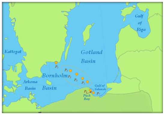

Figure 2.
Baltic Sea regions with marked hydro-meteorological data’s measuring points P1–P7.
The hydro–meteorological change processes at these points were marked as HM(t), t ≥ 0. The same two hydro–meteorological parameters were distinguished for all analyzed processes: the wind speed (in meters per seconds) and the wave height (in meters). There were distinguished w = 6 hydro–meteorological states, and their definitions are presented in Figure 3.

Figure 3.
Fixed states of the hydro–meteorological process.
Hydro–meteorological data collection was created as seven spreadsheets (one for each measuring point). They contain four columns, including a date, an hour, a measuring point’s name, and the hydro–meteorological state in which the measuring time was analyzed. The data were collected over a 6-year period with a 3 h interval between subsequent measurements. The exemplary raw statistical data for Gdynia Port area are shown in Figure 4.
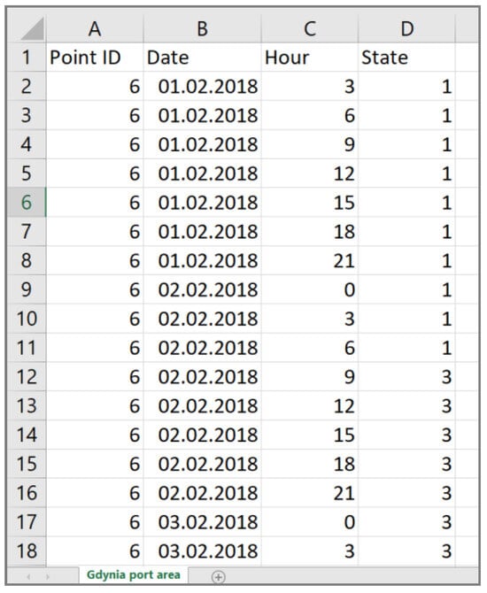
Figure 4.
Exemplary statistical hydro–meteorological data for the Gdynia Port area.
The forecast of hydro–meteorological change was prepared in four cases: separately for three months (December, January, and February) and jointly for winter. To demonstrate how to properly perform the procedure from Section 3, there is a detailed forecast presented for the Puck Bay area during winter. The procedure was implemented in the R language (R-4.3.3 is available for free download from the website https://cran.r-project.org/bin/windows/base/) using the RStudio editor (https://posit.co/download/rstudio-desktop/), and with its help, the forecast was made for considered parts of the Baltic Sea.
First of all, the data were divided into separate datasets. The total number of realizations (fixed as the number of considered days) is n(0) = 480. The number of datasets of the hydro–meteorological change process realizations in which the first taken state was hmb, b = 1, 2, …, 6 are given in the following vector:
[nb(0)]1×6 = [290, 157, 4, 0, 12, 17].
Then, after using (1), the probabilities qb(0), b = 1, 2, …, 6 of the hydro–meteorological change process, taking the hydro–meteorological state hmb at the beginning moment t = 0, are presented in the vector below:
[qb(0)]1×6 = [0.605, 0.327, 0.008, 0, 0.025, 0.035].
The number nbl, b, l = 1, 2, …, 6 of transitions from the state hmb into the state hml in all analyzed datasets of the hydro–meteorological change process realizations are as follows:
The numbers nb, b = 1, 2, …, 6 of the process leaving the hydro–meteorological state hmb are represented by the sums of the rows existing in (9), and given as follows: Taking this into account and applying (3) to (9), the probabilities qbl, b, l = 1, 2, …, 6 of the hydro–meteorological change process transitions from the state hmb to the state hml are shown below:
On the basis of all realizations of the conditional sojourn time HMbl, b, l = 1, 2, …, w of the hydro–meteorological process in the state hmb when the next taken state is hml were fitted distribution functions of conditional sojourn times. They are presented in Table 1 and in Appendix A (Figure A1).

Table 1.
Distribution functions of conditional sojourn times.
A fragment of the source code containing the conformity test is shown in Figure 5. The prediction characteristics of the hydro–meteorological change process starts with the evaluation of the mean values Mb, b = 1, 2, …, 6 of the unconditional sojourn time HMb. They are obtained using (4), with probabilities from (10) and the mean values from Table 1, and are shown in the following vector:
[Mb]1×6 = [96.23, 18.96, 4.46, 0, 4.88, 11.55].
Next, the steady probabilities πb, b = 1, 2, …, 6, received as results of (5), are presented below:
[πb]1×6 = [0.315, 0.42, 0.084, 0, 0.105, 0.076].
Finally, the limit values qb, b = 1, 2, …, 6 of transient probabilities P(HM(t) = hmb), t ≥ 0, b = 1, 2, …, 6 evaluated according to (6) are as follows:
[qb]1×6 = [0.757, 0.199, 0.009, 0, 0.013, 0.022].
It can be concluded that the process stays in the first two states hm1 and hm2 for most of the time, while the chances of the process being in the remaining states hm3–hm6 are marginal (less than 5%). It indicates that the chances of the wave height exceeding 5 m and the wind speed surpassing 17 m/s are estimated to be 4% during winter in the Puck Bay area.
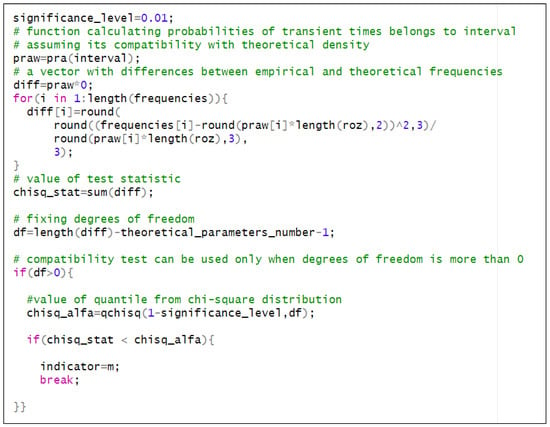

Figure 5.
A fragment of the source code—the conformity test.
The received values of transient probabilities qb, b = 1, 2, …, 6 related to December, January, February, and winter for all considered areas (Karlskrona Port area, Baltic Sea open waters area, Puck Bay area, Gdynia Port area) could be used as the forecast of hydro–meteorological change at the Southern Baltic Sea. They are shown in Figure 6.
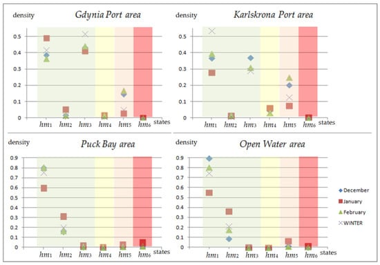
Figure 6.
The forecast of hydro–meteorological changes in the examined areas.
4.2. Discussion of Results
The following main results concerning the prognosis of hydro–meteorological conditions in the southern Baltic Sea during winter were obtained on the basis of the following data contained in Figure 6:
- The relative frequencies of analyzed hydro–meteorological condition occurrence in December and February in all considered areas are very similar; however, the values in January are much different from them;
- The relative frequencies for the Puck Bay area and open water area are very close to each other.
Moreover, dominant hydro–meteorological states for port areas are hm1 and hm3 states corresponding to slow wind speed (less than 17 m/s) and small or high wave height (less than 2 m—hm1 state; more than 5 m—hm3 state). Less likely than them but still noticeable is the state hm5 with fast wind speed (more than 17 m/s) and median wave height (between 2 m and 5 m). The possible reasons for this are various physical and geographical factors; e.g., resonance effects, wave diffraction by breakwaters, tidal changes, wave reflections, and seafloor topography, which can amplify or diminish wave heights. Additionally, weather conditions can significantly affect wave size, leading to extremes rather than average wave heights. These diverse environmental and physical conditions mean wave heights in ports can vary widely, often showing high or low extremes instead of moderate levels.
The dominant hydro–meteorological states for the Puck Bay and open water areas are hm1 and hm2, corresponding to slow wind speed (less than 17 m/s) and small or medium wave high (less than 2 m—hm1 state, with the highest probability; more than 5 m—hm2 state, with the second highest probability), while state hm5 with fast wind speed (more than 17 m/s) and median wave height (between 2 m and 5 m) occurs rarely.
Those facts, supported by the independence test shown in Figure 7, show that wave height and wind speed are dependent on each other.
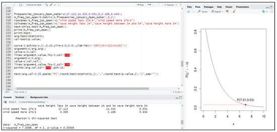
Figure 7.
Chi-square test for independence between wave height and wind speed in open water area during January; performed in RStudio.
Furthermore, using the total probability formula, it is possible to calculate separately only the wave height and the wind speed relative frequencies in each considered range of values, as presented in Figure 8. As we can see in the figure, the relative frequencies of occurrence of high wind speed (more than 17 m/s) are very small in all analyzed areas. The higher the wave, the less frequent it occurs in the areas far away from land (Puck Bay and pen water areas) and the frequency of low and high wave concurrencies are similar in port areas with a smaller frequency medium waves occurring (from 2 to 5 m), as mentioned in the discussion about Figure 6.
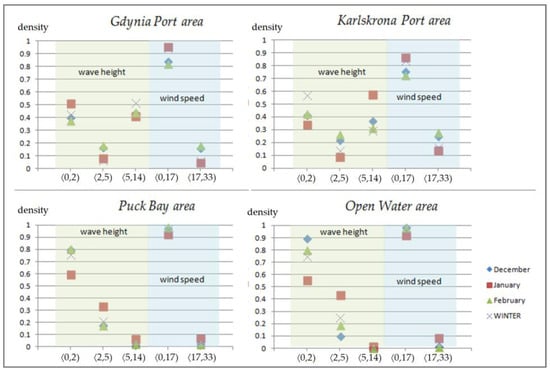
Figure 8.
The forecast of hydro–meteorological change in the southern Baltic Sea area.
This forecast could be used for a safety analysis of shipping critical infrastructure-performing tasks in the Baltic Sea area; e.g., the Stena Line ferry carrying passengers or container ships operating in this region. Conditions considered dangerous to their safety include wind speeds exceeding 17 m/s, which are worse when the waves are high. According to evaluated relative frequencies, the dangerous conditions occur most often in February for port areas and in January for Puck Bay and open water areas. This fact indicates that December is the safest month in winter for critical infrastructure related to the abovementioned parts of the Baltic Sea.
The validation of the created model was conducted using source code written in the R programming language. The empirical relative frequencies of the hydro–meteorological process remaining in their specific states during particular months of the analyzed years were determined. These were compared with predicted frequencies assessed for separate months based on data from previous years. The important part of the code (responsible for calculating empirical relative frequencies) is presented in Figure 9.
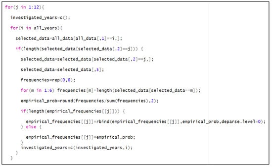
Figure 9.
The part of the model’s source code created in RStudio.
The comparison of empirical and predicted values of occurring hydro–meteorological probabilities in the open waters of the Baltic Sea for selected months is depicted in Figure 10, Figure 11, Figure 12 and Figure 13. It is evident that for data from April, the empirical (colorful points) and predicted probabilities (black asterisks) are very close to each other. In other cases (January, March, and November), significant differences are observed in one of the years. However, these discrepancies can be attributed to the fact that the empirical relative frequencies in that particular year significantly deviate from those of previous years. This validates the methodology and confirms the utility of the model.
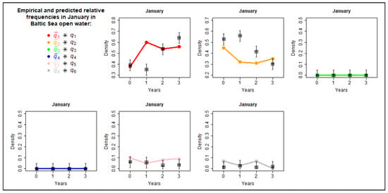
Figure 10.
Empirical and predicted values of occurring hydro–meteorological probabilities in the open waters of the Baltic Sea for January.
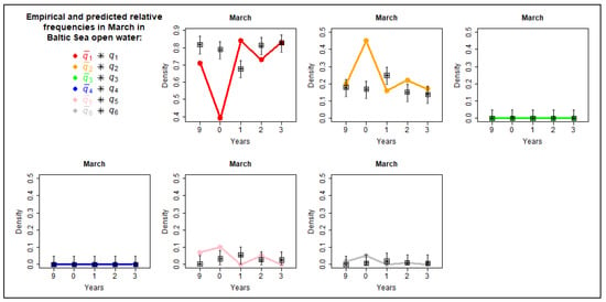
Figure 11.
Empirical and predicted values of occurring hydro–meteorological probabilities in the open waters of the Baltic Sea for March.
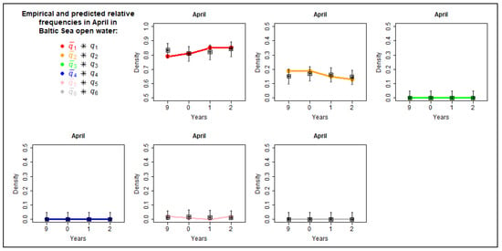
Figure 12.
Empirical and predicted values of occurring hydro–meteorological probabilities in the open waters of the Baltic Sea for April.
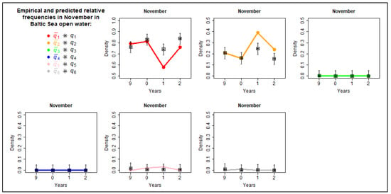
Figure 13.
Empirical and predicted values of occurring hydro–meteorological probabilities in the open waters of the Baltic Sea for November.
There are future plans to expand forecasting in other areas of the Baltic Sea. Through this expansion, it is hoped that customized conservation efforts can be more effectively planned and implemented, addressing the specific needs of each area within the basin.
4.3. Adaptive Strategies within Integrated Coastal Zone Management
Adaptive strategies are essential for mitigating the influence of climate change on the Baltic Sea, as it is particularly susceptible to those impacts. The Helsinki Commission (HELCOM) plays a pivotal role in this regard, serving as a platform for collaboration on environmental protection in this region and supporting research and monitoring. Participatory approaches in decision-making, including stakeholder consultations and community-based management, can enhance the legitimacy and effectiveness of conservation efforts.
The Baltic Sea confronts several multifaceted environmental challenges, including significant pollution loads, eutrophication, biodiversity loss, and the impacts of climate change [41]. The influence of wind exacerbates these issues by affecting the sea’s hydrodynamics and contributing to the complexity of its environmental conditions. The integrated coastal zone management strategies should prioritize the reduction of nutrient runoff, sustainable fishery management, pollution control, and restoration of habitats, such as seagrass meadows and wetlands, to enhance ecosystems’ biodiversity [41]. Efforts should focus on harmonizing policies, sharing best practices, and engaging in joint monitoring and research initiatives.
Waves play a significant role in the transport and dispersion of nutrient runoff in the Baltic Sea. Waves can cause erosion along coastlines and riverbanks, especially during storms or periods of high wave energy [42]. This erosion can dislodge soil particles and organic matter containing nutrients, such as nitrogen and phosphorus, and transport them into the water. The nutrients that have settled on the seabed can be resuspended into the water column by wave action. This resuspension of sediments occurs when waves disturb the sediment layer, releasing nutrients back into the water where they can be transported to other areas. The transport of nutrients can contribute to their dispersion over larger spatial scales, potentially impacting ecosystems beyond coastal regions. Increased nutrient runoff due to human activities can lead to eutrophication, which, in turn, leads to the accelerated growth of algae and aquatic plants [43]. High-energy waves, particularly during storm events, can cause physical damage to coastal ecosystems, such as seagrass beds and salt marshes. This damage can disrupt habitats and ecosystems that play important roles in nutrient cycling, sedimentation, denitrification, nutrient uptake by primary producers, and water quality regulation.
To protect coastal zones from the dynamic and potentially destructive influences of combined wind and wave impacts, the construction of physical barriers to absorb and deflect the energy of wind-driven waves can be built, thereby reducing erosion and protecting inland areas [42]. In the Gulf of Gdansk in the Gdynia Orlowo region, there is a cliff that is experiencing erosion, thereby diminishing its touristic appeal [44]. Another strategy is the restoration and conservation of natural barriers such as mangroves and dunes, which serve as buffers against wind and wave action, trapping sediments and stabilizing shorelines naturally. Moreover, there is a need for implementing advanced forecasting and early warning systems for extreme weather events.
Enhancing the resilience of infrastructure and improving emergency preparedness are crucial measures to effectively cope with natural hazards. Adaptation strategies should promote climate-smart maritime and coastal infrastructure that can withstand extreme weather events, such as stronger storms. Existing models for forecasting in the safety analysis of maritime infrastructures, e.g. referenced in [17,45], are planned for real-case application. Expanding the model introduced in this paper to include inland water bodies will not only improve water system safety models [46] but also allow adaptation to various environments, enhancing critical infrastructure operations by integrating variable hydro-meteorological conditions, e.g. to Refs. [18,47]. To effectively combat pollution, adaptation strategies must be tailored to fluctuating hydro–meteorological conditions [17,45]. Weather forecasts play a crucial role in anticipating the dispersion patterns of pollutants, enabling proactive measures such as adjusting waste management practices accordingly. Leveraging the forecasting model presented in this paper for simulating oil discharge trajectories [1,34] provides valuable insights into the potential spread of contaminants.
5. Conclusions
This paper presents forecasts and trends in hydro–meteorological parameters for the southern Baltic Sea by applying a detailed procedure, which can be extended to other maritime regions. The obtained forecast of these parameters turned out to be consistent with the description contained and validated previously in this article, which confirms the correctness of the created procedure. This allows for future plans to expand the analysis to other parts of the Baltic Sea or other open water areas and to use the obtained predictions to analyze the safety of critical water infrastructure and mitigate the effects of exposure of this infrastructure to dangerous values of the factors discussed. However, despite the advantages, there exist certain limitations.
First, we assume that the hydro–meteorological change process is a periodic semi-Markov process and, given the changing climate, it may not take into account the natural variability of the marine environment. Moreover, if the number of realizations of the transition time between states is greater than 30, a theoretical distribution has been assigned. Of all the fitted distributions, the best was selected for the p-value from the chi-square goodness-of-fit test. Furthermore, the states should be defined in an appropriate way so that the number of transitions from one state to the next is as high as possible. Otherwise, it will be difficult to fit the theoretical distribution. In the future, it may turn out that taking into account a larger number of realizations, we can obtain a different forecast.
The data used in the model originate from measurement buoys, thereby eliminating the potential for human error as they are processed by a machine. The model possesses the capacity for future modifications; for instance, if the data transmission is human-mediated, adjustments can be made to the algorithm to effectively identify and mitigate outlier values, such as unusually high temperatures recorded in January, by either removing or substituting them with more representative data points.
Author Contributions
Conceptualization, E.D. and M.T.; methodology, E.D. and M.T.; software, M.T.; validation, M.T.; formal analysis, E.D. and M.T.; investigation, M.T.; resources, E.D. and M.T.; data curation, E.D. and M.T.; writing—original draft preparation, M.T. and E.D.; writing—review and editing, M.T. and E.D.; visualization, E.D. and M.T.; supervision, E.D. and M.T. All authors have read and agreed to the published version of the manuscript.
Funding
This research was funded from the statutory activities of Gdynia Maritime University, grant number WN/PI/2024/03: “The influence of the oil layer thickness and the hydro-meteorological changes process on the movement of oil spills at sea”.
Data Availability Statement
The data presented in this study are available upon request from the authors, excluding some data protected by copyright.
Conflicts of Interest
The authors declare no conflicts of interest.
Appendix A
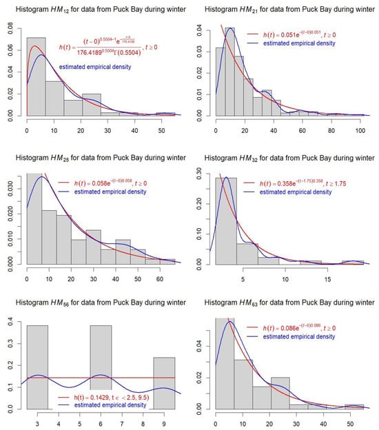
Figure A1.
Histograms with theoretical and empirical densities for sojourn times in the Puck Bay area during winter.
References
- Dąbrowska, E. Oil discharge trajectory simulation at selected Baltic Sea waterway under variability of hydro-meteorological conditions. Water 2023, 15, 1957. [Google Scholar] [CrossRef]
- Bogalecka, M. Consequences of Maritime Critical Infrastructure Accidents. Environmental Impacts Modeling—Identification—Prediction—Optimization—Mitigation; Elsevier: Amsterdam, The Netherlands, 2020. [Google Scholar] [CrossRef]
- Pliemon, T.; Foelsche, U.; Rohr, C.; Pfister, C. Subdaily meteorological measurements of temperature, direction of the movement of the clouds, and cloud cover in the Late Maunder Minimum by Louis Morin in Paris. Clim. Past 2022, 18, 1685–1707. [Google Scholar] [CrossRef]
- Pankina, S.I.; Tsepordey, O.V.; Kravchenko, A.I.; Somko, M.L.; Lyutikova, M.N. An assessment model of exposure on coastal zone ecosystems. IOP Conf. Ser. Earth Environ. Sci. 2021, 872, 012016. [Google Scholar] [CrossRef]
- Ullman, D.S.; Ginis, I.; Huang, W.; Nowakowski, C.; Chen, X.; Stempel, P. Assessing the Multiple Impacts of Extreme Hurricanes in Southern New England, USA. Geosciences 2019, 9, 265. [Google Scholar] [CrossRef]
- Kerimoglu, O.; Voynova, Y.G.; Chegini, F.; Brix, H.; Callies, U.; Hofmeister, R.; Klingbeil, K.; Schrum, C.; van Beusekom, J.E.E. Interactive impacts of meteorological and hydrological conditions on the physical and biogeochemical structure of a coastal system. Biogeosciences 2020, 17, 5097–5127. [Google Scholar] [CrossRef]
- Iz, H. The effect of regional sea level atmospheric pressure on sea level variations at globally distributed tide gauge stations with long records. J. Geod. Sci. 2018, 8, 55–71. [Google Scholar] [CrossRef]
- Gurova, E.; Lehmann, A.; Ivanov, A. Upwelling dynamics in the Baltic Sea studied by a combined SAR/infrared satellite data and circulation model analysis. Oceanologia 2013, 55, 687–707, ISSN 0078-3234. [Google Scholar] [CrossRef]
- Meier, H.E.M.; Kniebusch, M.; Dieterich, C.; Gröger, M.; Zorita, E.; Elmgren, R.; Myrberg, K.; Ahola, M.P.; Bartosova, A.; Bonsdorff, E.; et al. Climate change in the Baltic Sea region: A summary. Earth Syst. Dynam. 2022, 13, 457–593. [Google Scholar] [CrossRef]
- Harris, S.A. Comparison of Recently Proposed Causes of Climate Change. Atmosphere 2023, 14, 1244. [Google Scholar] [CrossRef]
- Venegas, R.M.; Acevedo, J.; Treml, E.A. Three decades of ocean warming impacts on marine ecosystems: A review and perspective. Deep Sea Res. Part II Top. Stud. Oceanogr. 2023, 212, 105318, ISSN 0967-0645. [Google Scholar] [CrossRef]
- Debele, S.E.; Kumar, P.; Sahani, J.; Marti-Cardona, B.; Mickovski, S.B.; Leo, L.S.; Porcù, F.; Bertini, F.; Montesi, D.; Vojinovic, Z.; et al. Nature-based solutions for hydro-meteorological hazards: Revised concepts, classification schemes and databases. Environ. Res. 2019, 179, 108799, ISSN 0013-9351. [Google Scholar] [CrossRef] [PubMed]
- Lewis, N.T.; Seviour, W.J.M.; Roberts-Straw, H.E.; Screen, J.A. The response of surface temperature persistence to Arctic sea-ice loss. Geophys. Res. Lett. 2024, 51, e2023GL106863. [Google Scholar] [CrossRef]
- Röthig, T.; Trevathan-Tackett, S.M.; Voolstra, C.R.; Ross, C.; Chaffron, S.; Durack, P.J.; Warmuth, L.M.; Sweet, M. Human-induced salinity changes impact marine organisms and ecosystems. Glob. Change Biol. 2023, 29, 4731–4749. [Google Scholar] [CrossRef] [PubMed]
- HELCOM. Baltic Sea Action Plan—2021 Update; HELCOM: Helsinki, Finland, 2021. [Google Scholar]
- Pompei, C.; Alves, E.; Vieira, E.; Campos, L. Impact of meteorological variables on water quality parameters of a reservoir and ecological filtration system. Int. J. Environ. Sci. Technol. 2019, 17, 1387–1396. [Google Scholar] [CrossRef]
- Kołowrocki, K.; Kuligowska, E.; Soszyńska-Budny, J.; Torbicki, M. An Approach to Safety Prediction of Critical Infrastructure Impacted by Climate-Weather Change Process. In Proceedings of the International Conference on Information and Digital Technologies 2017-IDT, Zilina, Slovakia, 5–7 July 2017; pp. 183–186, ISBN 978-1-5090-5688-0. ISSN 2585-7614. [Google Scholar]
- Magryta-Mut, B. Modeling safety of port and maritime transportation systems. Sci. J. Marit. Univ. Szczec. 2023, 74, 65–74. [Google Scholar] [CrossRef]
- Jaseena, K.U.; Kovoor, B.C. Deterministic weather forecasting models based on intelligent predictors: A survey. J. King Saud Univ. Comput. Inf. Sci. 2022, 34, 3393–3412, ISSN 1319-1578. [Google Scholar] [CrossRef]
- Palmer, T.N. Stochastic weather and climate models. Nat. Rev. Phys. 2019, 1, 463–471. [Google Scholar] [CrossRef]
- Kołowrocki, K.; Soszyńska-Budny, J. Reliability and Safety of Complex Technical Systems and Processes: Modeling—Identification—Prediction—Optimization, 1st ed.; Springer: London, UK, 2011. [Google Scholar]
- Torbicki, M. Longtime Prediction of Climate-Weather Change Influence on Critical Infrastructure Safety and Resilience. In Proceedings of the 2018 IEEE International Conference on Industrial Engineering and Engineering Management (IEEM), Bangkok, Thailand, 16–19 December 2018; pp. 996–1000. [Google Scholar] [CrossRef]
- Jakusik, E. The Impact of Climate Change on the Characteristics of the Wave in the Southern Part of the Baltic Sea and Its Consequences for the Polish Coastal Zone. Ph.D. Thesis, IMGW-PIB, Marine Research Department, Warsaw, Poland, 2012. [Google Scholar]
- WMO. The Climate of the Baltic Sea; Report WMO/TD-No. 933; WMO: Geneva, Switzerland, 1993. [Google Scholar]
- BACC II. Second Assessment of Climate Change for the Baltic Sea Basin. In The BACC II Author Team (Red.); Springer: London, UK, 2015. [Google Scholar]
- Shestakova, A.A.; Repina, I.A. Overview of strong winds on the coasts of the Russian Arctic seas. Ecol. Montenegrina 2019, 25, 14–25. [Google Scholar] [CrossRef]
- Dobrzycka-Krahel, A.; Bogalecka, M. The Baltic Sea under Anthropopressure—The Sea of Paradoxes. Water 2022, 14, 3772. [Google Scholar] [CrossRef]
- Bogalecka, M. Consequences of maritime critical infrastructure accidents with chemical releases. Int. J. Mar. Navig. Saf. Sea Transp. 2019, 13, 771–779. [Google Scholar] [CrossRef]
- Jakusik, E.; Kołowrocki, K.; Kuligowska, E.; Soszyńska-Budny, J. Identification of climate related hazards at the Baltic Sea area. J. Pol. Saf. Reliab. Assoc. Summer Saf. Reliab. Semin. 2016, 7, 99–104. [Google Scholar]
- Zalewska, T.; Jakusik, E. Warunki Meteorologiczne i Hydrologiczne Oraz Charakterystyka Elementów Fizycznych, Chemicznych i Biologicznych Południowego Bałtyku w 2018 Roku. Available online: https://www.imgw.pl/sites/default/files/2020-08/imgw-baltyk-monografia_final.pdf (accessed on 2 April 2024).
- Soomere, T.; Weisse, R.; Behrens, A. Wave climate in the Arkona Basin, the Baltic Sea. Ocean Sci. 2012, 8, 287–300. [Google Scholar] [CrossRef]
- HELCOM. Climate Change in the Baltic Sea Area. In Baltic Sea Environment Proceedings; HELCOM: Helsinki, Finland, 2007; Volume 111. [Google Scholar]
- Admiralty Sailing Directions—Baltic Pilot. 2001. 1, Baltic Master Report M II part 2/4. In General Assumptions of the Ship Safety on Southern and Western Baltic Sea; Maritime University of Szczecin: Szczecin, Poland, 2007.
- Dąbrowska, E. Numerical Modelling and Prediction of Oil Slick Dispersion and Horizontal Movement at Bornholm Basin in Baltic Sea. Water 2024, 16, 1088. [Google Scholar] [CrossRef]
- HELCOM. Climate change in the Baltic Sea Area—HELCOM thematic assessment in 2013. In Baltic Sea Environment Proceedings; HELCOM: Helsinki, Finland, 2013; Volume 137. [Google Scholar]
- Fammler, H.; Weber, H.S.; Fawzy, T.; Kuris, M.; Remmelgas, L.; Veidemane, K.; Bryan, T.; Johansen, K.S.; Piwowarczyk, J. The Story of Eutrophication and Agriculture of the Baltic Sea. Available online: https://www.responseable.eu/wp-content/uploads/key-story-eutrophication-0518.pdf (accessed on 2 April 2024).
- Barbariol, F.; Davison, S.; Falcieri, F.M.; Ferretti, R.; Ricchi, A.; Sclavo, M.; Benetazzo, A. Wind Waves in the Mediterranean Sea: An ERA5 Reanalysis Wind-Based Climatology. Front. Mar. Sci. 2021, 8, 760614. [Google Scholar] [CrossRef]
- Chérubin, L.M.; Garavelli, L. Eastern Caribbean Circulation and Island Mass Effect on St. Croix, US Virgin Islands: A Mechanism for Relatively Consistent Recruitment Patterns. PLoS ONE 2016, 11, e0150409. [Google Scholar] [CrossRef]
- Jensen, J.; Dangendorf, S.; Wahl, T.; Steffen, H. Sea level changes in the North Sea region: Recent developments and future challenges with focus on the German Bight. Hydrol. Wasserbewirtsch. 2014, 58, 304–323. [Google Scholar]
- Kuligowska, E.; Torbicki, M. Climate-weather change process realizations uniformity testing for maritime ferry operating area. In Proceedings of the 17th ASMDA Conference Proceedings, Applied Stochastic Models and Data Analysis, London, UK, 6–9 June 2017; pp. 605–620. [Google Scholar]
- HELCOM. State of the Baltic Sea. Third HELCOM holistic assessment 2016–2021. In Baltic Sea Environment Proceedings; HELCOM: Helsinki, Finland, 2023; Volume 194, ISSN 0357-2994. [Google Scholar]
- Ostrowski, R.; Pruszak, Z.; Babakov, A. Condition of South-Eastern Baltic Sea Shores and Methods of Protecting Them. Arch. Hydro-Eng. Environ. Mech. 2015, 61, 17–37. [Google Scholar] [CrossRef]
- Akinnawo, S.O. Eutrophication: Causes, consequences, physical, chemical and biological techniques for mitigation strategies. Environ. Chall. 2023, 12, 100733, ISSN 2667-0100. [Google Scholar] [CrossRef]
- Bełdowska, M.; Bełdowski, J.; Kwasigroch, U.; Szubska, M.; Jędruch, A. Coastal cliff erosion as a source of toxic, essential and nonessential metals in the marine environment. Oceanologia 2022, 64, 553–566. [Google Scholar] [CrossRef]
- Kołowrocki, K.; Kuligowska, E.; Soszyńska-Budny, J.; Torbicki, M. Safety and Risk Prediction of Port Oil Piping Transportation System Impacted by Climate-Weather Change Process. In Proceedings of the International Conference on Information and Digital Technologies 2017-IDT 2017, Zilina, Slovakia, 5–7 July 2017; pp. 173–177, ISBN 978-1-5090-5688-0. [Google Scholar]
- Pietrucha-Urbanik, K.; Żelazko, A. Approaches to assess water distribution failure. Period. Polytech. Civ. Eng. 2017, 61, 632–639. [Google Scholar] [CrossRef]
- Woch, M.; Zieja, M.; Tomaszewska, J. Analysis of the Time between Failures of Aircrafts. In Proceedings of the 2nd International Conference on System Reliability and Safety (ICSRS), Milan, Italy, 20–22 December 2017; pp. 112–118. [Google Scholar] [CrossRef]
Disclaimer/Publisher’s Note: The statements, opinions and data contained in all publications are solely those of the individual author(s) and contributor(s) and not of MDPI and/or the editor(s). MDPI and/or the editor(s) disclaim responsibility for any injury to people or property resulting from any ideas, methods, instructions or products referred to in the content. |
© 2024 by the authors. Licensee MDPI, Basel, Switzerland. This article is an open access article distributed under the terms and conditions of the Creative Commons Attribution (CC BY) license (https://creativecommons.org/licenses/by/4.0/).