An Application of the RegCM4 System to Quantify the Effects of Climate Change on the Hydric Potential of the Angostura-Bolivia Basin

Abstract

Climate change (CC) impacts on hydrology pose significant global concerns due to their effects on water availability, thereby impacting various human activities reliant on this essential resource. This study assesses the influence of CC on the water supply in the Angostura-Bolivia basin. We employed the RegCM4 system, which develops its own regional climate models (RCMs) tailored to the Angostura basin using specific convective schemes, diverging from reliance on pre-existing RCMs, like those provided by CORDEX. Methodologically, the study involves hydrometeorological data collection and analysis, utilizing dynamic and statistical downscaling methods to refine the RCMs derived from ERA-Interim reanalysis data. Subsequently, precipitation and temperature projections are generated under CC scenarios (RCP 4.5 and RCP 8.5) for both near (2045–2055) and far (2065–2075) future periods, compared to the historical period (1981–2010). The final stage employs the HydroBID system to project future runoff, considering both perturbed and unperturbed hydrometeorological data under CC effects. The analysis of flow duration curves for 50%, 75%, and 90% exceedance probabilities reveals a significant reduction in flows across all scenarios, indicating a noteworthy impact on water availability. These findings underscore the urgency of comprehending and adapting to CC on hydrology, emphasizing the critical importance of sustainable water resource management amidst evolving climatic conditions.

1. Introduction

Greenhouse gas emissions have increased since pre-industrial times, and they are now higher than ever [1]. Hence, continued emission of these gases will cause irreversible changes in the components of the climate system, including an increase in the occurrence of extreme events related to temperatures and precipitation [2].

Aiguo Dai concludes that, on a global scale, droughts will be more frequent in future years [3]. Under these conditions, studies of the potential impacts that climate change (CC) may have on water resources would become indispensable for the future, especially when it comes to large-scale projects, by incorporating appropriate management to minimize adverse effects [4].

Climate and Earth models are our main tools for projecting future climate [5,6]. The typical resolution of global climate models (GCMs) is 100–300 km [7]. This resolution cannot adequately represent orography, land cover, and atmospheric dynamics, hindering their ability to simulate climate events and extreme weather [8].

Studies performed by Aldunate Lipa quantified the effects of CC on the water potential of a pilot basin [9], through the use of regional climate models (RCMs) [10] generated by CORDEX [11,12], located in the Department of Santa Cruz-Bolivia. Those studies found changes in the temporal distribution of precipitation during a hydrological year, with less water for the dry months and more precipitation during the rainy season; at the time of the quantification of these effects, an essential variation in the extent of the results was seen, an aspect that shows a notorious uncertainty when looking for factors to guide the effects of CC in the design of engineering works related to our area of interest [13]. On the other hand, research conducted on future changes in the Yangtze River basin, China, through statistical downscaling has concluded that such methods are effective measures for bridging the gap between large-scale climate change and local-scale hydrological responses [14]. Similarly, the Quantile Delta Mapping technique has been tested in other basins [15].

Therefore, this paper argues how to quantify the effects of CC at the basin scale through techniques also known as downscaling in order to improve the resolution of RCMs [16] and quantify such effects on the hydric potential based on self-generated RCMs from the RegCM4.0 system, in order for decision makers in charge of water resources to be able to rely on estimates of CC impacts for a reasonable time period [17]. However, this is based on the fact that the adequate representation of the present climate implies a better performance when representing the future climate under climate change scenarios.

2. Materials and Methods

In Figure 1, a flowchart is presented, summarizing the methodology to be followed in this paper.

2.1. Study Area and Hydrometeorological Data

2.1.1. Study Area

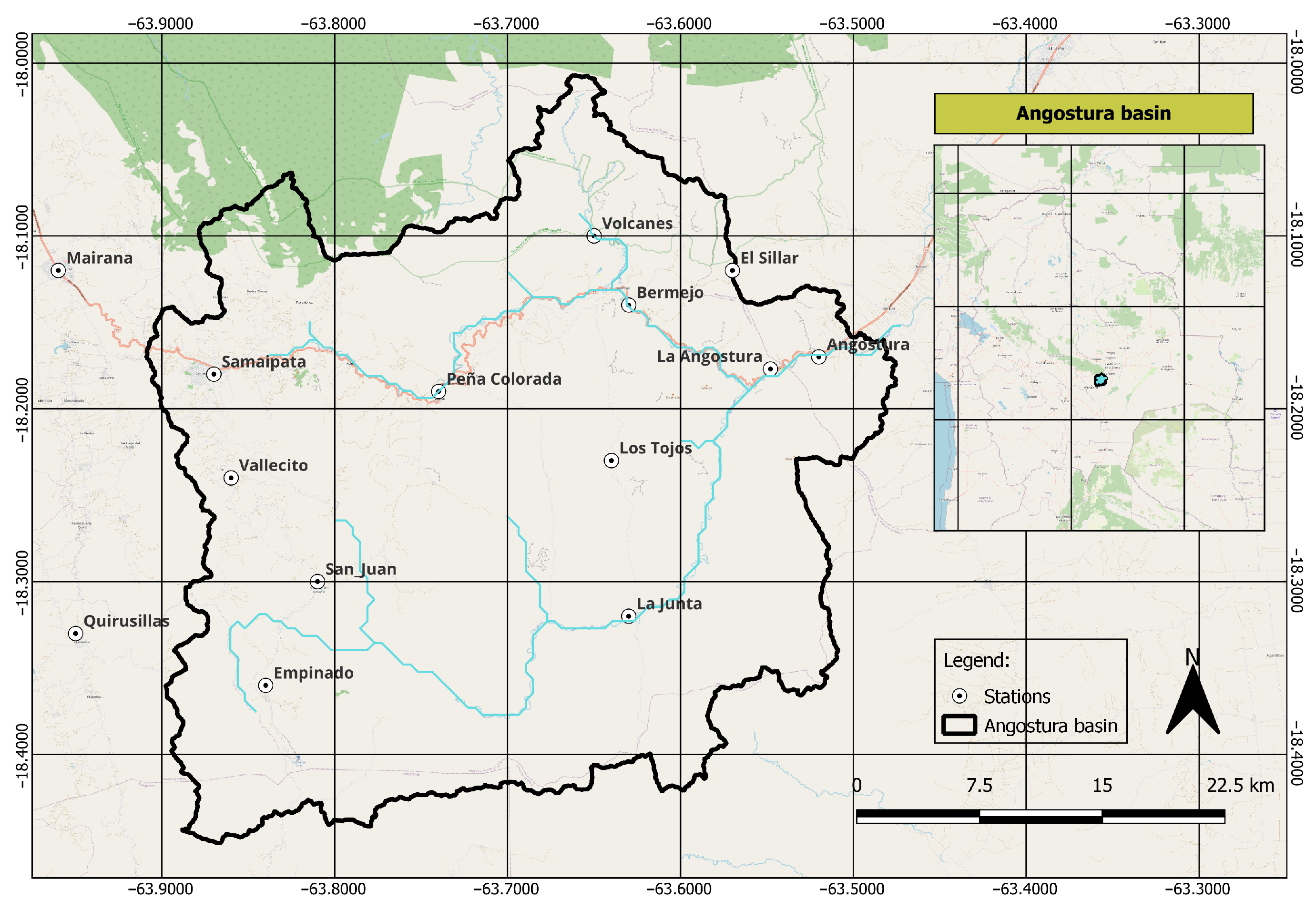
The study area, called Angostura basin, is part of the hydrographic basin of the Piraí River, which is a tributary of the Grande River that flows into the Mamoré River and then joins the Amazon River. In particular, the study basin corresponds to the upper Piraí River basin, which is located in the sub-Andean belt of the Santa Cruz department (Bolivia).

The Angostura basin has its headwaters in the mountainous part of the town of Samaipata, flowing into the area next to the La Angostura hydrometric station. The basin covers an area of approximately 1454.6 km².

The geographic coordinates bounding the basin correspond to 63.910° to 63.475° west longitude and 18.450° to 18.005° south latitude, as shown in Figure 2.

For the delimitation of the Angostura basin, we opted to work with a digital elevation model (DEM) of the terrain obtained from the GeoBolivia website https://geo.gob.bo (accessed on 26 January 2022). This DEM is in GeoTIFF format with lat/long geographic coordinates and has a spatial resolution of 30 m.

The soil type representation for the basin was sourced from the Food and Agriculture Organization of the United Nations (FAO) [18], accessible through the Centro Digital de Recursos Naturales de Bolivia platform. According to these data, the study area exhibits a predominance of Lithosols, Chromic Luvisols, and Cambisols, in particular on mountainous slopes.

According to the AHD-HydroBID data, the highest percentage of cover in the area is attributed to evergreen needle-leaf forest, accounting for 76.6%. This is followed by deciduous needle-leaf forest. Additionally, irrigated agricultural lands and pastures make up a minimal proportion, only 0.1%, alongside shrub forests, which are also present in smaller proportions.

2.1.2. Hydrometeorological Data

The records of daily accumulated precipitation [mm], the average daily temperature in °C, and daily flow series in m³/s were obtained from 14 rainfall stations (see

Table 1. Description and location of hydrometeorological stations.

N.	Station Name	Latitude	Longitude	Variable	Period
1	Empinado	−18.363	−63.837	Precipitation	1 January 1976–31 December 2012
2	Peña Colorada	−18.191	−63.738	Precipitation	1 January 1976–31 December 2012
3	Bermejo	−18.137	−63.630	Precipitation	1 January 1976–31 December 2012
4	Volcanes	−18.107	−63.652	Precipitation	1 January 1976–31 December 2012
5	Vallecito	−18.240	−63.856	Precipitation	1 January 1976–31 December 2012
6	El sillar	−18.119	−63.568	Precipitation	1 January 1976–31 December 2012
7	Los Tojos	−18.229	−63.668	Precipitation	1 January 1976–31 December 2012
8	Quirusillas	−18.332	−63.945	Precipitation	1 January 1976–31 December 2012
9	La Junta	−18.315	−63.625	Precipitation	1 January 1976–31 December 2012
10	Angostura	−18.165	−63.520	Precipitation	1 January 1976–31 December 2012
11	San Juan	−18.303	−63.810	Precipitation	1 January 1976–31 December 2012
12	Mairana	−18.116	−63.958	Precip/Temp	1 January 1976–31 December 2012
13	Samaipata	−18.176	−63.870	Precipitation	1 January 1976–31 December 2012
14	La Angostura	−18.177	−63.548	Water Flow	1 January 1976–31 December 2012

), the geographical distribution of which is given in Figure 2. The measured daily rainfall for the 30-year period of 01-1981 to 12-2010 was used to assess hydro-climatic variability [5].

The measurement sites have been monitored by the Water Channelling and Regularization Service of the Piraí River (SEARPI) and the National Service of Meteorology and Hydrology (SENAMHI).

Representative precipitation in the Angostura basin was calculated by applying the Thiessen polygon method. These polygons allow us to obtain the desired precipitation based on the weighted average of the stations in and near the basin.

Therefore, Figure 3 summarizes the representative total annual precipitation, with an average value of 1121.0 mm. From 30 years of the base period, 11 years were above average, i.e., 37% of the years had above-average precipitation. Additionally, the precipitation recorded in the hydrological year 1989/1990 (1465 mm) was the highest, while the lowest occurred in the hydrological year 1994/1995, reaching a value of 709 mm.

2.2. Simulated Hydrometeorological Data

2.2.1. Dynamic Downscaling

RCMs have been developed to study regional processes and generate high-resolution physical climate information at scales relevant to Vulnerability, Impact, and Adaptation (VIA) studies [11]. Although these models inherit biases from the initial model, they have the potential to illustrate the interaction effect between large-scale feature changes and complex topographic-scale or urban environments, a process that GCMs fail to simulate [19]. The self-generated RCMs by the RegCM4 system [20] were used, starting from the ERA-Interim [21] reanalysis data, which contain a large variety of surface parameters collected at 3-hourly intervals, describing both land and oceanic conditions [22]. For the basin scale, the RCMs obtained from the Sensit02 and Sensit04 experiments were used.

Table 2. Experiment specifications to generate regional climate models.

Experiments	Spatial Resolution ds (km)	Temporal Resolution dt (s)	Number of Vertical Levels $\mathit{\sigma }$	Convective Scheme on Land (icup_lnd)	Convective Scheme in Ocean (icup_ocn)	Humidity Scheme/ Microphy of Particles	Planetary Boundary Scheme (ibltyp)
Sensit01	30	30	18	Grell (2)	Emmanuel (4)	SUBEX (1)	Holtslag (1)
	10	10	18
	5	5	18
Sensit02	30	30	18	Emmanuel (4)	Grell (2)	SUBEX (1)	Holtslag (1)
	10	10	18				Holtslag (1)
	5	5	23				UW (2)
Sensit03	30	30	18	Tiedke (5)	Tiedke (4)	SUBEX (1)	Holtslag (1)
	10	10	18
	5	5	23
Sensit04	30	30	18	Grell (2)	Kain (6)	SUBEX (1)	Holtslag (1)
	10	10	18
	5	5	23

shows the parameters used for each experiment according to the spatial resolution in km.

Each experiment began with the ERA-Interim reanalysis data to generate an RCM with a resolution of 30 km, then this RCM was taken as a starting point to perform the dynamic downscaling to generate an RCM of 10 km resolution; finally, this new RCM was taken as a starting point to generate the RCM of 5 km by 5 km, which is the resolution we are looking to achieve at the basin scale.

2.2.2. Data Extraction for 5 km RCMs

The data extraction from the generated regional climate models was performed by using 2 methods proposed by Hakala [23] and 1 additional method proposed based on the possibilities of having fine grids with a resolution of 5 km by 5 km.

(a) The first method consists of extracting the data from the grid closest to the basin centroid coordinates; (b) the second method involves taking the average of all grids overlapping across the basin area and (c) obtaining the average of the grids closest to the coordinates of each station within the basin. Hence, it is observed that method (a) with the grid information closest to the basin centroid coordinates is the best performing procedure.

The Sensit04 experiment overestimates precipitation in most months by a large amount (see Figure 4); the same behavior is shown in any of the 3 data-extraction methods. On the other hand, the Sensit02 experiment provides a better representation of the observed data, although the months of January and February are the furthest away from the local data and are a clue for model calibration.

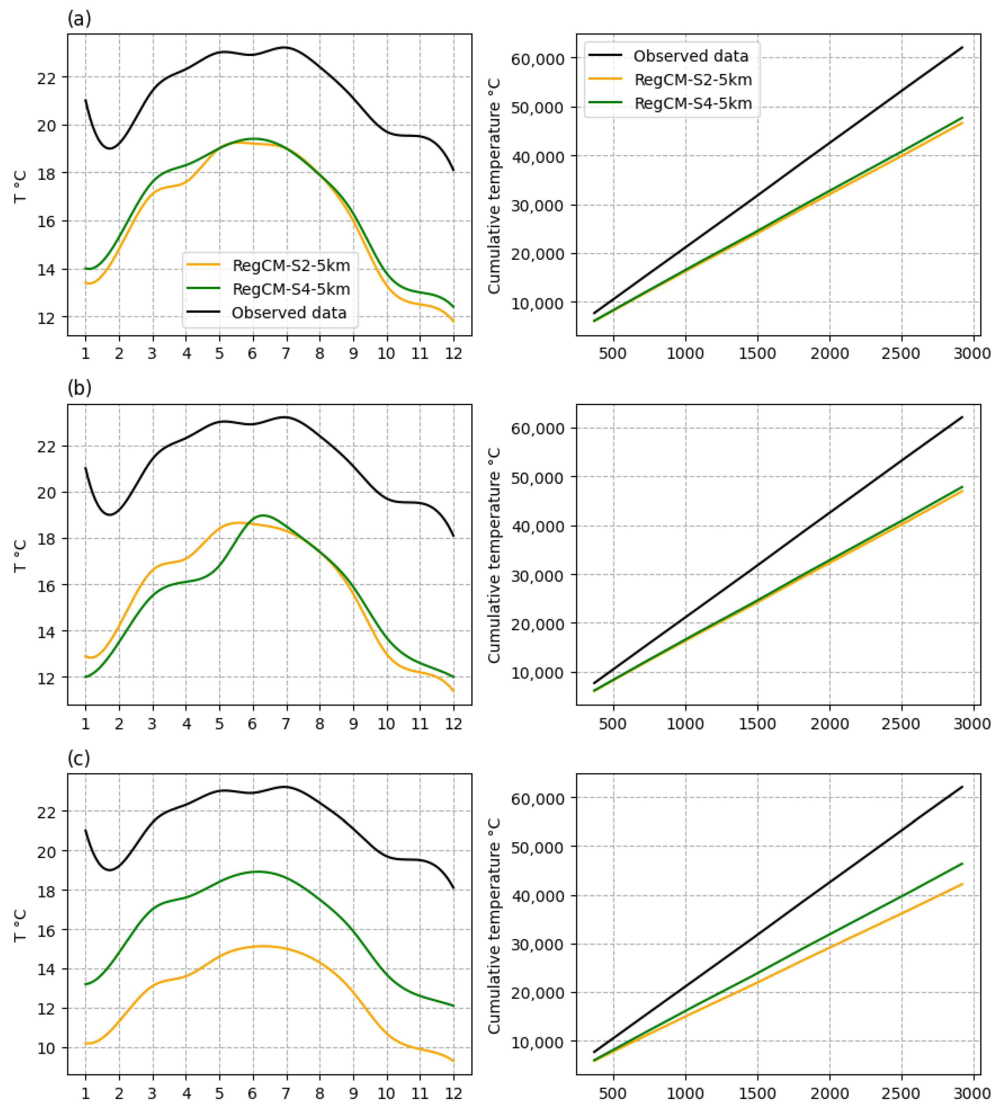
• The modeled temperature in both experiments follows the pattern of the observed temperature (see Figure 5), but with a bias of about 4 °C. On the other hand, the plots reinforce the idea that the extraction method (a) represents the basin in a better way.

2.2.3. Statistical Downscaling

In order to overcome this scale-related gap between what GCMs provide and what hydrological impact modelers need, statistical downscaling methods are traditionally applied to sort out this problem [24].

Statistical downscaling techniques involve developing empirical relationship between long-scale atmospheric variables (the predictors) and local surface variables (the predictands) [25,26], which can be expressed by the equation below.

$$R\backsim F\left(x\right)$$

(1)

Statistical downscaling was applied (see Figure 6) to the regional climate models generated from the Sensit02 and Sensit04 experiment at 10 km resolution for the baseline period.

Quantile Delta Mapping

The Quantile Delta Mapping (QDM) method for precipitation preserves the relative quantile changes of the projected models, while at the same time systematically correcting the quantile uncertainty of the modeled series with respect to the observed values [15].

To apply statistical downscaling (SD), the Quantile Delta Mapping method using parametric transformations [27,28] was chosen, due to its capacity to perform statistical downscaling as such and, at the same time, correct for quantile biases. These transformations can be expressed in terms of the following:

Potential transformation:

$$P_{obs}^{*}=B\ast {\left(P_{mod}\right)}^c$$

(2)

Exponential transformation:

$$P_{obs}^{*}=(A+B\ast P_{mod})\ast (1-e^{\frac{-P_{mod}}{\tau }})$$

(3)

$P_{obs}^{*}$ and $P_{mod}$ are the corrected and uncorrected modeled values, respectively, and $A,B$, and $\tau$ are the free parameters that need to be optimized.

The application of the QDM method to the historical precipitation series data modeled by the Sensit02 and Sensit04 experiments with 10 km resolution can be seen in Figure 6.

Delta-Change Approach

The idea behind the widely used delta-change method is to use the modeled future changes (anomalies) for a perturbation of the observed data instead of the simulation of future conditions from the RCM itself. The control period, also known as the climatological baseline, corresponds then, by definition, to the observed climate and cannot be used for a proper evaluation. Generally, the calculation is made on a monthly basis [29].

Hence, a multiplicative correction is used for precipitation, and an additive correction is used to adjust the temperature, which are represented as follows [29].

$$P_{m,h}^{*}\left(t\right)=P_{o,h}\left(t\right)$$

(4)

$$P_{m,p}^{*}\left(t\right)=P_{o,h}\left(t\right)\left[\frac{{\overline{P}}_{m,p}\left(t\right)}{{\overline{P}}_{m,h}\left(t\right)}\right]$$

(5)

$$T_{m,h}^{*}=T_{o,h}\left(t\right)$$

(6)

$$T_{m,h}^{*}=T_{o,h}\left(t\right)+T_{m,p}^{*}\left(t\right)-{\overline{T}}_{m,h}\left(t\right)$$

(7)

where $P_{m,h}^{*}\left(t\right)$ means modeled historical average precipitation, $P_{o,h}\left(t\right)$ observed historical precipitation, $P_{m,p}^{*}\left(t\right)$ modeled projected average precipitation, $T_{m,h}^{*}$ modeled historical average temperature, $T_{o,h}\left(t\right)$ observed historical temperature, $T_{m,h}^{*}$ modeled historical average temperature, $T_{m,h}$ modeled historical temperature, and $T_{m,p}^{*}\left(t\right)$ modeled projected average temperature.

In order to evaluate the performance of the results obtained from the regional climate models using both downscaling methods, parameters known as precipitation climate metrics were used [30].

2.3. Angostura Basin Projections

2.3.1. Climate Projections

An approximate ensemble of results was considered based on 2 pre-selected RCMs, involving future forcing scenarios RCP 4.5 and 8.5 covering the periods of the 2050s (2045 to 2055) and 2070s (2065 to 2075). These scenarios were adopted due to RCP 4.5 corresponding to the expected future trajectory and RCP 8.5 as a critical trajectory that simulates an increase of the consumption of the fuels considered.

In order to quantify changes in the temperature and precipitation values, we calculated the change signal by comparing projected and historical series. Therefore, we define “change” as the difference between statistical characteristics associated with both variables of interest.

The equation is expressed to calculate the change within projected and historical variables defined as $\Delta P$ and $\Delta T$, respectively, where $\Delta P_i$ and $\Delta T_i$ represents the result from the relationship between the statistical characteristics.

$$\Delta P_i[\%]=\frac{P_{projected.i}-P_{historic.base}}{P_{historic.base}}\ast 100$$

(8)

$$\Delta T_i[°\mathrm{C}]=T_{projected.i}-T_{historic.base}$$

(9)

2.3.2. Hydrologic Modeling

The HydroBID system, developed by the Research Triangle Institute (RTI) with financial backing from the Inter-American Development Bank (IDB) [31], incorporates specialized modules for hydrological and climatic analysis. These modules enable the estimation of freshwater availability (both volumes and flows) at the regional, watershed, and sub-watershed levels. Given its capacity to assess climate change effects and generate consistent flow curves, the HydroBID system was selected for basin modeling purposes [32].

The system, used for hydrological simulation and to account for the effects of climate change comprises three main components: the Analytical Hydrography Dataset (AHD), the geomorphological database of the study area, and the hydrological model.

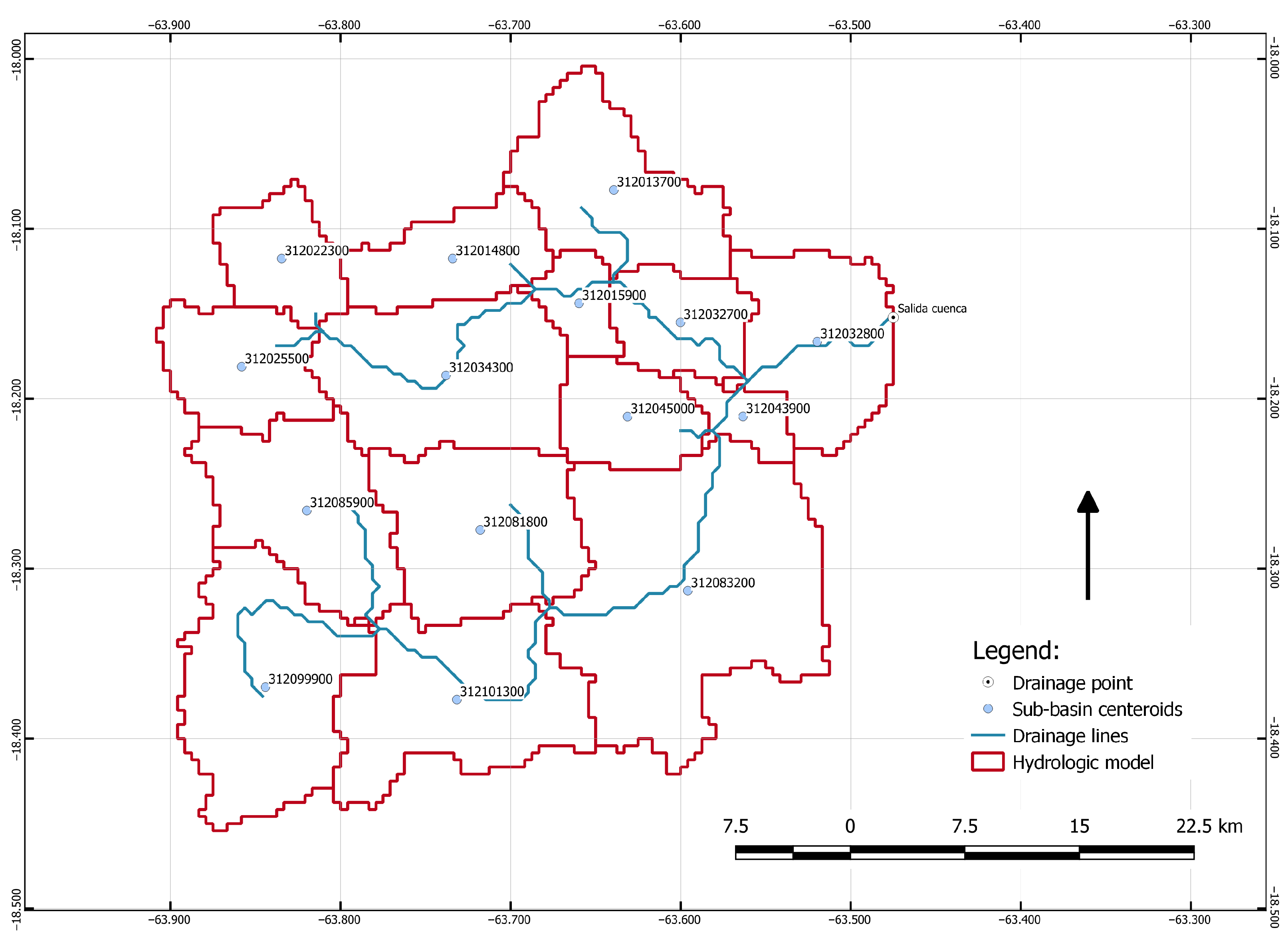
The spatial configuration of the sub-basins to be simulated was carried out based on their respective COMID (the unique identification of each basin within the AHD database; see Figure 7). Following the AHD connectivity flow [33], 15 sub-basins were identified, which compose the Angostura basin as a whole.

COMID 312032800, corresponding to the Angostura basin, was identified, and according to the meteorological information gathered, interpolation to the centroid of the sub-basins was performed through the Climate Data Interpolation Tool (CDIT) inside the HydroBID system.

2.3.3. Calibration and Validation of the Hydrological Model

Calibration was performed in the period from 1 August 1989 to 31 July 1999 and validation from 1 August 1986 to 31 July 1990. Hence, from the 13 hydrological years from the records, it was divided into 70% for calibration and 30% for validation. The calibration process was conducted by trial and error through an iterative process, which implies the manual variation of its parameters. On the other hand, the validation process was simulated using those adjusted parameters in the calibration stage.

2.4. Projections under Climate Change Scenarios

To obtain projections for the specified time periods after the model has been calibrated and validated, future precipitation and temperature values perturbed by both adopted climate change scenarios were used as the input data. Additionally, land use data within the hydrological model, provided by the BID system in its AHD database, were incorporated. This approach enables the estimation of projected streamflow values under climate change scenarios.

2.4.1. Flow Duration Curves

A Flow Duration Curve (FDC) depicts the relationship between the magnitude and frequency of daily, weekly, or monthly (or any other time interval) flows within a specific watershed [34]. It provides an estimation of the percentage of times a certain flow has been equaled or exceeded over a historical period.

An FDC is the complement of the Cumulative Distribution Function (CDF) of daily flow. Each flow value Q corresponds to an exceedance probability p, and an FDC graphically represents $Q_p$, the p-th quantile or percentile of daily flow against the exceedance probability p, where p is defined as:

$$p=1-P\{Q\le q\}$$

(10)

$$p=1-F_Q\left(q\right)$$

(11)

2.4.2. Flow Rate Series

The flow series generated by the HydroBID model, based on average precipitation and temperature projections under 2 climate change scenarios, were compared to the simulated historical runoff for the period 1986–1999. This comparison corresponds to the average annual and monthly runoff of the projected future series in relation to the historical series, as represented by the equation below.

$$\Delta Q_i[\%]=\frac{Q_{project}-Q_{historicsimulated}}{Q_{historicsimulated}}$$

(12)

3. Results

To evaluate the regional climate models (RCMs) obtained by the RegCM4 system through the dynamic downscaling method, six RCMs were generated with the schemes presented in Table 2, in order to obtain two RCMs capable of simulating the climate variables observed during the base period (1981–2010) as closely as possible for the Angostura basin, obtaining the appropriate schema configuration.

In order to test which model better represents the historical values, a Taylor diagram was constructed, as in Figure 8. Subsequently, an evaluation was conducted using the percent bias (PBias) and the Nash–Sutcliffe efficiency coefficient (NSE).

As observed in the Taylor diagram, the models generated by the Sensit02 experiment at a 5 km resolution best represent the ground-measured data. Conversely, the simulated values from the Sensit04 experiment exhibit a high standard deviation and a low correlation coefficient.

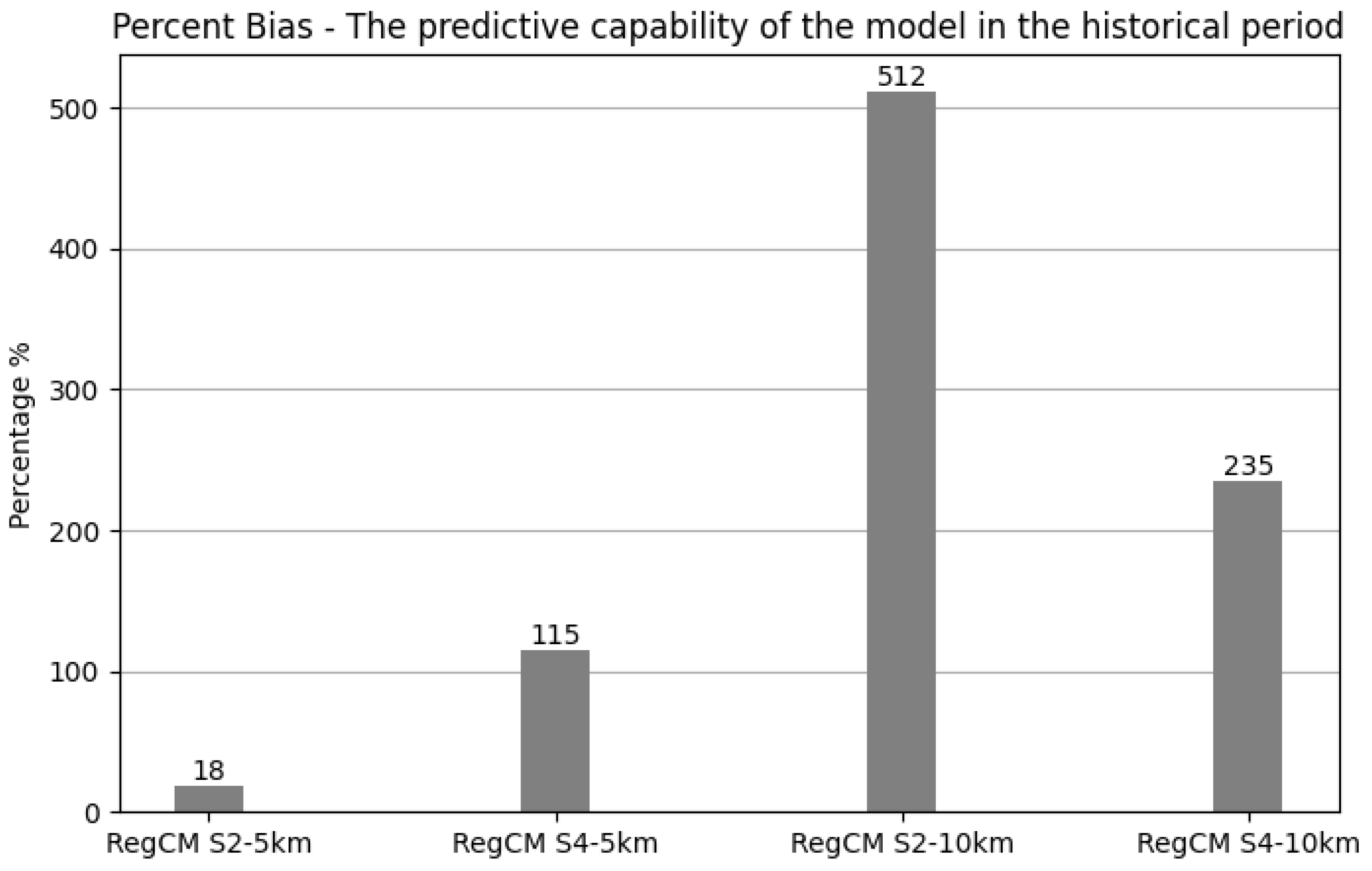
Similarly, the same pattern can be observed with the percentage error in Figure 9, with the Sensit02 experiment at a 5 km resolution being the one that best represents the historical values. Additionally, the Nash–Sutcliffe efficiency (NSE) (see

Table 3. Nash–Sutcliffe efficiency table.

Regional Climate Model	Nash–Sutcliffe
RegCM S2–5 km	0.74
RegCM S2–10 km	−12.41
RegCM S4–5 km	−23.38
RegCM S4–10 km	−26.94

Note: The Sensit02 experiment shows the best efficiency value.

) from this experiment is closest to 1, indicating its capacity to represent the hydroclimatic variables of interest.

From both experiments, the capacity of the Sensit02 experiment to represent the observed climate variables can be seen. This is illustrated by Figure 5 and Figure 6, which show the simulated multiannual average monthly precipitation and temperature (from 2005 to 2015) from the RCM generated by the Sensit02 experiment with a resolution of 5 km related to the data from the observed variables from 1981 to 2010. On the other hand, Figure 6 presents the ability to simulate precipitation over the period from 2005 to 2010, considering as the initial point the RCM from the Sensit04 experiment, to which the statistical downscaling method (SD) by QDM technique will be applied.

Hence, for the purposes of comparing both downscaling methods, the precipitation metrics (see Figure 10) assess the methodology that best represents the observed climate variables and determines which method can be used to make future projections.

The dynamic downscaling (DD) method, the Sensit02 experiment at 5 km resolution to be precise, shows better performance than the statistical downscaling (SD) method based on the precipitation metrics in relation to the observed data. Thus, climate projections were made for the Angostura basin under the Sensit02 experiment schemes for the periods of the 2050s and 2070s under two climate change scenarios defined as RCP 4.5 (as the expected future) and RCP 8.5 (as the pessimistic future) in order to quantify the effects of climate change.

3.1. Hydrologic Modeling Calibration and Validation

The performance indicators are presented in

Table 4. Validation and calibration statistical indicators of the hydrologycal model.

Statistical Indicator	Calibration		Validation
	Daily	Monthly	Daily	Monthly
General volume error (GVE)	−7.50	−7.93	0.65	−0.02
Correlation coefficient (r)	0.84	0.94	0.79	0.93
Modified correlation coefficient (r mod)	0.83	0.63	0.78	0.83
Nash–Sutcliffe efficiency (NSE)	0.68	0.80	0.6	0.86

. According to the Nash–Sutcliffe criterion, the values obtained in the calibration stage are considered “very good” with NSE = 0.68 (daily) and 0.80 (monthly). In the daily validation stage, the fit is “very good” with NSE = 0.6, while at the monthly level, the fit is “excellent” with NSE = 0.86.

The monthly hydrograph of observed and simulated flows, presented in Figure 11 for the calibration and validation stages, shows that the hydrological model is capable of simulating the variability of the flow regime during both flood and low-flow periods. However, there is an underestimation of peak flows for the years between 1990 and 1992.

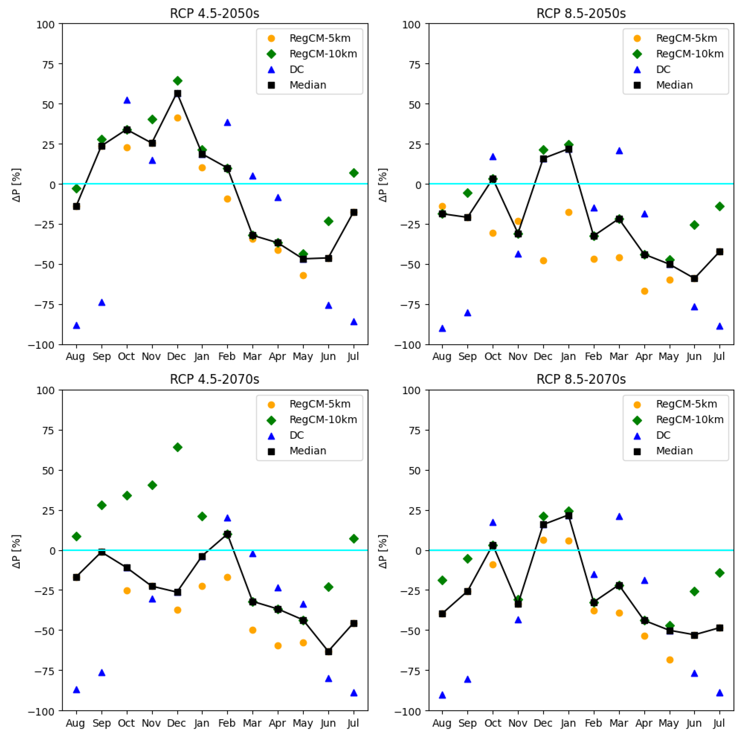
3.2. Rainfall Projection

Figure 12 summarizes the projected changes (relative deltas in %) in precipitation for the Angostura basin. By the 2050s, according to the median, an increase of 9.5% is projected for RCP 4.5 and a decrease of 19.0% for RCP 8.5. On the other hand, a decrease of 11.4% is expected in the 2070s for both scenarios, respectively.

In the near future, the projected changes are not significant. However, future projections show continued decreases in historical cumulative annual average precipitation in the 2070s.

A large variability is observed during the dry months from April to July, as well as a relative change during wet season periods; all other months show an increase in precipitation for the 2050s or, otherwise, slight variations. On the other hand, the period of the 2070s shows a decrease in precipitation at relative deltas in most of the months.

3.3. Precipitation Metrics

The projected precipitation metrics (see Figure 13) were considered to evaluate the future variation in the periods 2050s (a) and 2070s (b).

On the basis of these metrics, an increase is expected for drought days in the coming years. Likewise, an increase for wet days is also expected, which would imply a rise in precipitation intensity for these days as supported by the evidence provided under the third indicator. According to the third indicator, an increase in total precipitation on wet days is expected for the RCP 4.5 scenario. On the other hand, for the RCP 8.5 scenario, as for the other scenario, an increase in drought periods is expected, but a reduction in precipitation during wet spells and total annual precipitation.

3.4. Temperature Projection

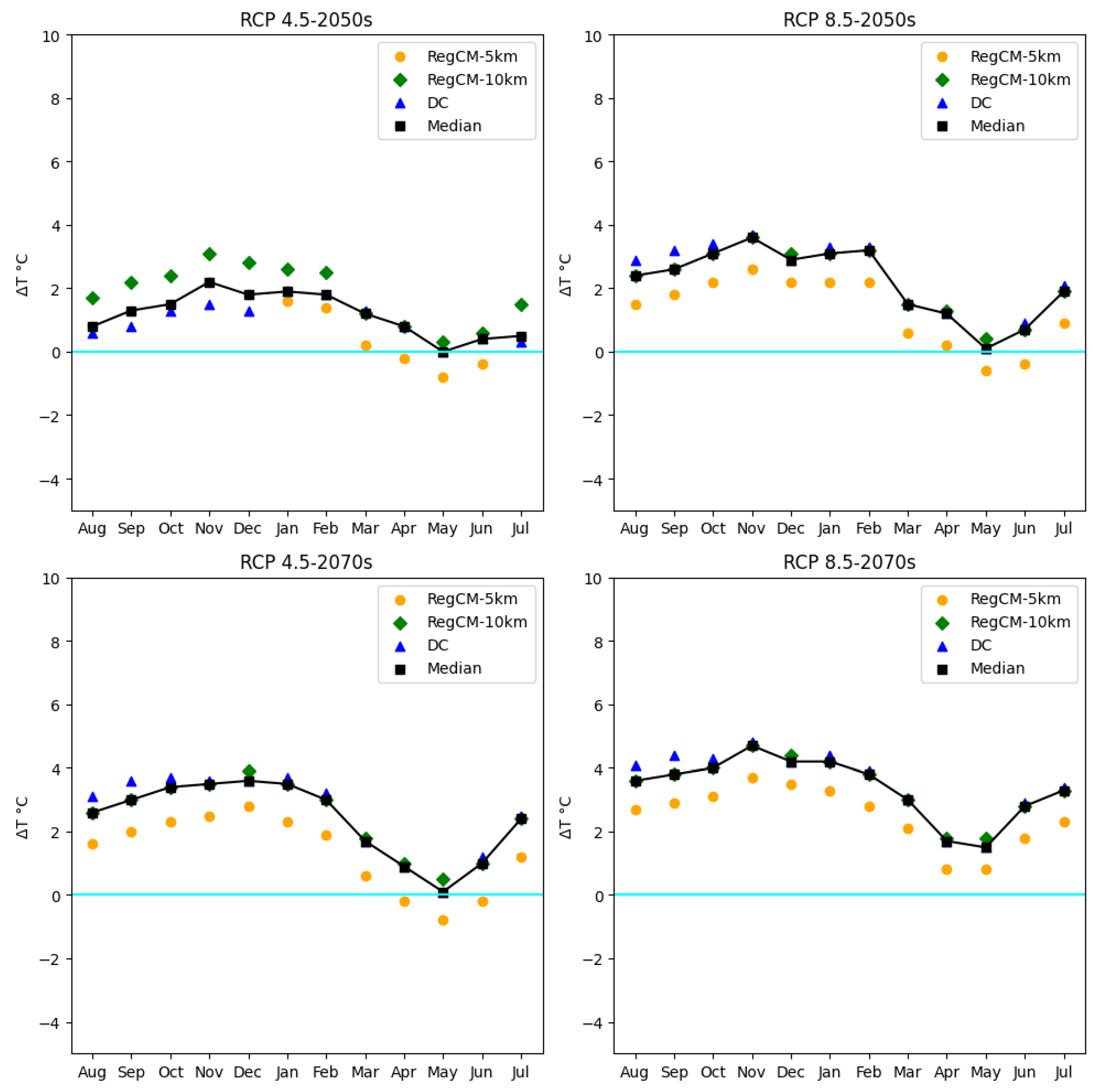
In the near future, projected changes are significant with an increase of approximately 1.3 °C for both scenarios, while an increase in temperature of approximately 3 °C is expected for both future scenarios in the 2070s, as we can see in Figure 14.

To summarize, for both scenarios, a substantial increase will be expected for temperatures, particularly from August to February, according to the relative deltas, while for the cold months, a slight increase is expected, which tends to be low according to the median, whereas the RegCM 5km resolution model shows a slight decrease in 3 of the 4 possible scenarios for the cold months.

The delta-change method has been discarded due to the significant variability it contributed to the precipitation and temperature projection results, in an effort to reduce uncertainty.

3.5. Flow Permanence

Flow permanences display a notorious reduction with respect to the historical period in percentage for all RCP scenarios (see

Table 5. Relative deltas in % permanence curve flows.

RCP 4.5 Scenario
Regional Climate Model (RCM)	Methodology	2050s			2070s
		50%	75%	90%	50%	75%	90%
RegCM-30km	Dynamic Downscaling to 10 km	−15.0	−42.4	−53.0	−46.1	−61.4	−71.2
RegCM-10km	Dynamic Downscaling to 5 km	−49.2	−63.7	−72.0	−83.4	−89.7	−94.3
RCP 8.5 scenario
Regional Climate Model (RCM)	Methodology	2050s			2070s
		50%	75%	90%	50%	75%	90%
RegCM-30km	Dynamic Downscaling to 10 km	−56.9	−66.4	−70.8	−45.5	−61.9	−70.8
RegCM-10km	Dynamic Downscaling to 5 km	−78.4	−85.7	−87.5	−71.9	−85.7	−92.0

), although the most significant decrease was observed among all results obtained from the 5 km resolution RCM under the RCP 8.5 scenario. In order to consider the effect of climate change on a hydraulic project designs, it would be suggested to take the average results from both RCMs.

Therefore, it is inferred that there will be a significant future change in precipitation and temperature under climate change scenarios and, indirectly, in streamflow. According to the medians, water supply would increase during wet months and decrease during dry months in the near (2050s) and distant (2070s) future under RCP 4.5 and would have a similar behavior, but less significant decreasing tendency under RCP 8.5.

4. Discussion

Dynamic downscaling involves a huge computational cost, requiring a cluster to operate and weeks or even months depending on the domain covered by the study area. This is not the case with statistical downscaling, which is simple to apply and does not require specialized machines or a large amount of time to be applied. However, dynamic downscaling simulates more accurate results when it comes to representing the climatic variables of interest, as well as being more versatile due to the large amount of information it generates.

Better resolution in the RCMs leads to a better representation of the variables of interest, especially when it starts from reanalysis data for the development of the RCMs [35], certain aspects of which cannot be adequately captured through statistical downscaling, representing a notable limitation of the SD method. Conversely, dynamic downscaling is heavily influenced by its boundary conditions and demonstrates sensitivity to alterations in multiple parameters within the RegCM4.0 system, necessitating extensive and time-consuming calibration procedures. Therefore, the importance of the dynamic downscaling methodology is emphasized, highlighting an understanding of the inherent limitations of both techniques.

Multiannual mean precipitation projections over the 2050s show a projected increase (according to the median) by 9.5% under the RCP 4.5 scenario and a decrease of 19.0% under the RCP 8.5 scenario. In the near future, projected changes in precipitation vary according to the RCP scenario, whereas future projections for the 2070s show a decrease in both scenarios regarding the historical cumulative annual average precipitation.

The precipitation metrics show an increase in dry spells for both periods and climate change scenarios, an increase in wet spells in the near future (2050s) with a minor increase in wet spells, as well as a decrease in the distant future (2070s), along side the projected increase in total annual precipitation for wet days in the near future and a decrease in the distant future, leading us to conclude that dry spells would be more frequent and the intensity of precipitation on wet days will increase.

Multiannual mean temperature projections show an increase of 1 °C under RCP 4.5 and 1.5 °C under RCP 8.5. On the other hand, by the 2070s, an increase of 2.2 °C and 3.4 °C would be expected for each scenario, respectively. The delta-change results were dropped to prevent changes on average from being affected by the different trend this method displays.

According to the flow projections, water supply would increase during wet months and decrease during dry months in the near (2050s) and distant (2070s) future according to the RCP 4.5 scenario. On the other hand, the RCP 8.5 scenario presents an analogous behavior, but less significant and with a tendency to decrease for most months of the year.

It is well established that, as projections extend further into the future, the level of uncertainty inherent in the results tends to increase. This phenomenon is evident when comparing projections made for two distinct time periods under different climate change (CC) scenarios for fluid flows. Notably, there is a substantial percentage variation between projections for the 2070s compared to those for the 2050s.

5. Conclusions

The RegCM4 system is presented as a versatile tool for evaluating the effects of climate change on water resource potential. Its capability to generate regional climate models (RCMs) at a local-scale resolution sets it apart, eliminating the dependency on pre-existing RCMs, where critical characteristics may be unknown. Nevertheless, its utility is constrained by the significant computational resources it demands and the time investment it necessitates. In response to these challenges, we advocate for a discerning approach to tool selection, tailored to the specific characteristics of the project and desired outcomes. Furthermore, we recommend exploring a broader range of statistical downscaling methods to compile a comprehensive ensemble of results. Such an approach promises to lead us towards more refined outcomes with minimized uncertainty.

The water potential in the Angostura basin would be affected by the new conditions introduced by the effects of climate change. This would manifest as overproduction during wet days and an extended dry season during the dry months. Consequently, it prompts a reconsideration of the design philosophy for water capture infrastructure, which may become obsolete in light of these emerging challenges.

On the other hand, the findings presented in this investigation are constrained by the specific conditions inherent to the Angostura basin, encompassing its geomorphological, spatial, and hydrometeorological characteristics. Hence, it is recommended to duly consider these features when seeking to draw comparisons in future project endeavors.

In addition, this study was deliberately limited in scope to evaluate statistical downscaling methods used for long-term water resources planning studies because of the objectives initially stated.

References

- IPCC. Climate Change 2014: Synthesis Report. Contribution of Working Groups I, II and III to the Fifth Assessment Report of the Intergovernmental Panel on Climate Change; IPCC: Switzerland, Geneva, 2014. [Google Scholar]
- Blöschl, G.; Montanari, A. Climate change impacts-throwing the dice? Hydrol. Process. 2010, 24, 374–381. [Google Scholar] [CrossRef]
- Dai, A. Increasing drought under global warming in observations and models. Nat. Clim. Chang. 2013, 3, 52–58. [Google Scholar] [CrossRef]
- Stehr, A.; Debels, P.; Arumi, J.L.; Alcayaga, H.; Romero, F. Modelación de la respuesta hidrológica al cambio climático: Experiencias de dos cuencas de la zona centro-sur de Chile. Tecnol. Y Cienc. Del Agua 2010, 1, 37–58. [Google Scholar]
- IPCC. Climate Change 2013:The Physical Science Basis.Working Group I Contribution to the Fifth Assessment Report of the Intergovernmental Panel on Climate Change; IPCC: Switzerland, Geneva, 2013; Volume 43, p. 203. [Google Scholar] [CrossRef]
- Gomez-Garcia, M.; Matsumura, A.; Ogawada, D.; Takahashi, K. Time Scale Decomposition of Climate and Correction of Variability Using Synthetic Samples of Stable Distributions. Water Resour. Res. 2019, 55, 3632–3658. [Google Scholar] [CrossRef]
- Gutiérrez, J.M.; Pons, M.R. Modelización numérica del cambio climático: Bases científicas, incertidumbres y proyecciones para la Península Ibérica. Rev. Cuaternario Y Geomorfol. 2006, 20, 15–28. [Google Scholar]
- Xu, Z.; Han, Y.; Yang, Z. Dynamical downscaling of regional climate: A review of methods and limitations. Sci. China Earth Sci. 2019, 62, 365–375. [Google Scholar] [CrossRef]
- Lipa, C.A. Impacto del Cambio Climático en el Aprovechamiento del Potencial hídrico en una Cuenca Piloto en Bolivia. Bachelor’s Thesis, Universidad Mayor de San Simón (UMSS), Cochabamba, Bolivia, 2022. [Google Scholar]
- WMO. Guide to Climatological Practices; World Meteorological Organization: Geneva, Switzerland, 2018; Volume 100, p. 140. [Google Scholar]
- Reboita, M.S.; Fernandez, J.P.R.; Llopart, M.P.; Rocha, R.P.D.; Pampuch, L.A.; Cruz, F.T. Assessment of RegCM4.3 over the CORDEX South America domain: Sensitivity analysis for physical parameterization schemes. Clim. Res. 2014, 60, 215–234. [Google Scholar] [CrossRef]
- Giorgi, F.; Gutowski, W.J. Regional Dynamical Downscaling and the CORDEX Initiative. Annu. Rev. Environ. Resour. 2015, 40, 467–490. [Google Scholar] [CrossRef]
- Martínez, P.; Patiño, C. Efectos del cambio climático en la disponibilidad de agua en México. Tecnol. Y Cienc. Del Agua 2012, 3, 5–20. [Google Scholar]
- Huang, J.; Zhang, J.; Zhang, Z.; Xu, C.Y.; Wang, B.; Yao, J. Estimation of future precipitation change in the Yangtze River basin by using statistical downscaling method. Stoch. Environ. Res. Risk Assess. 2011, 25, 781–792. [Google Scholar] [CrossRef]
- Cannon, A.J.; Sobie, S.R.; Murdock, T.Q. Bias correction of GCM precipitation by quantile mapping: How well do methods preserve changes in quantiles and extremes? J. Clim. 2015, 28, 6938–6959. [Google Scholar] [CrossRef]
- Campozano, L.; Tenelanda, D.; Sanchez, E.; Samaniego, E.; Feyen, J. Comparison of Statistical Downscaling Methods for Monthly Total Precipitation: Case Study for the Paute River Basin in Southern Ecuador. Adv. Meteorol. 2016, 2016, 6526341. [Google Scholar] [CrossRef]
- Osma, V.C.; Romá, J.E.C.; Martín, M.A.P. Modelling regional impacts of climate change on water resources: The Júcar basin, Spain. Hydrol. Sci. J. 2013, 60, 30–49. [Google Scholar] [CrossRef]
- FAO. The Digital Soil Map of the World; FAO: Rome, Italy, 2003. [Google Scholar]
- Ekström, M.; Grose, M.R.; Whetton, P.H. An appraisal of downscaling methods used in climate change research. Wiley Interdiscip. Rev. Clim. Chang. 2015, 6, 301–319. [Google Scholar] [CrossRef]
- Giorgi, F.; Coppola, E.; Solmon, F.; Mariotti, L.; Sylla, M.B.; Bi, X.; Elguindi, N.; Diro, G.T.; Nair, V.; Giuliani, G.; et al. RegCM4: Model description and preliminary tests over multiple CORDEX domains. Clim. Res. 2012, 52, 7–29. [Google Scholar] [CrossRef]
- Dee, D.P.; Uppala, S.M.; Simmons, A.J.; Berrisford, P.; Poli, P.; Kobayashi, S.; Andrae, U.; Balmaseda, M.A.; Balsamo, G.; Bauer, P.; et al. The ERA-Interim reanalysis: Configuration and performance of the data assimilation system. Q. J. R. Meteorol. Soc. 2011, 137, 553–597. [Google Scholar] [CrossRef]
- Sheridan, S.C.; Lee, C.C.; Smith, E.T. A Comparison Between Station Observations and Reanalysis Data in the Identification of Extreme Temperature Events. Geophys. Res. Lett. 2020, 47, e2020GL088120. [Google Scholar] [CrossRef]
- Hakala, K.; Addor, N.; Seibert, J. Hydrological modeling to evaluate climate model simulations and their bias correction. J. Hydrometeorol. 2018, 19, 1321–1337. [Google Scholar] [CrossRef]
- Willems, P.; Vrac, M. Statistical precipitation downscaling for small-scale hydrological impact investigations of climate change. J. Hydrol. 2011, 402, 193–205. [Google Scholar] [CrossRef]
- Fiseha, B.M.; Melesse, A.M.; Romano, E.; Volpi, E.; Fiori, A. Statistical Downscaling of Precipitation and Temperature for the Upper Tiber Basin in Central Italy. Int. J. Water Sci. 2012, 1, 1. [Google Scholar] [CrossRef][Green Version]
- Boé, J.; Terray, L.; Habets, F.; Martin, E. Statistical and dynamical downscaling of the Seine basin climate for hydro-meteorological studies. Int. J. Climatol. 2007, 27, 1643–1655. [Google Scholar] [CrossRef]
- Maraun, D.; Wetterhall, F.; Ireson, A.M.; Chandler, R.E.; Kendon, E.J.; Widmann, M.; Brienen, S.; Rust, H.W.; Sauter, T.; Themel, M.; et al. Precipitation downscaling under climate change: Recent developments to bridge the gap between dynamical models and the end user. Rev. Geophys. 2010, 48, RG3003. [Google Scholar] [CrossRef]
- Paz, S.M.; Willems, P. Uncovering the strengths and weaknesses of an ensemble of quantile mapping methods for downscaling precipitation change in Southern Africa. J. Hydrol. Reg. Stud. 2022, 41, 101104. [Google Scholar] [CrossRef]
- Teutschbein, C.; Seibert, J. Bias correction of regional climate model simulations for hydrological climate-change impact studies: Review and evaluation of different methods. J. Hydrol. 2012, 456–457, 12–29. [Google Scholar] [CrossRef]
- Gutmann, E.; Pruitt, T.; Clark, M.P.; Brekke, L.; Arnold, J.R.; Raff, D.A.; Rasmussen, R.M. An intercomparison of statistical downscaling methods used for water resource assessments in the United States. Water Resour. Res. 2014, 50, 7167–7186. [Google Scholar] [CrossRef]
- Moreda, F.; Miralles-Wilhelm, F.; Castillo, R.M. Hydro-BID: Un Sistema Integrado para la Simulación de Impactos del Cambio Climático sobre los Recursos Hídricos. Parte 2 Banco Interamericano de Desarrollo. Available online: https://publications.iadb.org/es/publicacion/16910/hydro-bid-un-sistema-integrado-para-la-simulacion-de-impactos-del-cambio (accessed on 10 May 2022).
- Dingman, S.L. Physical Hydrology, 3rd ed.; Waveland Press, Inc.: Long Grove, IL, USA, 2015; p. 643. [Google Scholar]
- Rineer, J.; Bruhn, M.; Miralles, F.; Raúl, W.; Castillo, M. Base de Datos de Hidrología Analítica para América Latina y el Caribe. Parte 1. Available online: https://publications.iadb.org/es/base-de-datos-de-hidrologia-analitica-para-america-latina-y-el-caribe (accessed on 10 May 2022).
- Vogel, R.M.; Fennessey, N.M. Flow-Duration Curves. I: New Interpretation and Confidence Intervals. J. Water Resour. Plan. Manag. 1994, 120, 485–504. [Google Scholar] [CrossRef]
- Eini, M.R.; Javadi, S.; Delavar, M.; Monteiro, J.A.; Darand, M. High accuracy of precipitation reanalyses resulted in good river discharge simulations in a semi-arid basin. Ecol. Eng. 2019, 131, 107–119. [Google Scholar] [CrossRef]
Figure 1.
Flowchart resume of methodology through the different phases of the paper.
Figure 2.
Location of the study area in the department of Santa Cruz-Bolivia, a country of South America.
Figure 3.
Representative total annual precipitation, period of 1981/1982 to 2009/2010.
Figure 4.
Extraction methods’ RCM precipitation series, period of 2005–2015 with 5 km resolution. (a) The first method consists of extracting the data from the grid closest to the basin’s 100 centroid coordinates; (b) the second method involves taking the average of all grids overlapping across the basin area and (c) obtaining the average of the grids closest to the coordinates of each station within the basin.
Figure 5.
Extraction methods’ RCM temperature series, period of 2005–2015 with 5 km resolution. (a) The first method consists of extracting the data from the grid closest to the basin’s 100 centroid coordinates; (b) the second method involves taking the average of all grids overlapping across the basin area and (c) obtaining the average of the grids closest to the coordinates of each station within the basin.
Figure 6.
Rainfall time series by SD through the QDM method. (a) Sensitive02 experiment with a 10 km resolution; (b) Sensitive04 with a 10 km resolution.
Figure 7.
Delimitation of sub-basins in the study area according to their COMIDs.
Figure 8.
Taylor diagram to assess the simulation capability of the model. (a) The first method consists of extracting the data from the grid closest to the basin’s 100 centroid coordinates; (b) the second method involves taking the average of all grids overlapping across the basin area and (c) obtaining the average of the grids closest to the coordinates of each station within the basin.
Figure 9.
Predictive capability of the model in the historical period through the percent bias (PBias). A comparison is made of the percent bias of 4 RCM models generated by the RegCM4.0 system from both experiments with resolutions of 5 km and 10 km.
Figure 10.
DD vs. SD precipitation climate metrics.
Figure 11.
Time series of observed and modeled monthly flows.
Figure 12.
Projected changes in multiannual average monthly precipitation.
Figure 13.
Changes in precipitation metrics over the future period for 2 climate change scenarios. Maximum length of dry spell (consecutive dry days < 1 mm, CDD), maximum length of wet spell (consecutive wet days ≥1 mm, CWD), and annual total precipitation for wet days (PRCPTOT).
Figure 14.
Projected changes in multiannual average monthly temperature.