Ensemble Forecasts of Extreme Flood Events with Weather Forecasts, Land Surface Modeling and Deep Learning

Abstract

Integrating numerical weather forecasts that provide ensemble precipitation forecasts, land surface hydrological modeling that resolves surface and subsurface hydrological processes, and artificial intelligence techniques that correct the forecast bias, known as the “meteo-hydro-AI” approach, has emerged as a popular flood forecast method. However, its performance during extreme flood events across different interval basins has received less attention. Here, we evaluated the meteo-hydro-AI approach for forecasting extreme flood events from headwater to downstream sub-basins in the Luo River basin during 2010–2017, with forecast lead times up to 7 days. The proposed meteo-hydro approach based on ECMWF weather forecasts and the Conjunctive Surface-Subsurface Process version 2 land surface model with a spatial resolution of 1 km captured the flood hydrographs quite well. Compared with the ensemble streamflow prediction (ESP) approach based on initial conditions, the meteo-hydro approach increased the Nash-Sutcliffe efficiency of streamflow forecasts at the three outlet stations by 0.27–0.82, decreased the root-mean-squared-error by 22–49%, and performed better in reliability and discrimination. The meteo-hydro-AI approach showed marginal improvement, which suggested further evaluations with larger samples of extreme flood events should be carried out. This study demonstrated the potential of the integrated meteo-hydro-AI approach for ensemble forecasting of extreme flood events.

1. Introduction

Flooding is one of the most devastating natural disasters that causes serious economic losses and casualties [1]. In particular, flash floods due to extreme precipitation in mountainous basins are very difficult to forecast, which challenges current early warning systems [2]. With the increase in global temperature and extreme precipitation [3], as well as the nonstationarity of streamflow [4,5,6], flood forecasting has been an important non-engineering measure for disaster prevention and climate change adaptation.

Flood forecasting has experienced rapid development since the last century. The currently popular methods include empirical forecasting [7], hydrological modeling [8,9], and data-driven modeling [10,11]. Empirical forecasting methods often have low accuracy because the parameters are difficult to quantify [12]. Data-driven methods necessitate a substantial amount of data training to obtain reliable results [13], and the performance from training to testing is usually unstable [14]. These two methods cannot explain the complex land surface hydrological processes in the watershed. Compared with lumped hydrological models, the distributed hydrological models are more complex in structure and can account for the spatial heterogeneity of hydrological processes [15,16]. At present, incorporating small-scale physical hydrological processes into high-resolution land surface hydrological models that resolve both fine-scale topography and the rainfall-runoff relationship is urgently needed in flood simulation and forecasting [6,17,18].

When the land surface hydrological model is used to forecast floods, it is affected by various sources of uncertainty, such as initial hydrological conditions, meteorological forcing inputs, model structure, and parameters [9,19]. The lack of uncertainty information in single-value forecasting hardly represents the full possibility of future streamflow, which will affect the accuracy of flood forecasting and limit its application. In order to obtain better forecast results, the ensemble method is applied to hydrological forecasts. The ensemble streamflow prediction (ESP) method considers uncertainty by generating streamflow forecasts using historical meteorological forcing and is still widely used nowadays [20]. For example, Wood and Lettenmaier [21] used the ESP method to predict streamflow with a 5-month lead time in northern California during the drought-flood transition period. Sabzipour et al. [22] improved ESP forecasting potential by using a genetic algorithm to screen historical meteorological forcing datasets. In recent years, the rapid development of numerical weather forecasts has led to significant improvement in precipitation forecasting [23,24,25,26], which can even provide a skillful forecast of heavy rainfall several days in advance [27,28]. Therefore, many studies have begun to use ensemble meteorological forecasting from numerical weather forecasts to obtain ensemble flood forecasting [29,30,31,32].

Even though the meteo-hydro forecast approach has been widely applied in short-term and long-term streamflow forecasts [29,33], there remains significant uncertainty. On one hand, hydrological processes are very complex and affected by multiple factors, including the interaction of meteorological, environmental, and human activities. On the other hand, there are scale-mismatch issues in the modeling. Therefore, it is difficult to cover all physical processes in the land surface hydrological models [34,35], and post-processing of the hydrological forecasts is often applied to eliminate system bias for both deterministic and probabilistic forecasts [8,36].

Recent studies have shown that machine learning or deep learning methods can identify hidden rules and trends from datasets without understanding the physical mechanisms of hydrological processes and have great potential to overcome the limitations of hydrological models and reduce model errors [11,37,38,39,40]. Yang et al. [41] combined physical hydrological model simulations with machine learning to improve streamflow simulation in northern Thailand. Konapala et al. [42] established a hybrid model combining machine learning and hydrological modeling, which could improve the streamflow simulation results of different basins in the United States compared with the hydrological model. Cho and Kim [43] used the long short-term memory (LSTM) algorithm to predict the residuals of the output streamflow simulation of the WRF-Hydro model, which significantly improved the Nash-Sutcliffe efficiency (NSE) of daily streamflow. However, most studies focused on the simulations of long-term trends or monthly/daily streamflow, while the potential for improvement of extreme flood forecasts at an hourly timescale remains to be explored, especially for those integrated with a numerical weather forecast model.

In this study, we combined LSTM with the meteo-hydro forecast method to predict the four largest flood events in the sub-basins of the Luo River from 2010 to 2017. We used the meteorological hindcast datasets from the European Centre for Medium-Range Weather Forecasts (ECMWF) in the International Grand Global Ensemble (TIGGE) project to drive the high-resolution land surface hydrological model, named “CSSPv2” (Conjunctive Surface-Subsurface Process version 2) [6], and used the LSTM method to correct the meteo-hydro ensemble flood forecasting. We strived to (1) verify the ability of CSSPv2 to simulate extreme flood events; (2) investigate the impact of the meteorological forecasts (i.e., ECMWF) on extreme flood forecasts; and (3) explore the added value of the deep learning method.

2. Materials and Methods

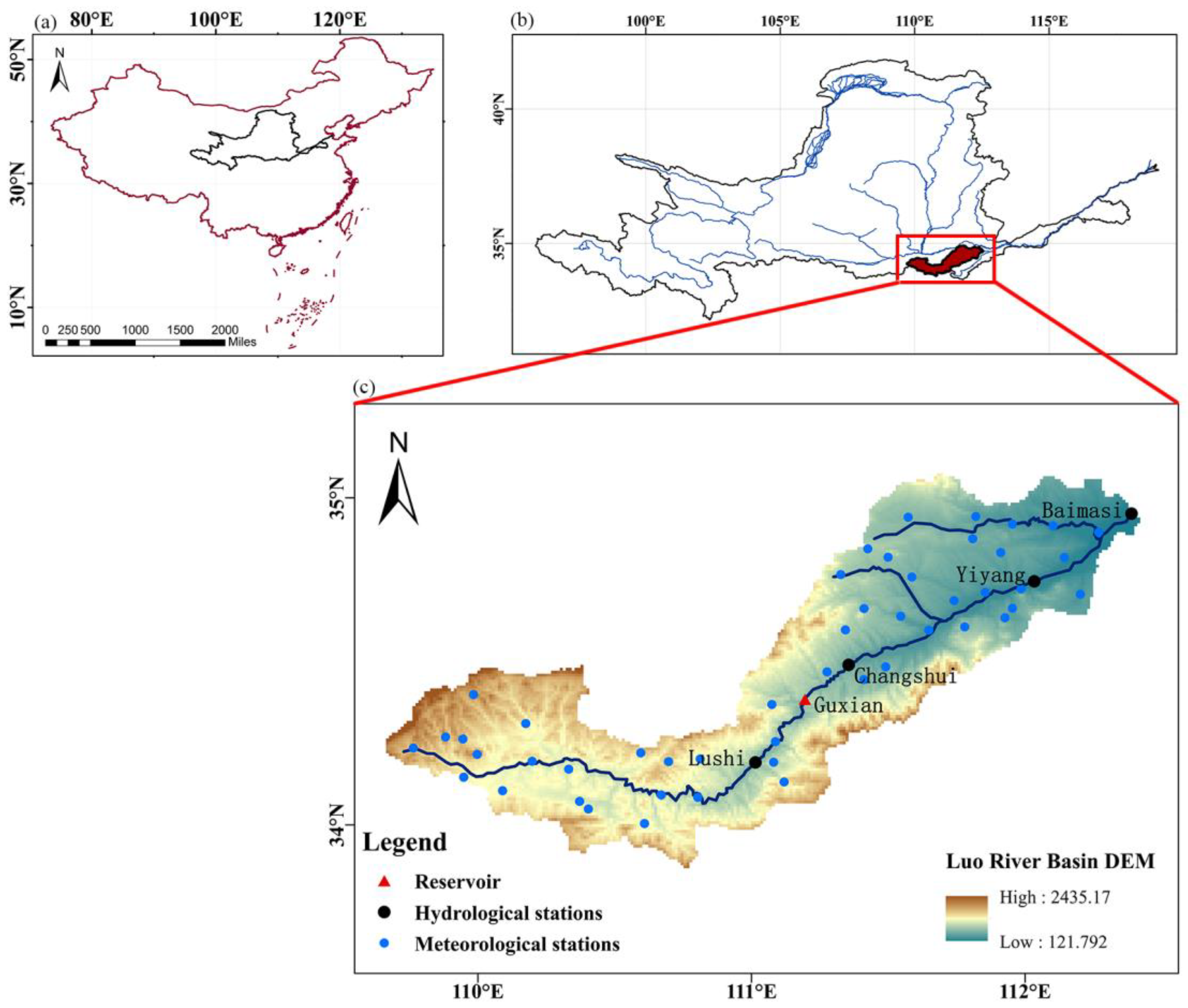
2.1. Study Area and Data

The Luo River is a branch of the Yiluo River, a main tributary of the middle reach of the Yellow River in China (Figure 1a,b). It flows through Shaanxi and Henan Provinces, with a total length of 447 km. The basin area above the Baimasi station (Figure 1c) is 11,891 km². The Luo River is one of the tributaries with sufficient water resources in the Yellow River basin. There are four hydrological stations in the basin, i.e., Lushi, Changshui, Yiyang and Baimasi (Figure 1c). Because there is the Guxian Reservoir in the interval basin between Lushi and Changshui, this study only focused on the other three interval basins: from headwater to Lushi, from Changshui to Yiyang, and from Yiyang to Baimasi. Except for the Lushi station, the observed upstream outflow was input into the land surface hydrological model for the simulations and forecasts of the downstream floods.

The meteorological forcing data that drive the land surface hydrological model for flood forecasting include precipitation, temperature, pressure, specific humidity, wind speed, and surface downward longwave and shortwave radiation. The hourly precipitation data from 51 hydrological stations were interpolated to a 1 km grid by the inverse quadratic distance weighting method, and other meteorological forcing data were interpolated from the 6-km China Meteorological Forcing Dataset (CMFD) by the bilinear interpolation method [44].

TIGGE is a key component of the THORPEX project started in October 2006, which includes ensemble forecast data from 10 numerical weather prediction centers around the world, including the ECMWF. This study used 7-day meteorological reforecast data from the ECMWF model with 51 ensemble members, which started at 00Z on the beginning day of the extreme flood event. The bilinear interpolation method was used to interpolate precipitation and temperature reforecasts from 0.5-degree to 1-km resolution.

The meteorological forcing datasets used by ESP were resampled from historical observational data. For each extreme flood event, the 7-day meteorological forcing (including precipitation, temperature, etc.) for the target calendar week, and one week before and one week after the calendar week during 2006–2020 (excluding the target year) were selected, resulting in 14 (years) × 3 (weeks) = 42 samples. Then, half of the samples (i.e., 21) with a larger 7-day precipitation amount were selected as the ensemble members of ESP.

The observed hourly streamflow data at Lushi, Yiyang, and Baimasi stations (Figure 1c) during June–October of 2010–2017 were obtained from the local authority. They were used for model calibration and verification. The extreme flood events were identified by ranking flood peaks according to the time series of hourly streamflow. The highest four peaks were selected for each hydrological station. The starting date of the extreme flood events was the day with the lowest hourly streamflow as traced back from the peak day, and the end date was the day with hourly streamflow lower than the 90th percentile. For the meteo-hydro reforecast, only the first 7 days were selected for verification. If the flood event was less than 7 days, the preceding day would be used as the beginning day of the flood event.

2.2. Methods

Figure 2 is a flowchart of the meteo-hydro-AI reforecasts carried out in this study. We generated ESP streamflow forecasts by using the CSSPv2 model (see Section 2.2.1 for details) driven by datasets resampled from historical meteorological data. Alternatively, the ESP meteorological forcings were replaced with ECMWF meteorological reforecasts. For the hydrological stations at the middle and lower reaches of the Luo River, observed upstream streamflow was used as input for the river routing model in CSSPv2. After meteo-hydro forecasts, the results were corrected by the LSTM deep learning model (see Section 2.2.2 for details). The evaluation metrics (see Section 2.2.3 for details) used in this paper include deterministic and probabilistic methods.

2.2.1. CSSPv2 Land Surface Hydrological Model

The land surface hydrological model used in this study is the CSSPv2 model [6], which is based on the Common Land Model [45] while providing a better representation of land surface hydrology. CSSPv2 has a volume-averaged soil water transport module that considers the influence of sub-grid topographic variation [46], a groundwater module that interacts with soil water movement [47], a runoff generation scheme based on the variable infiltration capacity (VIC) scheme [15], and a routing model based on a linear transport scheme. The routing is calculated as:

$$F_{out}=\frac{v}{d}S$$

(1)

$$v=\max \left(vmin,k{\beta }^{0.5}\right)$$

(2)

where $F_{out}$ is the water flux leaving the grid, v is the effective water flow velocity, d is the distance between this grid and the downstream grid, S is the volume of river water stored within the grid, β is the grid cell mean topographic slope from a high-resolution elevation database, $vmin$ and k are the routing parameters that need to be calibrated. In addition, we also need to calibrate three VIC parameters for runoff generation, i.e., $D_s$, $D_{s,\max }$, and b factor (

Table 1. Runoff generation and river routing parameters of CSSPv2 over each interval sub-basin.

Parameters	Description	Lushi	Yiyang	Baimasi
$b$	Exponent of variable infiltration capacity curve	1.40	0.04	5.30
$D_s$	Fraction of maximum base flow	0.011	0.010	0.012
$D_{s,max}$	Maximum velocity of base flow (m/s)	5.13 × 10−3	3.00 × 10−7	3.70 × 10−5
$vmin$	Minimum grid effective flow velocity (m/s)	0.74	3.00	0.80
$k$	Grid effective flow velocity slope parameters	1.80	8.00	1.60

) for three interval catchments separately. $D_s$ is the fraction of maximum base flow. $D_{s,\max }$ is the maximum velocity of base flow (m/s). b is the exponent of the variable infiltration capacity curve. We first determined the range of parameter values [48]. For the Lushi basin, the parameters’ values were modified directly by manual adjustment. For Changshui-Yiyang and Yiyang-Baimasi interval catchments, the hourly streamflow of the upstream gauge (i.e., Changshui, Yiyang) at the corresponding grid point was added as the upstream input, then the parameters were calibrated to increase the NSE value. More than 200 sets of parameters were tested in each interval basin. The parameters are shown in Table 1.

2.2.2. LSTM Deep Learning Model

The LSTM is a recurrent neural network model with a unique structure [49]. It learns the long-term nonlinear relationship between variables through the combination of forgetting gate, input gate, and output gate. Since the LSTM model has the ability of selective memory and can better deal with noise in long time series, it is suitable for the study of time series of hydrological variables [50,51,52].

In this study, we set up two sets of LSTM experiments. The LSTM-CV was a cross-validation procedure, and the model used to correct each flood event was obtained based on the data from the other three floods. The LSTM-ALL trained all four flood events together without cross validation and was considered the upper limit of the ability of the LSTM model in correcting extreme flood forecasts. The model was established for each ensemble member, and the input data were hourly streamflow observation data and forecast data. During the training, the streamflow observation data of the target hour, and five hours of forecast streamflow data before the target hour were used to calibrate the LSTM model, with a sample size of 168 − 5 = 163 for each flood event. Therefore, there were 163 × 3 samples for LSTM-CV, and 163 × 4 samples for LSTM-ALL. In the correction, the streamflow at the target hour was corrected by using the LSTM model with streamflow forecasts in the previous 5 h. In this study, the LSTM model with a forgetting gate was used, and the Adam optimizer was selected, which was an effective way to optimize the LSTM model [53]. According to existing research and model tests [54], the batch size and epoch were set at 450 and 300, respectively.

2.2.3. Evaluation Metrics

In this study, the deterministic evaluation indicators include NSE, root mean square error (RMSE), relative absolute bias (rBIAS), and correlation coefficients (CCR). The metrics are computed as follows:

$$NSE=1-\frac{\sum _{i=1}^n{\left(Q_{obs,i}-Q_{sim,i}\right)}^2}{\sum _{i=1}^n{\left(Q_{obs,i}-\overline{Q_{obs}}\right)}^2}$$

(3)

$$RMSE=\frac{\sum _{i=1}^n{\left(Q_{obs,i}-Q_{sim,i}\right)}^2}{n}$$

(4)

$$rBIAS=\frac{\sum _{i=1}^n{|Q}_{obs,i}-Q_{sim,i}|}{\sum _{i=1}^n{Q}_{obs,i}}\times 100\%$$

(5)

$$CCR=\frac{\sum _{i=1}^n{(Q}_{obs,i}-\overline{Q_{obs}}){(Q}_{sim,i}-\overline{Q_{sim}})}{\sqrt{\sum _{i=1}^n{\left(Q_{obs,i}-\overline{Q_{obs}}\right)}^2}\sqrt{\sum _{i=1}^n{\left(Q_{sim,i}-\overline{Q_{sim}}\right)}^2}}$$

(6)

where $Q_{obs}$ is observed streamflow, and $Q_{sim}$ is simulated or predicted streamflow.

The probabilistic evaluation procedures include the reliability diagram and relative operating characteristic (ROC) diagram [55]. The reliability diagram has two elements, which are conditional distributions of the observation given each of the redistributed probability forecast range, $p\left(o_j\right|y_i)$, and the refinement distribution $p\left(y_i\right)$. The ROC diagram is a discrimination-based graphical forecast verification display. In addition, the continuous ranked probability skill score (CRPSS) [55] was also used for assessing the accuracy of probabilistic forecasts of extreme floods.

3. Results

3.1. Calibration of CSSPv2 Land Surface Hydrological Model

In the Luo River basin, we selected the four largest floods during June–October from 2010 to 2017 for each of the three hydrological stations (i.e., Lushi, Yiyang, and Baimasi) to calibrate the CSSPv2 land surface hydrological model. Figure 3 shows the calibration results. The calibrated CSSPv2 model can capture the flood peaks and the entire processes. The maximum flood peak flows of Lushi, Yiyang and Baimasi stations were 1660 m³/s, 1835 m³/s, and 2270 m³/s respectively. The model simulations of the maximum flood peaks were still biased, with underestimations for several flood events. The NSE values of hourly streamflow at Lushi, Yiyang, and Baimasi stations were 0.54, 0.55, and 0.66 respectively, and the CCR values were greater than 0.8 (

Table 2. Evaluation of hourly streamflow simulations by the calibrated CSSPv2 land surface hydrological model for each interval sub-basin.

Title 1	NSE	RMSE	rBIAS	CCR
Lushi	0.54	278.39	36.71%	0.81
Yiyang	0.55	184.81	24.15%	0.88
Baimasi	0.66	250.17	27.06%	0.89

). In general, the CSSPv2 model well simulated the extreme floods of the three basins.

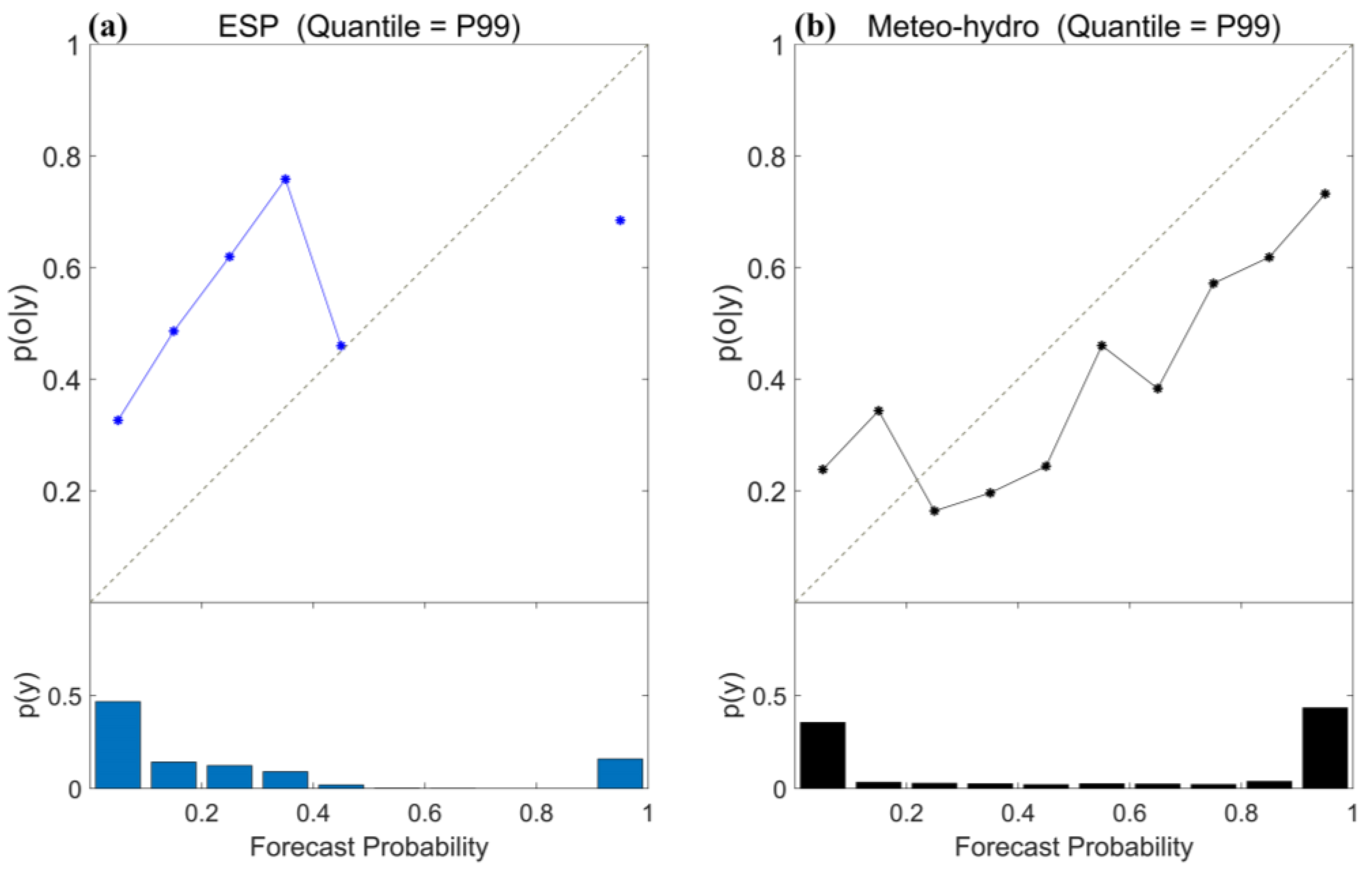
3.2. Evaluation of Ensemble Precipitation Forecasts from ECMWF

Before assessing the meteo-hydro ensemble forecasts, we first evaluated the ECMWF precipitation reforecasts. Figure 4 shows the evaluation of ECMWF precipitation reforecasts during the 7-day flood periods at the interval sub-basins of Lushi, Yiyang, and Baimasi. Most of the forecast results showed larger errors and uncertainty ranges at the peak of precipitation. The predicted extreme precipitation was basically consistent with observations at the Lushi sub-basins, and the observed precipitation was always within the range of ensemble precipitation forecasts (Figure 4a–d). The peak values of precipitation in the Yiyang and Baimasi sub-basins were mostly lagging behind, and the ensemble mean values of the predicted precipitation are significantly lower than the observed precipitation (Figure 4e–l). In addition, the ECMWF model missed the first peak values of precipitation in the two sub-basins on 14 September 2014 (Figure 4h,l). The average NSE and CCR of Lushi precipitation ensemble forecasts were 0.73 and 0.89, which was in good agreement with the observed precipitation. Due to the lag and deviation of precipitation forecasts, the NSE for Yiyang and Baimasi were 0.24 and 0.12, and the CCR were 0.47 and 0.42, which has certain forecast skills.

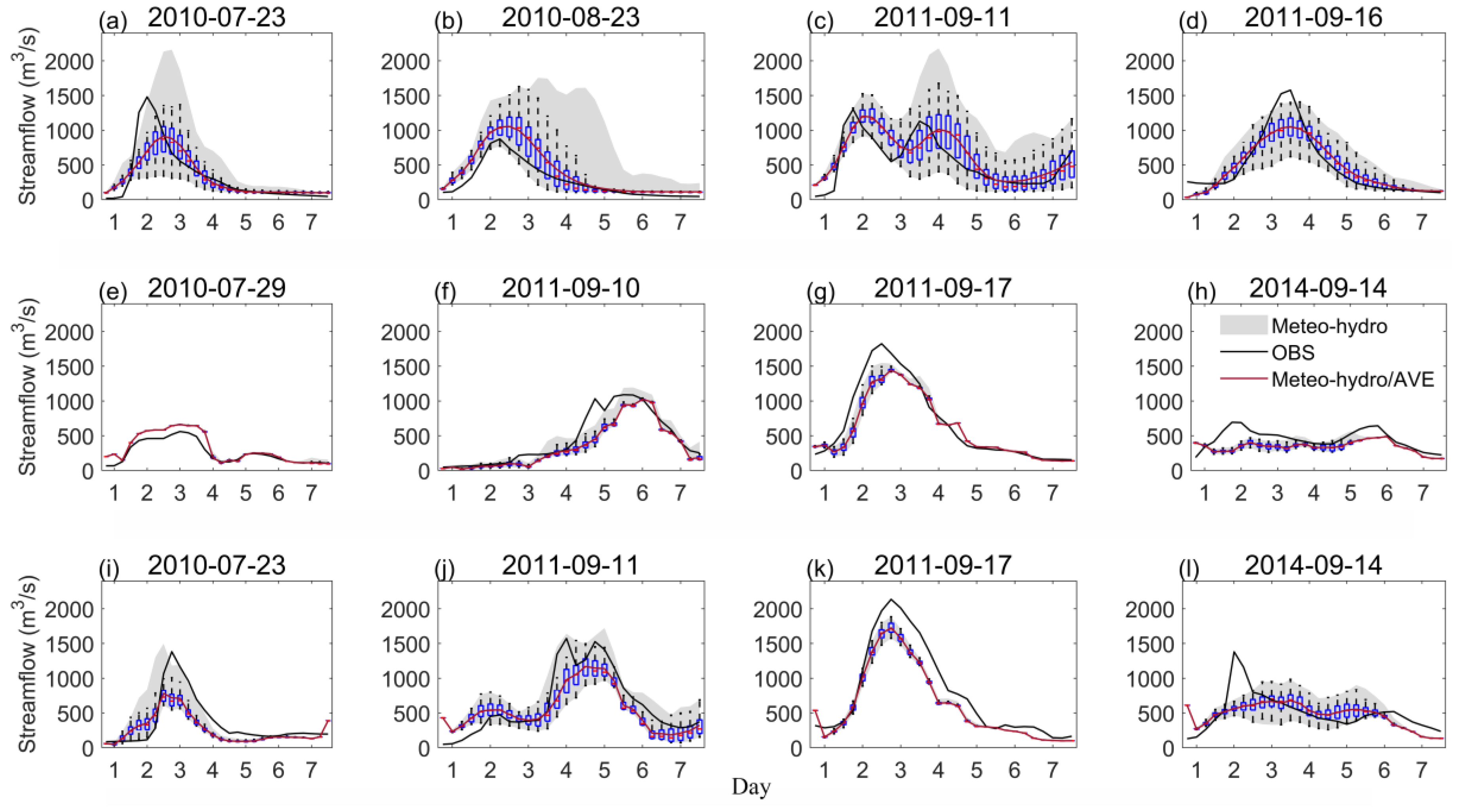
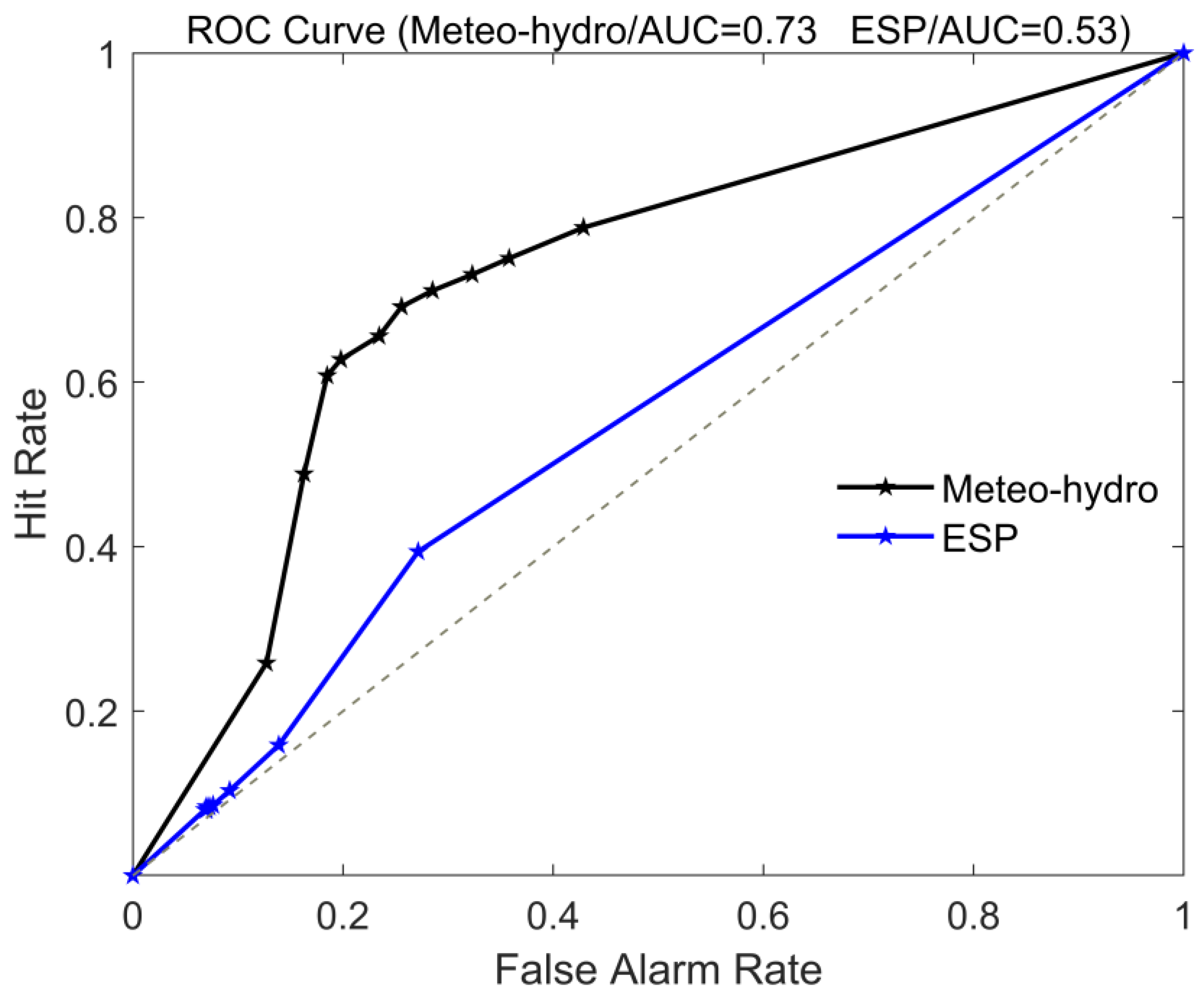
3.3. Evaluation of Meteo-Hydro Ensemble Flood Forecasts from ECMWF/CSSPv2

The results of this part are from CSSPv2 land surface hydrological forecasts driven by the ECMWF meteorological ensemble forecasts. Figure 5 shows the 7-day flood forecasts as compared with the observed hourly streamflow for four of the largest floods at Lushi, Yiyang, and Baimasi stations. The meteo-hydro ensemble forecasts can predict the evolution of floods at the three stations and can roughly capture the flood peaks, although with overestimations or underestimations. For the first flood peaks at Yiyang and Baimasi stations on 14 September 2014, the meteo-hydro forecasts missed them (Figure 5h,l) because the precipitation peaks are not captured by the ECMWF model (Figure 4h,l).

Comparing the ECMWF/CSSPv2-based meteo-hydro ensemble flood forecasts with the ESP/CSSPv2-based forecasts, the former shows obvious advantages. As shown in Figure 6, the NSE values of ECMWF/CSSPv2 streamflow forecasts are higher than those of ESP/CSSPv2 by 0.82, 0.27, and 0.37 for the three hydrological stations, respectively. Moreover, the meteo-hydro forecast reduces RMSE from ESP by 49%, 22%, and 24%. From ESP/CSSPv2 to ECMWF/CSSPv2 forecasts, the rBIAS of the three stations decreases by 14% on average, and the CCR increases by 72%. The CRPSS (=1-CRPS_ECMWF/CSSPv2/CRPS_ESP/CSSPv2) values are 0.54, 0.19, and 0.25 for the three hydrological stations, which suggests that the meteo-hydro forecast approach has higher probabilistic forecast skill than the ESP approach.

The reliability diagram (Figure 7) is a full graphical representation of the joint distribution of the forecasts and observations. When the curve is distributed along the diagonal (1:1) line, the forecast result is considered reliable. Figure 7 shows the reliability of ESP and meteo-hydro ensemble forecasts. The meteo-hydro ensemble forecast had an under-dispersion error, where the curve was above the diagonal line when the forecast probability is low, and below the diagonal line when the forecast probability is high (Figure 7b). That meant the forecast results were underestimated for the low flows and overestimated for the high flows, which suggested the forecast results were overconfident. However, compared to the ESP, the meteo-hydro forecast was closer to the diagonal line, indicating that the meteo-hydro approach was more reliable than the ESP approach for probabilistic forecasts of extreme floods. This was also consistent with the ensemble forecasts of dry and wet extremes at a monthly timescale [56], where the meteo-hydro approach showed better reliability.

The performance in discriminating extreme floods can be illustrated in the ROC curve (Figure 8). The forecast with better discrimination has a ROC curve that is closer to the upper-left corner of the diagram. Figure 8 shows that the ROC curve of meteo-hydro forecasts is located above the ESP curve, and the area under the curve (AUC) of the former is 37% larger than the latter. The result suggests that the meteo-hydro ensemble flood forecast has a lower false alarm rate and a higher hit rate than the ESP forecast.

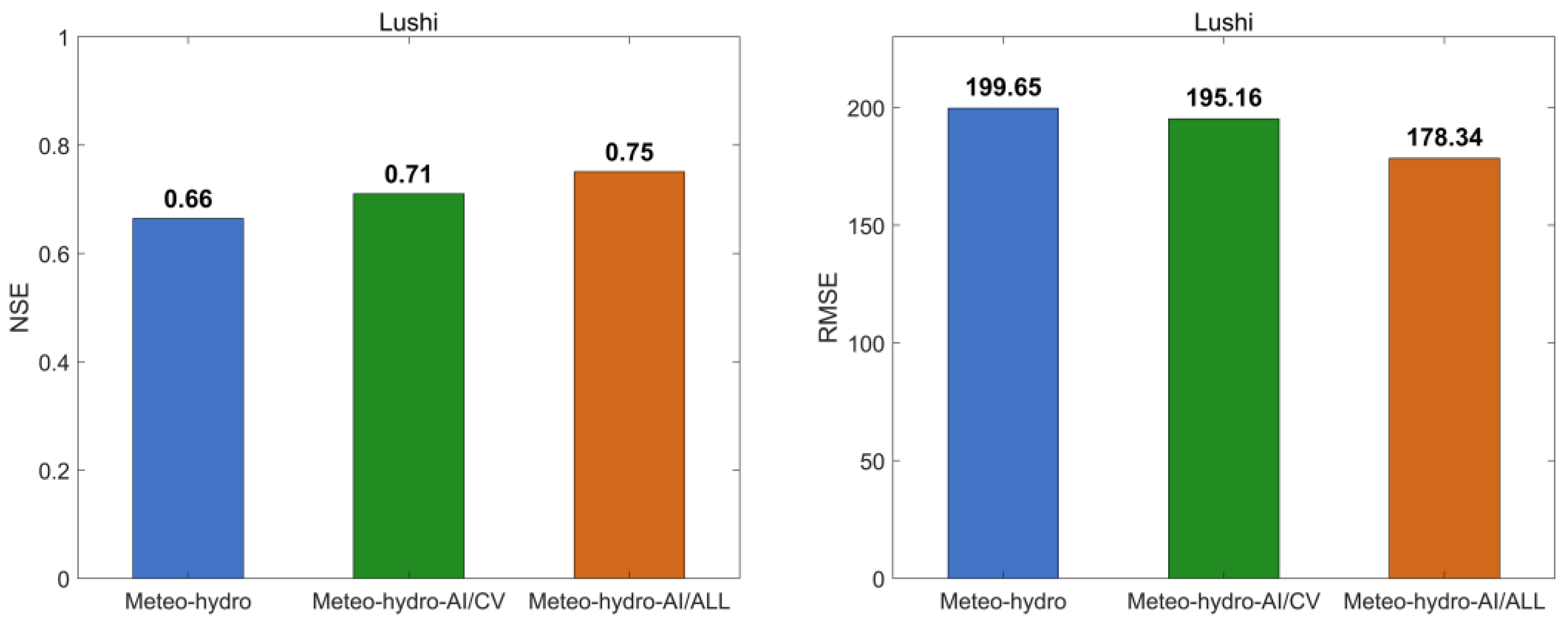
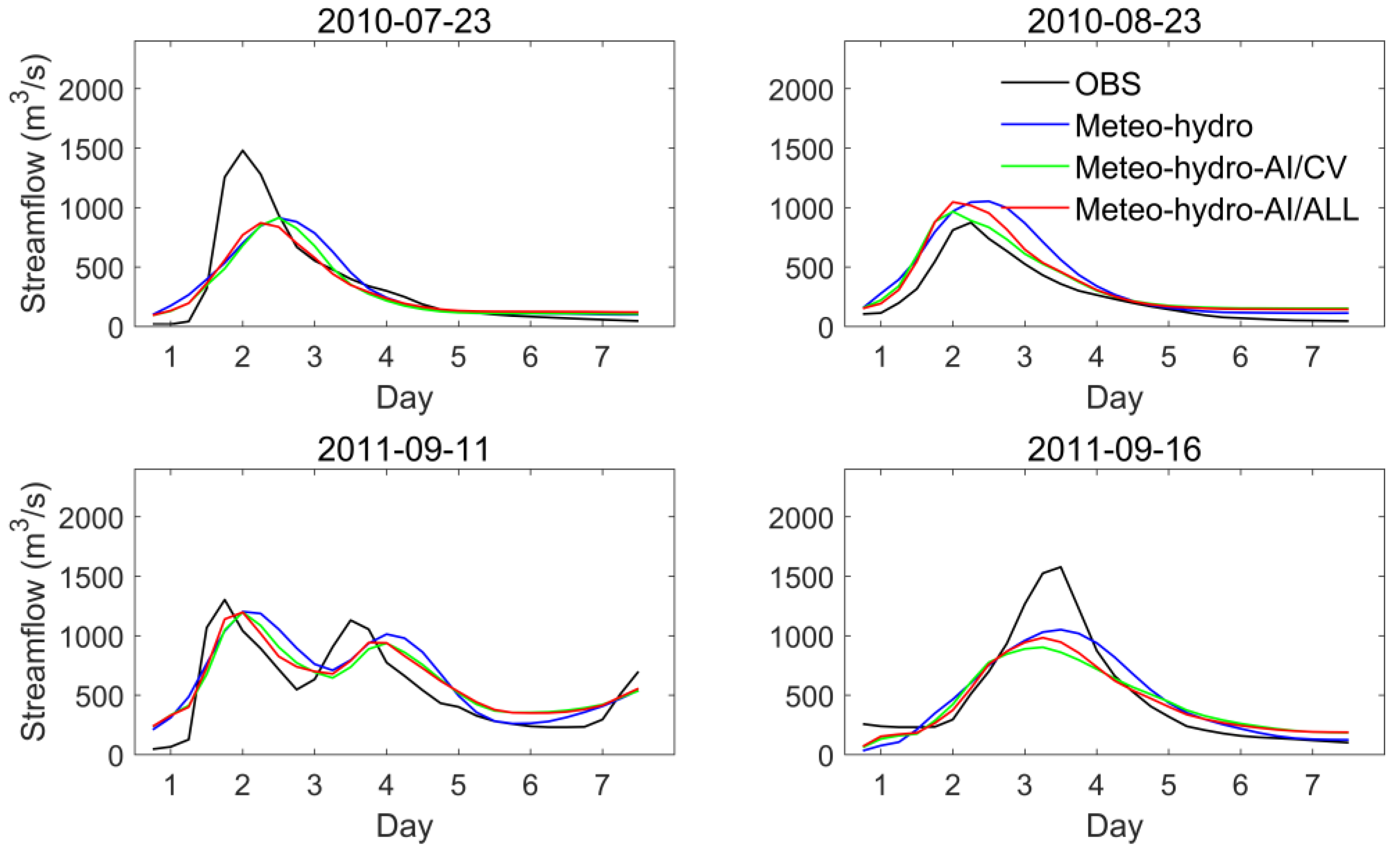
3.4. Correction of Meteo-Hydro Ensemble Forecast by LSTM Model

The deep learning method can learn characteristics, trends, and laws through datasets and can simulate or predict streamflow under the condition that the physical process is not clear. Figure 9 shows the ensemble mean streamflow forecasts from meteo-hydro and meteo-hydro-AI (combining meteo-hydro with the LSTM model) for extreme flood forecasts at the Lushi station. Compared with the meteo-hydro forecasts, meteo-hydro-AI corrects the lag of flood peaks to some extent (Figure 9).

The NSE and RMSE of the ensemble mean streamflow forecasts before and after LSTM correction are shown in Figure 10. Compared with the meteo-hydro forecasts, the NSE of meteo-hydro-AI/CV is increased by 0.05, and the RMSE is reduced by 2.2%. Without cross validation, the NSE can increase by 0.09, and RMSE can decrease by 11% (orange bars in Figure 10), which suggests the potential of the LSTM method. Further exploration is needed if the samples of extreme flood events are sufficient, but this is usually not the case since extreme events rarely occur.

3.5. Discussion

The “meteo-hydro” method is widely used in flood forecasting and has been extensively demonstrated in previous studies [9,56]. For instance, both GloFAS [30] (Global Flood Awareness System) and EFAS [57] (European Flood Awareness System) used this method to forecast flood events. We used the LSTM method to correct flood ensemble forecasts. However, the model’s training was insufficient due to the small number of extreme flood samples in the basins, which resulted in marginal improvement. The issue of “small sample” is common for most AI forecasting of extreme events.

There are additional approaches to fully explore the added values of applying deep learning techniques, e.g., using input upstream observations and downstream forecast results to train and correct the forecast [58], using multiple deep learning models, or migrating the research to a basin with more flooding data. Furthermore, this study did not consider reservoir operation. As deep learning techniques have shown their advantages in representing reservoir regulations [54], we expect that they could be applied to other aspects in future works (e.g., parameter estimation, physical parameterization scheme optimization, etc.), instead of being directly used in model post-processing.

The “meteo-hydro-AI” approach used in this study could be further improved and validated over tributaries, if more hydrological observation stations are employed. Though the ensemble meteorological forecast showed great superiority in flood forecasts against the traditional ESP method, the original forecast product from the global weather forecast model had a coarse spatial resolution, which made it a challenge to predict heavy precipitation at the local scale. Continued efforts are needed to develop high-resolution regional ensemble meteorological forecast systems for dynamical downscaling, explore suitable statistical downscaling methods, and use advanced data-assimilation methods to improve the predictive skills of extreme precipitation events [36,59,60,61], thereby enhancing the predictive skills of extreme floods.

4. Conclusions

In this study, we explored the added values of extreme flood forecasts by using ECMWF meteorological ensemble forecasts, CSSPv2 high-resolution land surface modeling, and the LSTM deep learning technique. The average NSE values for the hourly streamflow during the four extreme floods at the three interval sub-basins in the Luo River basin were 0.54, 0.55, and 0.66, respectively. This suggested that the CSSPv2 model performed well in simulating extreme floods. Compared to the ESP/CSSPv2 streamflow forecast, the ECMWF/CSSPv2 forecast demonstrated better reliability, lower false alarm rates, and higher hit rates in terms of probabilistic streamflow forecasts, with an average increase of 0.49 in NSE, and an average reduction in RMSE of 31.7%. Though the LSTM has potential to correct the forecasts, the improvement was marginal. This suggested a challenge in predicting extreme floods with deep learning techniques, as there were not enough samples for training.

The meteo-hydro-AI method proposed in this study can be easily implemented in local river basins without too much computational effort, as ECMWF weather forecasts are available globally. Future efforts could be devoted to improving forecasts of rainstorms with AI methods as well as dynamical downscaling from global weather forecasts, improving flood simulation by incorporating a hyper-resolution hydrodynamic module into the land surface model, and using more proxy data for improving flood forecasts with deep learning.

References

1. Yucel, I.; Onen, A.; Yilmaz, K.K.; Gochis, D.J. Calibration and evaluation of a flood forecasting system: Utility of numerical weather prediction model, data assimilation and satellite-based rainfall. J. Hydrol. 2015, 523, 49–66. [Google Scholar] [CrossRef]
2. Bodoque, J.M.; Díez-Herrero, A.; Eguibar, M.A.; Benito, G.; Ruiz-Villanueva, V.; Ballesteros-Cánovas, J.A. Challenges in paleoflood hydrology applied to risk analysis in mountainous watersheds—A review. J. Hydrol. 2015, 529, 449–467. [Google Scholar] [CrossRef]
3. Masson-Delmotte, V.; Zhai, P.; Pirani, A.; Connors, S.L.; Péan, C.; Berger, S.; Caud, N.; Chen, Y.; Goldfarb, L.; Gomis, M.I.; et al. (Eds.) IPCC, 2021: Summary for Policymakers. In Climate Change 2021: The Physical Science Basis. Contribution of Working Group I to the Sixth Assessment Report of the Intergovernmental Panel on Climate Change; Cambridge University Press: Cambridge, UK; New York, NY, USA, 2021; pp. 3–32. [Google Scholar]
4. Milly, P.C.D.; Betancourt, J.; Falkenmark, M.; Hirsch, R.M.; Kundzewicz, Z.W.; Lettenmaier, D.P.; Stouffer, R.J. Stationarity Is Dead: Whither Water Management? Science 2008, 319, 573–574. [Google Scholar] [CrossRef] [PubMed]
5. Alfieri, L.; Burek, P.; Feyen, L.; Forzieri, G. Global warming increases the frequency of river floods in Europe. Hydrol. Earth Syst. Sci. 2015, 19, 2247–2260. [Google Scholar] [CrossRef]
6. Yuan, X.; Ji, P.; Wang, L.; Liang, X.Z.; Yang, K.; Ye, A.; Su, Z.; Wen, J. High-Resolution Land Surface Modeling of Hydrological Changes Over the Sanjiangyuan Region in the Eastern Tibetan Plateau: 1. Model Development and Evaluation. J. Adv. Model. Earth Syst. 2018, 10, 2806–2828. [Google Scholar] [CrossRef]
7. Moradkhani, H.; Sorooshian, S.; Gupta, H.V.; Houser, P.R. Dual state–parameter estimation of hydrological models using ensemble Kalman filter. Adv. Water Resour. 2005, 28, 135–147. [Google Scholar] [CrossRef]
8. Yuan, X.; Wood, E.F. Downscaling precipitation or bias-correcting streamflow? Some implications for coupled general circulation model (CGCM)-based ensemble seasonal hydrologic forecast. Water Resour. Res. 2012, 48, W12519. [Google Scholar] [CrossRef]
9. Liu, J.; Yuan, X.; Zeng, J.; Jiao, Y.; Li, Y.; Zhong, L.; Yao, L. Ensemble streamflow forecasting over a cascade reservoir catchment with integrated hydrometeorological modeling and machine learning. Hydrol. Earth Syst. Sci. 2022, 26, 265–278. [Google Scholar] [CrossRef]
10. Chiang, Y.M.; Hsu, K.L.; Chang, F.J.; Hong, Y.; Sorooshian, S. Merging multiple precipitation sources for flash flood forecasting. J. Hydrol. 2007, 340, 183–196. [Google Scholar] [CrossRef]
11. Xiang, Z.; Yan, J.; Demir, I. A Rainfall-Runoff Model With LSTM-Based Sequence-to-Sequence Learning. Water Resour. Res. 2020, 56, e2019WR025326. [Google Scholar] [CrossRef]
12. Zhu, X.; Zhang, Y.; Qi, W.; Liang, Y.; Zhao, X.; Cai, W.; Li, Y. Flood forecasting methods for a semi-arid and semi-humid area in Northern China. J. Flood Risk Manag. 2022, 15, e12831. [Google Scholar] [CrossRef]
13. Bai, P.; Liu, X.M.; Xie, J.X. Simulating runoff under changing climatic conditions: A comparison of the long short-term memory network with two conceptual hydrologic models. J. Hydrol. 2021, 592, 125779. [Google Scholar] [CrossRef]
14. Liu, L.; Liu, X.; Bai, P.; Liang, K.; Liu, C. Comparison of flood simulation capabilities of a hydrologic model and a machine learning model. Int. J. Climatol. 2022, 43, 123–133. [Google Scholar] [CrossRef]
15. Liang, X.; Lettenmaier, D.P.; Wood, E.F.; Burges, S.J. A simple hydrologically based model of land surface water and energy fluxes for general circulation models. J. Geophys. Res. Atmos. 1994, 99, 14415–14428. [Google Scholar] [CrossRef]
16. Ciarapica, L.; Todini, E. TOPKAPI: A model for the representation of the rainfall-runoff process at different scales. Hydrol. Process. 2002, 16, 207–229. [Google Scholar] [CrossRef]
17. Kirchner, J.W. Getting the right answers for the right reasons: Linking measurements, analyses, and models to advance the science of hydrology. Water Resour. Res. 2006, 42, W03S04. [Google Scholar] [CrossRef]
18. De Graaf, I.E.M.; Sutanudjaja, E.H.; van Beek, L.P.H.; Bierkens, M.F.P. A high-resolution global-scale groundwater model. Hydrol. Earth Syst. Sci. 2015, 19, 823–837. [Google Scholar] [CrossRef]
19. Troin, M.; Arsenault, R.; Wood, A.W.; Brissette, F.; Martel, J.L. Generating Ensemble Streamflow Forecasts: A Review of Methods and Approaches Over the Past 40 Years. Water Resour. Res. 2021, 57, e2020WR028392. [Google Scholar] [CrossRef]
20. Day, G.N. Extended Streamflow Forecasting Using NWSRFS. J. Water Resour. Plan. Manag. 1985, 111, 157–170. [Google Scholar] [CrossRef]
21. Wood, A.W.; Lettenmaier, D.P. An ensemble approach for attribution of hydrologic prediction uncertainty. Geophys. Res. Lett. 2008, 35, L14401. [Google Scholar] [CrossRef]
22. Sabzipour, B.; Arsenault, R.; Brissette, F. Evaluation of the potential of using subsets of historical climatological data for ensemble streamflow prediction (ESP) forecasting. J. Hydrol. 2021, 595, 125656. [Google Scholar] [CrossRef]
23. Lorenz, E.N. Deterministic Nonperiodic Flow. J. Atmos. Sci. 1963, 20, 130–141. [Google Scholar] [CrossRef]
24. Leith, C.E. Theoretical Skill of Monte Carlo Forecasts. Mon. Weather Rev. 1974, 102, 409–418. [Google Scholar] [CrossRef]
25. Shutts, G. A kinetic energy backscatter algorithm for use in ensemble prediction systems. Q. J. R. Meteorol. Soc. 2006, 131, 3079–3102. [Google Scholar] [CrossRef]
26. Bauer, P.; Thorpe, A.; Brunet, G. The quiet revolution of numerical weather prediction. Nature 2015, 525, 47–55. [Google Scholar] [CrossRef]
27. Hopsch, S.B. Analysis of tropical high impact weather events using TIGGE data. In Proceedings of the 31st Conference on Hurricanes and Tropical Meteorology, San Diego, CA, USA, 31 March–4 April 2014. [Google Scholar]
28. Karuna Sagar, S.; Rajeevan, M.; Vijaya Bhaskara Rao, S.; Mitra, A.K. Prediction skill of rainstorm events over India in the TIGGE weather prediction models. Atmos. Res. 2017, 198, 194–204. [Google Scholar] [CrossRef]
29. Cloke, H.L.; Pappenberger, F. Ensemble flood forecasting: A review. J. Hydrol. 2009, 375, 613–626. [Google Scholar] [CrossRef]
30. Alfieri, L.; Burek, P.; Dutra, E.; Krzeminski, B.; Muraro, D.; Thielen, J.; Pappenberger, F. GloFAS—global ensemble streamflow forecasting and flood early warning. Hydrol. Earth Syst. Sci. 2013, 17, 1161–1175. [Google Scholar] [CrossRef]
31. Bennett, J.C.; Robertson, D.E.; Shrestha, D.L.; Wang, Q.J.; Enever, D.; Hapuarachchi, P.; Tuteja, N.K. A System for Continuous Hydrological Ensemble Forecasting (SCHEF) to lead times of 9 days. J. Hydrol. 2014, 519, 2832–2846. [Google Scholar] [CrossRef]
32. Bennett, J.C.; Wang, Q.J.; Pokhrel, P.; Robertson, D.E. The challenge of forecasting high streamflows 1–3 months in advance with lagged climate indices in southeast Australia. Nat. Hazards Earth Syst. Sci. 2014, 14, 219–233. [Google Scholar] [CrossRef]
33. Yuan, X.; Wood, E.F.; Ma, Z. A review on climate-model-based seasonal hydrologic forecasting: Physical understanding and system development. WIREs Water 2015, 2, 523–536. [Google Scholar] [CrossRef]
34. Wood, E.F.; Roundy, J.K.; Troy, T.J.; van Beek, L.P.H.; Bierkens, M.F.P.; Blyth, E.; de Roo, A.; Döll, P.; Ek, M.; Famiglietti, J.; et al. Hyperresolution global land surface modeling: Meeting a grand challenge for monitoring Earth’s terrestrial water. Water Resour. Res. 2011, 47, W05301. [Google Scholar] [CrossRef]
35. Zounemat-Kermani, M.; Batelaan, O.; Fadaee, M.; Hinkelmann, R. Ensemble machine learning paradigms in hydrology: A review. J. Hydrol. 2021, 598, 126266. [Google Scholar] [CrossRef]
36. Wang, Q.J.; Shao, Y.; Song, Y.; Schepen, A.; Robertson, D.E.; Ryu, D.; Pappenberger, F. An evaluation of ECMWF SEAS5 seasonal climate forecasts for Australia using a new forecast calibration algorithm. Environ. Model. Softw. 2019, 122, 104550. [Google Scholar] [CrossRef]
37. Govindaraju, R.S. Artificial Neural Networks in Hydrology. II: Hydrologic Applications. J. Hydrol. Eng. 2000, 5, 124–137. [Google Scholar]
38. Badrzadeh, H.; Sarukkalige, R.; Jayawardena, A.W. Impact of multi-resolution analysis of artificial intelligence models inputs on multi-step ahead river flow forecasting. J. Hydrol. 2013, 507, 75–85. [Google Scholar] [CrossRef]
39. He, Z.; Wen, X.; Liu, H.; Du, J. A comparative study of artificial neural network, adaptive neuro fuzzy inference system and support vector machine for forecasting river flow in the semiarid mountain region. J. Hydrol. 2014, 509, 379–386. [Google Scholar] [CrossRef]
40. Adnan, R.M.; Liang, Z.; Trajkovic, S.; Zounemat-Kermani, M.; Li, B.; Kisi, O. Daily streamflow prediction using optimally pruned extreme learning machine. J. Hydrol. 2019, 577, 123981. [Google Scholar] [CrossRef]
41. Yang, S.; Yang, D.; Chen, J.; Santisirisomboon, J.; Lu, W.; Zhao, B. A physical process and machine learning combined hydrological model for daily streamflow simulations of large watersheds with limited observation data. J. Hydrol. 2020, 590, 125206. [Google Scholar] [CrossRef]
42. Konapala, G.; Kao, S.-C.; Painter, S.L.; Lu, D. Machine learning assisted hybrid models can improve streamflow simulation in diverse catchments across the conterminous US. Environ. Res. Lett. 2020, 15, 104022. [Google Scholar] [CrossRef]
43. Cho, K.; Kim, Y. Improving streamflow prediction in the WRF-Hydro model with LSTM networks. J. Hydrol. 2022, 605, 127297. [Google Scholar] [CrossRef]
44. He, J.; Yang, K.; Tang, W.; Lu, H.; Qin, J.; Chen, Y.; Li, X. The first high-resolution meteorological forcing dataset for land process studies over China. Sci. Data 2020, 7, 25. [Google Scholar] [CrossRef] [PubMed]
45. Dai, Y.; Dickinson, R.E.; Wang, Y.-P. A Two-Big-Leaf Model for Canopy Temperature, Photosynthesis, and Stomatal Conductance. J. Clim. 2004, 17, 2281–2299. [Google Scholar] [CrossRef]
46. Choi, H.I.; Kumar, P.; Liang, X.Z. Three-dimensional volume-averaged soil moisture transport model with a scalable parameterization of subgrid topographic variability. Water Resour. Res. 2007, 43, W04414. [Google Scholar] [CrossRef]
47. Yuan, X.; Liang, X.-Z. Evaluation of a Conjunctive Surface–Subsurface Process Model (CSSP) over the Contiguous United States at Regional–Local Scales. J. Hydrometeorol. 2011, 12, 579–599. [Google Scholar] [CrossRef]
48. Yuan, F.; Xie, Z.; Duan, Q.; Zheng, J.; Liang, M.; Chen, F. Regional Parameter Estimation of the VIC Land Surface Model: Methodology and Application to River Basins in China. J. Hydrometeorol. 2007, 8, 447–468. [Google Scholar]
49. Hochreiter, S.; Schmidhuber, J. Long Short-Term Memory. Neural Comput. 1997, 9, 1735–1780. [Google Scholar] [CrossRef] [PubMed]
50. Hu, C.; Wu, Q.; Li, H.; Jian, S.; Li, N.; Lou, Z. Deep Learning with a Long Short-Term Memory Networks Approach for Rainfall-Runoff Simulation. Water 2018, 10, 1543. [Google Scholar] [CrossRef]
51. Hu, R.; Fang, F.; Pain, C.C.; Navon, I.M. Rapid spatio-temporal flood prediction and uncertainty quantification using a deep learning method. J. Hydrol. 2019, 575, 911–920. [Google Scholar] [CrossRef]
52. Mouatadid, S.; Adamowski, J.F.; Tiwari, M.K.; Quilty, J.M. Coupling the maximum overlap discrete wavelet transform and long short-term memory networks for irrigation flow forecasting. Agric. Water Manag. 2019, 219, 72–85. [Google Scholar] [CrossRef]
53. Chang, Z.; Zhang, Y.; Chen, W. Electricity price prediction based on hybrid model of adam optimized LSTM neural network and wavelet transform. Energy 2019, 187, 115804. [Google Scholar] [CrossRef]
54. Özdoğan-Sarıkoç, G.; Sarıkoç, M.; Celik, M.; Dadaser-Celik, F. Reservoir volume forecasting using artificial intelligence-based models: Artificial Neural Networks, Support Vector Regression, and Long Short-Term Memory. J. Hydrol. 2023, 616, 128766. [Google Scholar] [CrossRef]
55. Wilks, D.S. Statistical Methods in the Atmospheric Sciences, 3rd ed.; Elsevier Science: Amsterdam, The Netherlands, 2011; pp. 301–394. [Google Scholar]
56. Yuan, X.; Roundy, J.K.; Wood, E.F.; Sheffield, J. Seasonal Forecasting of Global Hydrologic Extremes: System Development and Evaluation over GEWEX Basins. Bull. Am. Meteorol. Soc. 2015, 96, 1895–1912. [Google Scholar] [CrossRef]
57. Thielen, J.; Bartholmes, J.; Ramos, M.-H.; de Roo, A. The European flood alert system—Part 1: Concept and development. Hydrol. Earth Syst. Sci. 2009, 13, 125–140. [Google Scholar] [CrossRef]
58. Ghimire, G.R.; Krajewski, W.F. Exploring persistence in streamflow forecasting. J. Am. Water Resour. Assoc. 2020, 56, 542–560. [Google Scholar] [CrossRef]
59. Li, W.; Chen, J.; Li, L.; Orsolini, Y.J.; Xiang, Y.; Senan, R.; de Rosnay, P. Impacts of snow assimilation on seasonal snow and meteorological forecasts for the Tibetan Plateau. Cryosphere 2022, 16, 4985–5000. [Google Scholar] [CrossRef]
60. Ravuri, S.; Lenc, K.; Willson, M.; Kangin, D.; Lam, R.; Mirowski, P.; Fitzsimons, M.; Athanassiadou, M.; Kashem, S.; Madge, S.; et al. Skilful precipitation nowcasting using deep generative models of radar. Nature 2021, 597, 672–677. [Google Scholar] [CrossRef]
61. You, Y.; Huang, C.; Wang, Z.; Hou, J.; Zhang, Y.; Xu, P. A genetic particle filter scheme for univariate snow cover assimilation into Noah-MP model across snow climates. Hydrol. Earth Syst. Sci. 2023, 27, 2919–2933. [Google Scholar] [CrossRef]
Figure 1. Locations of streamflow gauges and the Guxian reservoir over the Luo River basin in the middle reach of the Yellow River. The upper panel (a) shows the location of the Yellow River in China, panel (b) shows the location of the Luo River in the Yellow River, and the bottom panel (c) shows the Luo River.
Water 16 00990 g001
Figure 2. The experimental design. Here, only the meteo-hydro forecasts (i.e., CSSPv2 hydrological forecasts driven by ECMWF meteorological forecasts) were corrected by the LSTM deep learning model, because the skill of ESP forecasts is too low.
Water 16 00990 g002
Figure 3. Evaluation of the flood simulations at three hydrological stations along the mainstream of the Luo River basin. The black points and red lines are the observed and simulated hourly streamflow. The blue bars represent observed hourly precipitation. From the top to bottom panels, there are four floods at Lushi (ad), Yiyang (eh), and Baimasi (il) stations, respectively. The title of each panel represents the start date of the flood events, e.g., 2010-07-23 represents the flood that started on 23 July 2010.
Water 16 00990 g003
Figure 4. ECMWF ensemble precipitation forecasts (mm/6 h) during extreme flood events. The forecasts extend to seven days after the beginning of the floods. The box and gray shaded parts are ensemble precipitation forecasts, and the red and blue lines are ensemble mean predictions and observations of precipitation. The panels from top to bottom are the results of the Lushi (ad), Yiyang (eh), and Baimasi (il) interval basins, respectively.
Water 16 00990 g004
Figure 5. Evaluations of ECMWF/CSSPv2-based (meteo-hydro) ensemble flood forecasts. The box and gray shaded parts are ensemble flood forecasts, and the black and red lines are observations and average values of ensemble forecasts of streamflow. The panels from top to bottom are the results of the Lushi (ad), Yiyang (eh), and Baimasi (il) interval basins, respectively.
Water 16 00990 g005
Figure 6. The NSE and RMSE (m3/s) of ensemble flood forecasts from ESP and meteo-hydro approach. The statistics were averaged among the four selected extreme flood events for each hydrological station.
Water 16 00990 g006
Figure 7. Reliability diagram for ESP (a) and meteo-hydro (b) forecasts of extreme floods across three hydrological stations. The threshold for the diagram is the 99th percentile of the observed streamflow in 2010–2017. p ( y ) is the refinement distribution of forecast probability, and p ( o | y ) is the conditional distributions of the observation given each of the redistributed probability forecast ranges (e.g., 0–0.1, 0.1–0.2, etc.). The blue and black points/bar charts are the ESP and meteo-hydro forecasts.
Water 16 00990 g007
Figure 8. ROC diagrams for ESP and meteo-hydro ensemble flood forecasts for all extreme flood events at all three stations. The ROC threshold corresponds to the 99th percentile of the observed streamflow in 2010–2017. AUC is the area under the curve.
Water 16 00990 g008
Figure 9. Streamflow from observation and ensemble mean forecasts based on meteo-hydro and meteo-hydro-AI forecasts at Lushi station. The black, blue, green, and red lines are observed streamflow, meteo-hydro streamflow forecasts, and meteo-hydro-AI streamflow forecasts with (CV) or without (ALL) cross validation. The cross validation is performed by excluding the target flood event and training the LSTM model with the other three flood events.
Water 16 00990 g009
Figure 10. NSE and RMSE (m3/s) of the ensemble flood forecasts from meteo-hydro and meteo-hydro-AI with (CV) or without (ALL) cross validation.
Water 16 00990 g010