Infiltration-Based Variability of Soil Erodibility Parameters Evaluated with the Jet Erosion Test

Abstract

Soil erosion by water on agricultural hillslopes leads to numerous environmental problems including reservoir sedimentation, loss of agricultural land, declines in drinking water quality, and requires deep understanding of underlying physical processes for better mitigation. It is imperative to accurately predict soil erosion caused by overland flow processes so that soil conservation efforts can be undertaken proactively before large-scale sedimentation problems arise. Soil detachment is often described by the excess shear stress equation that contains two physical soil erodibility parameters, erodibility coefficient, and critical shear stress. These parameters are normally assumed to be constant but can change across varying soil texture classes as well as during surface runoff events due to changes in soil cohesion and potential dependency on soil moisture content. These changes may significantly affect soil erosion rates at the field and watershed scale. In this study, the erodibility parameters of three soil types (sandy loam, clay loam, and silty clay loam) were analyzed using a laboratory mini-Jet Erosion Test (JET) to determine the effect of soil sample infiltration and moisture condition. Results from the experiments depicted a dynamic relationship between the soil erodibility parameters and amount of infiltrated mass of water. Data analysis displayed that for soils of different texture critical shear stress exhibited local minimum with higher values for very dry and saturated soils, while erodibility coefficient tended to increase with the increase of mass of soil water. Utilizing these dynamic soil erodibility parameters did not result in a significant difference in soil erosion rates when compared to using the averaged soil erodibility parameters taken from the experiment but the range of potential erosion rates increases with the increase of applied sheer stress to soil surface. The erosion rates with the experiment-based coefficients were found to be higher than with the baseline WEPP-based coefficients. These results highlight the importance of evaluating the effect of intrastorm dependent factors during surface runoff events, such as antecedent soil moisture content, time to peak from the start of runoff, soil cohesion, etc., on soil erodibility parameters to accurately calculate erosion rates, especially for initially dry soils or during earlier stages of surface runoff when critical shear stresses were highly affected. Further assessment of such factors with JET or other laboratory and field tests is recommended.

1. Introduction

Soil erosion by water accounts for more than half of all soil erosion on U.S. cropland with an estimated 980 million Mg of topsoil lost in 2017 to sheet and rill erosion alone (https://www.nrcs.usda.gov/nri, accessed on 1 February 2024; [1]). Soil erosion leads to numerous environmental problems including reservoir and stream sedimentation, loss of agricultural land, and declines in drinking water quality [2,3]. It is imperative to accurately predict soil erosion caused by runoff processes so that mitigation efforts can be undertaken proactively before large-scale sedimentation and water quality problems arise.

Soil detachment by water is often described by the excess shear stress Equation (1):

$$\epsilon =k_d{\left(\tau -{\tau }_c\right)}^a$$

(1)

where $\epsilon$ is the rate of soil loss (ms⁻¹), $\tau$ is the applied hydraulic stress (Pa), $k_d$ is the erodibility coefficient (${\mathrm{m}}^3$N⁻¹s⁻¹), ${\tau }_c$ is the critical shear stress (Pa), and a ($\ge 1$) is an empirical exponent very often assumed to be unity [4,5]. Soil erosion is zero if hydraulic stresses are smaller than the critical shear stress ($\epsilon =0$ if $\tau <{\tau }_c$).

Some experimental techniques for quantifying soil erodibility parameters in Equation (1) include open channel erosion tests conducted in a flume [6], monitoring soil erosion in field plots [7], and repeated measurements of erosion pins [8]. The implementation of these methods is expensive in terms of cost, labor, and time; thus, alternative experimental methods can be considered. 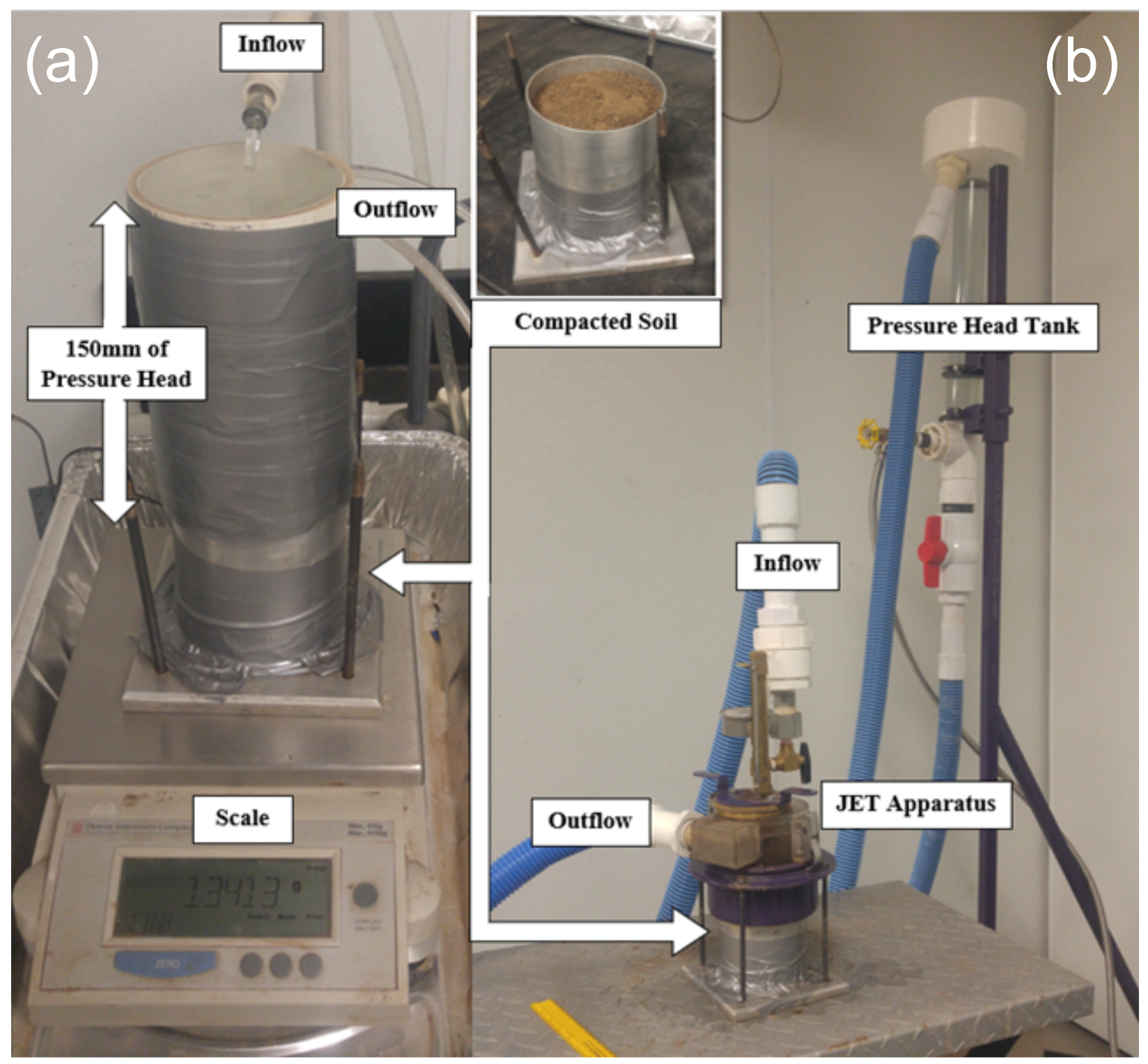One such alternative laboratory technique for estimating soil erodibility parameters utilizes a circular jet testing technique pioneered by Hanson and Cook [9] and further developed into a jet erosion test apparatus [6,10]. The Jet Erosion Test (JET) is a laboratory experiment that uses an apparatus to apply an impinging jet of water into a soil sample and create a scour. Based on the recorded scour depth over time during the test and using the characteristics of the experimental setup (such as nozzle velocity, pressure head, and discharge coefficient), an analytical approximation of the shear stress relationship applied at the soil sample’s surface can be derived. This approximation takes the form of a non-linear scour depth equation that can be solved for best fit values of $k_d$ and ${\tau }_c$ using mathematical optimization approaches [9,11]. A popular approach is the solution based on work by Blaisdell et al. [12], which applies a hyperbolic function to better fit the observed scour depth over time by adjusting values of the coefficients $k_d$ and ${\tau }_c$.

The accuracy of the derived soil erodibility parameters was evaluated by Hanson and Cook [6] who concluded that the JET method was a comparable method to established methods (open channel flumes). However, the results of JET experiments can have a high degree of variability in estimating $k_d$ and ${\tau }_c$. The variability can be attributed to many factors including a variability of soil samples, soil sample preparation techniques, operation of the JET experiment, size of sample mold, and parameter estimation solution approaches. A study by Liu et al. [13] evaluated soil erodibility parameters for three soils (sandy loam with 69% sand, silt loam with 72% silt, and silty clay with 39% clay) and five initial soil water conditions. The results for the studied soils showed that both parameters were affected by soil texture, pore void ratio, and soil water potential. Khanal et al. [14] conducted numerous JET experiments on two streambank soils and evaluated the impacts of user-controlled experiment parameters, such as, hydraulic pressure head, initial interval of scour depth measurement, and termination time. It was found that combinations of the factors were more important for variability of experiment outcomes than the impact of the sole factors, and the impact increased at larger head settings.

Soil erodibility parameters $k_d$ and ${\tau }_c$ in Equation (1) are normally assumed constant and dependent only on soil pedology factors. As an example, in a widely used soil erosion model WEPP (The Water Erosion Prediction Project [15,16]), the main dependent factors include texture, organic matter, and particle size distribution. Lisenbee et al. [17] compared the results of JET experiments for soils of tallgrass prairie and red ceder woodlands with the estimates from the WEPP model under varying soil conditions and found out that the WEPP-based $k_d$ were smaller that JET-derived values, while the values of ${\tau }_c$ were within the same order of magnitude. In addition, laboratory and field studies have shown that these parameters may vary with the changes in soil moisture content and pore pressure gradients that occur during rainfall, surface runoff, and/or soil infiltration events [3,13,18,19,20,21,22,23].

The JET apparatus was used in several studies to assess the impact of soil water states on soil erodibility [13,20,23,24]. For example, Hanson and Hunt [24] investigated the effects of compaction and soil moisture in loam and sandy loam soils using a laboratory JET device and concluded a curvelinear relationship between the erodibility coefficient and a sample water content with its minimum value representing lowest rate of soil erosion. Recent work by Khanal et al. [23] investigated the impact of soil moisture on the derived soil erodibility parameters of clay loam and sandy loam soils utilizing the mini-JET apparatus and varying soil moisture contents of the samples using an apparatus that simulated the infiltration process. It was concluded that as soil moisture increased, $k_d$ and ${\tau }_c$ also increased. In addition to initial water content, the effect of seepage forces on soil erodibility was evaluated in [20] and yielded that the observed scour depth increased, the critical shear stress decreased, and the erodibility coefficient increased when a soil was exposed to increasing seepage forces during the experiment.

The effects of soil moisture and dynamic pore pressure gradients on soil erodibility parameters were apparent in other methods of estimating soil erodibility parameters as well. A study investigating the effect of seepage on soil erodibility using a V-shaped flume discovered that a soil exhibited higher erodibility when it was under seepage conditions as opposed to drainage conditions [19]. Additionally, a laboratory study of clay-type soils in Texas using a rotating-cylinder test apparatus found a negative linear relationship between the critical shear stress, ${\tau }_c$, and soil moisture content [25]. That study observed a decrease of 50% in ${\tau }_c$ for a 15% increase in soil moisture content. A field study in central Kansas on ephemeral gully evolution in a silty clay soil found out that intrastorm dynamics of subsurface soil moisture play an important role in channel development and erosion rate estimates [21,22]. It was concluded that runoff events with lower antecedent soil moisture condition caused smaller soil erosion rates compared to the events with fully saturated soil.

The evidence from the previous studies showed the varying impact of soil water on shear strength and cohesiveness of soils. The positive effect refers to increased cohesiveness, improved soil resistance to scour and reduced erosion rates as evidenced, for example, by Huang and Laften [26] and Khanal et al. [23]. The negative effect relates to weakening of interparticle binding forces, enhanced particle detachment due to applied shear, and increased erosion rates [27]. The dynamic effects of time-dependent soil moisture content and its variability with depth during rainfall events, affected pore pressure gradients, and seepage and subsurface flows are not well understood and require additional attention from experimental and modeling studies. Thus, it becomes vital to understand how these effects can be quantified over a wide range of soil texture classes and under different soil water profiles. Therefore, the objective of this study was to evaluate the dynamic effects of infiltration on the erodibility coefficient and critical shear stress for representative soils on agricultural fields using the JET technique. We focused on soils with different soil texture and organic matter content collected from rangeland and cultivated cropland fields under conventional tillage and no-till practices.

2. Materials and Methods

2.1. Soil Properties

Three soils from agricultural fields in Kansas were utilized for this study [28,29]. All soils were extracted undisturbed from the near soil surface to a depth of approximately 30 cm. Soil texture, organic matter, and bulk density were analyzed in a soil testing laboratory and presented in

Table 1. Summary of the properties of three studied soils [31].

ID	Landuse	Management	Texture Class	Sand %	Silt %	Clay %	Organic Matter %	Soil Density Mg m−3
I	Cropland	Tilled	Silty clay loam	16	48	36	4.25	1.45
II	Pasture	Grazed	Clay loam	38	32	30	4.13	1.49
III	Cropland	No-till	Sandy loam	74	14	12	1.37	2.08

[30,31]. Soil I was a silty clay loam collected from a tilled cropland field north of Manhattan, Kansas. Soil II was a clay loam taken from pastureland north of Perry, Kansas that had over 40 years of cattle grazing. Soil III was a sandy loam collected from a no-till cultivated cropland field near McPherson, Kansas. Organic matter content varied among the soils, with a higher percentage found in soils I and II. Sandy loam soil III had lower below ground biomass that resulted in higher bulk density.

2.2. Soil Preparation

For each soil, after field soil collection, soil was stored away from direct sunlight and at room temperature, transported to the laboratory, and prepared for the infiltration experiment. The soils were air dried and filtered using a standard size sieve No. 4 (4.75 mm) to eliminate large foreign materials. To achieve the desired 5% soil moisture content, each sieved soil was initially weighed, oven dried at 95 °C for 24 h to remove all gravitational water, and then had different quantities of water uniformly applied. The soil was then allowed to settle undisturbed in a closed container to allow moisture distribution to reach equilibrium after 24 h. A standard cylindrical mold (height of 12 cm; diameter of 10.16 cm; volume of 972 ${\mathrm{cm}}^3$) was used for the experiments. A water-tight liner was attached to the bottom of the standard mold to minimize water leakage and the entire assembly was attached to a metal base plate (Figure 1a). In accordance with ASTM Standard D698 [32], the prepared soil of 5% soil moisture content was added to the mold in three layers; each layer was compacted by manually dropping a rammer of 2.5 kg in weight 25 times from a height of 30 cm producing a compactive effort of about 600 kN m m⁻³.

With the soil compacted in the mold, a standard US size 40 mesh with 0.425 mm opening and a grade 4 filter paper (pore size of ∼25 $\mathsf{\mu }$m) were placed on top of the sample to prevent soil particles from being disturbed during the infiltration experiment.

2.3. Soil Infiltration

An infiltration apparatus was designed and placed on top of the mold with the comp acted soil as shown in Figure 2a. The infiltration apparatus was constructed from a PVC pipe, two outflow tubes, and a water supply line that provided a continuous water influx. Initially the infiltration apparatus and mold (containing the soil sample) were separated by impermeable plastic membrane to prevent water infiltrating into the soil during the initial stage of filling the apparatus. The mold and empty infiltration apparatus were attached vertically and placed on a scale to monitor the change in weight. Then water was allowed to flow in and fill the apparatus to a 150 mm depth; any water above that depth was transferred out of the system through the outflow tube. When the inflow equaled the outflow, the system had reached equilibrium, and the scale was tared to set a reference point for the mass of infiltrated water. At this point, the plastic membrane separating the mold and the infiltration apparatus was penetrated and water was allowed to infiltrate into the soil. The infiltration process continued until the desired mass of water was reached on the scale. After that, the inflow stopped, and the apparatus was promptly disassembled from the mold. Once the mold was detached, it was placed horizontally to prevent any additional vertical redistribution of soil moisture into the sample and was ready for the JET.

2.4. Soil Moisture

For each soil, four to five infiltration experiments with different total masses of infiltrated water were conducted to evaluate a distribution of soil moisture in the core at different times and infiltration depths. Since the water level of the infiltration apparatus was always maintained at the same height of 150 mm during each experiment, soil moisture distribution with different masses of infiltrated water can be seen as representing an infiltration process at different times with a constant ponding depth. To observe the distribution of water in the soil following the infiltration procedure, three equally distributed soil cores (approximately 2 cm in diameter and 12 cm in length) were taken from each soil sample (Figure 1b,c). Each soil core was cut into 1 cm segments, and each segment was weighed, and oven dried at 95 °C for 24 h. The weight difference in each segment before and after the drying provided soil moisture distribution in the core.

2.5. Jet Erosion Test

The utilized mini-JET apparatus (Figure 2b) consisted of the following main parts: a pressure head tank, water inflow and outflow, a submergence tank (soil specimen and standard mold), and a nozzle and depth gauge connected to a rotating plate [10]. The nozzle on the rotating plate allowed the impinging jet of water to be disconnected from the soil specimen while still providing a constant water level in the submergence tank. The JET apparatus was connected to the pressure head tank by the inflow pipe and to a drain by the outflow pipe. The pressure head tank, while connected to a continuous water source, provided a consistent flow of water to maintain the pressure head of each test at 91 cm (36 in) for soils I and II and 122 cm (48 in) for soil III. The mold with a variable moisture soil sample was attached to the JET apparatus.

The JET was conducted on the soil sample immediately after the conclusion of the infiltration experiment. At the beginning of each test, a valve was opened to allow water from the pressure head tank to submerge the compacted soil. Once submerged, the depth gauge was used to find the point of reference for the scour hole. At each subsequent step, the nozzle was opened for a specified time interval and the scour depth was measured with the depth gauge. This procedure continued with gradually increasing time intervals until scour depth did not change for at least two periods, and equilibrium scour depth was reached.

2.6. Blaisdell Solution for Soil Erodibility Parameters

The soil erodibility parameters were determined by analyzing the scour depth recordings with the Blaisdell solution approach [6,12] using the spreadsheet tool developed by Daly et al. [11]. The approach uses Equation (1) to calculate jet scour depth assuming shear stress applied by the jet is maximum at the soil surface, thus forcing scour to grow rapidly at the beginning of the experiment. With time the rate reduces and, eventually, tends to zero when the equilibrium scour depth is reached.

The parameters of the experimental setup and the apparatus (Figure 2), such as, jet nozzle diameter $d_0$ and velocity $U_0$, the distance from jet origin to the initial soil surface in the mold are incorporated in model derivation. The mathematical form for the change in scour depth with time is represented by a non-linear algebraic equation:

$$t=t_r\left(0.5logy\left(H\right)-0.5logy\left(H_p\right)+H_p-H\right),y\left(H\right)=\frac{1+H}{1-H}$$

(2)

where t is measured time since beginning of the scour, $t_r=z_e/k_d{\tau }_c$ is the reference equilibrium time, $H=z/z_e$ is the scour depth at time t normalized to the equilibrium depth $z_e$, and $H_p=C_d{d}_0/z_e$, $C_d=6.3$ is the diffusion coefficient.

Since reaching the equilibrium can take a long time, and the equilibrium depth $z_e$ is unknown, Blaisdell et al. [12] proposed to use the following hyperbolic form equation to approximate $z_e$ and the corresponding time:

$${(f-f_0)}^2-x^2=N^2$$

(3)

where $f=log(z/d_0)-x$, $x=log(U_{0}t/d_0)$, and coefficients $f_0=log(z_e/d_0)$, and N are the fitting coefficients. Equations (2) and (3) are solved iteratively by minimizing the error with the measured scour depth dataset at fitting the coefficients $f_0$ and N and re-calculating $k_d$ and ${\tau }_c$ at each iteration. The solver in Daly et al. [11] provides an automatic way of generating best-fit values of ${\tau }_c$ and $k_d$ for the Blaisdell’s approach.

2.7. WEPP-Based Erodibility Parameters

The mechanistic soil erosion model in the Water Erosion Prediction Project (WEPP; [15,16,17]) represents $k_d$ and ${\tau }_c$ as products of baseline coefficients ($k_d^{WEPP}$, ${\tau }_c^{WEPP}$) and additional fractional adjustment terms ($k_{adj}^{WEPP}$, ${\tau }_{adj}^{WEPP}$):

$$k_d=k_d^{WEPP}{k}_{adj}^{WEPP}$$

(4)

$${\tau }_c={\tau }_c^{WEPP}{\tau }_{adj}^{WEPP}$$

(5)

The additional terms in Equations (4) and (5) adjust the parameters for specific natural conditions to account for soil residue, live and dead plant roots, soil sealing and crusting, and the impact of freeze/thaw cycles. In the case of laboratory mini-JET experiments, the soil was prepared bare, free of vegetation, and not subjected to freeze/thaw and other factors. Thus, the adjustments to baseline conditions were not applied and assumed that $k_{adj}^{WEPP}=1$ and ${\tau }_{adj}^{WEPP}=1$.

Baseline $k_d^{WEPP}$ and ${\tau }_c^{WEPP}$ are presented as functions of sand, clay, organic matter content orgmat, and dry soil bulk density ${\rho }_b$ for cropland and rangeland as

$$k_d^{WEPP}=\left\{\begin{array}{ccc}0.0069+0.134e^{-20\mathit{clay}},\hfill & \mathrm{i}\mathrm{f} \mathit{sand}\le 30\%\hfill & \mathrm{f}\mathrm{o}\mathrm{r} \mathrm{c}\mathrm{r}\mathrm{o}\mathrm{p}\mathrm{l}\mathrm{a}\mathrm{n}\mathrm{d}\hfill \\ 0.00197+0.03\mathit{sand}+0.03863e^{-184\mathit{orgmat}},\hfill & \mathrm{i}\mathrm{f} \mathit{sand}>30\%\hfill & \mathrm{f}\mathrm{o}\mathrm{r} \mathrm{c}\mathrm{r}\mathrm{o}\mathrm{p}\mathrm{l}\mathrm{a}\mathrm{n}\mathrm{d}\hfill \\ 0.0017+0.0024\mathit{clay}-0.0088(\mathit{orgmat}-0.0001{\rho }_b),\hfill & \mathrm{f}\mathrm{o}\mathrm{r} \mathrm{r}\mathrm{a}\mathrm{n}\mathrm{g}\mathrm{e}\mathrm{l}\mathrm{a}\mathrm{n}\mathrm{d}\hfill \end{array}\right.$$

(6)

$${\tau }_c^{WEPP}=\left\{\begin{array}{ccc}3.5,\hfill & \mathrm{i}\mathrm{f} \mathit{sand}\le 30\%\hfill & \mathrm{f}\mathrm{o}\mathrm{r} \mathrm{c}\mathrm{r}\mathrm{o}\mathrm{p}\mathrm{l}\mathrm{a}\mathrm{n}\mathrm{d}\hfill \\ 2.67+6.5\mathit{clay}-5.8\mathit{sand},\hfill & \mathrm{i}\mathrm{f} \mathit{sand}>30\%\hfill & \mathrm{f}\mathrm{o}\mathrm{r} \mathrm{c}\mathrm{r}\mathrm{o}\mathrm{p}\mathrm{l}\mathrm{a}\mathrm{n}\mathrm{d}\hfill \\ 3.23-5.6\mathit{sand}-24.4\mathit{orgmat}+0.0009{\rho }_b,\hfill & \mathrm{f}\mathrm{o}\mathrm{r} \mathrm{r}\mathrm{a}\mathrm{n}\mathrm{g}\mathrm{e}\mathrm{l}\mathrm{a}\mathrm{n}\mathrm{d}\hfill \end{array}\right.$$

(7)

The formulations in Equations (6) and (7) were applied to soils I, II, and III in Table 1 to calculate $k_d^{WEPP}$ and ${\tau }_c^{WEPP}$.

3. Results

3.1. Soil Moisture Distribution

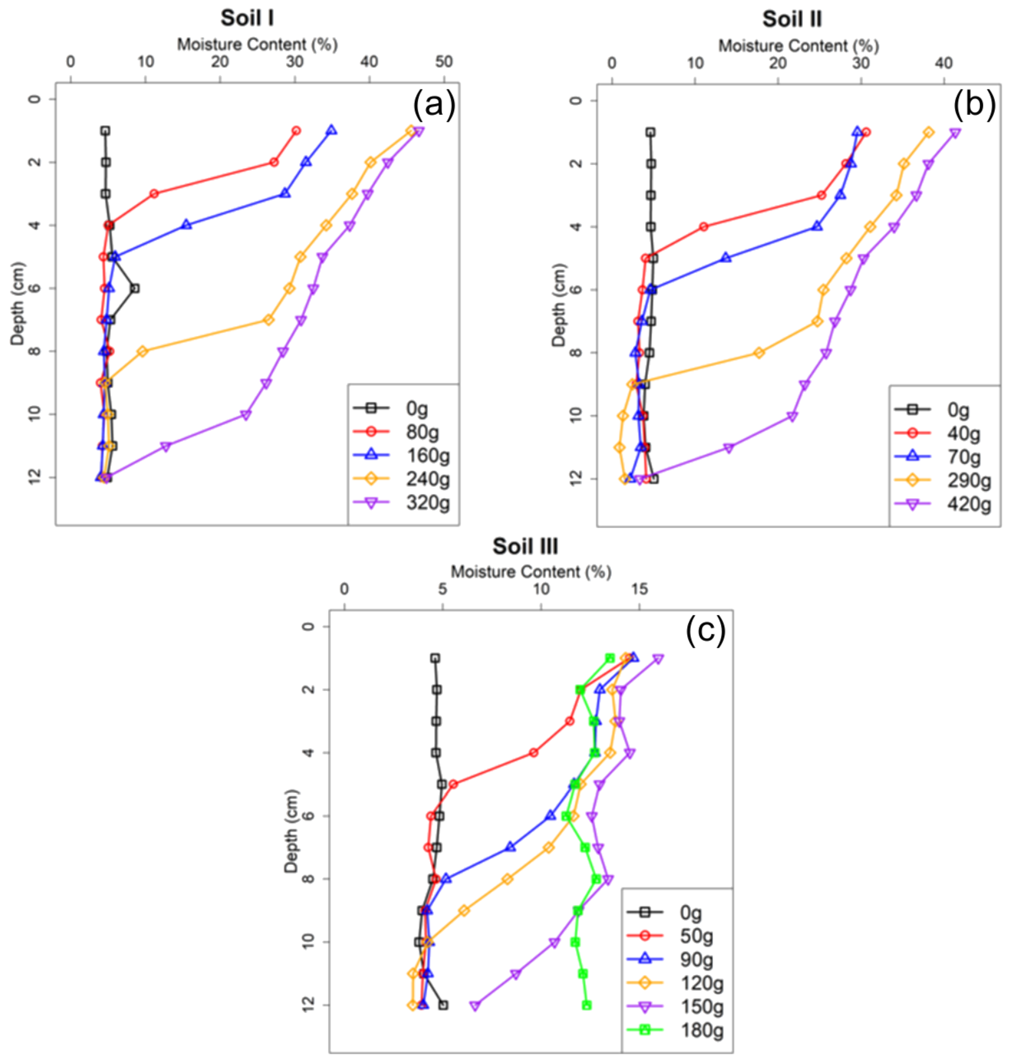
The infiltration experiment was repeated three times for each mass of infiltrated water for each soil. Five amounts of water (in grams) were infiltrated in soil I (0, 80, 160, 240, 320 g) and soil II (0, 40, 70, 290, 420 g) while six different masses were selected for soil III (0, 50, 90, 120, 150, 180 g). 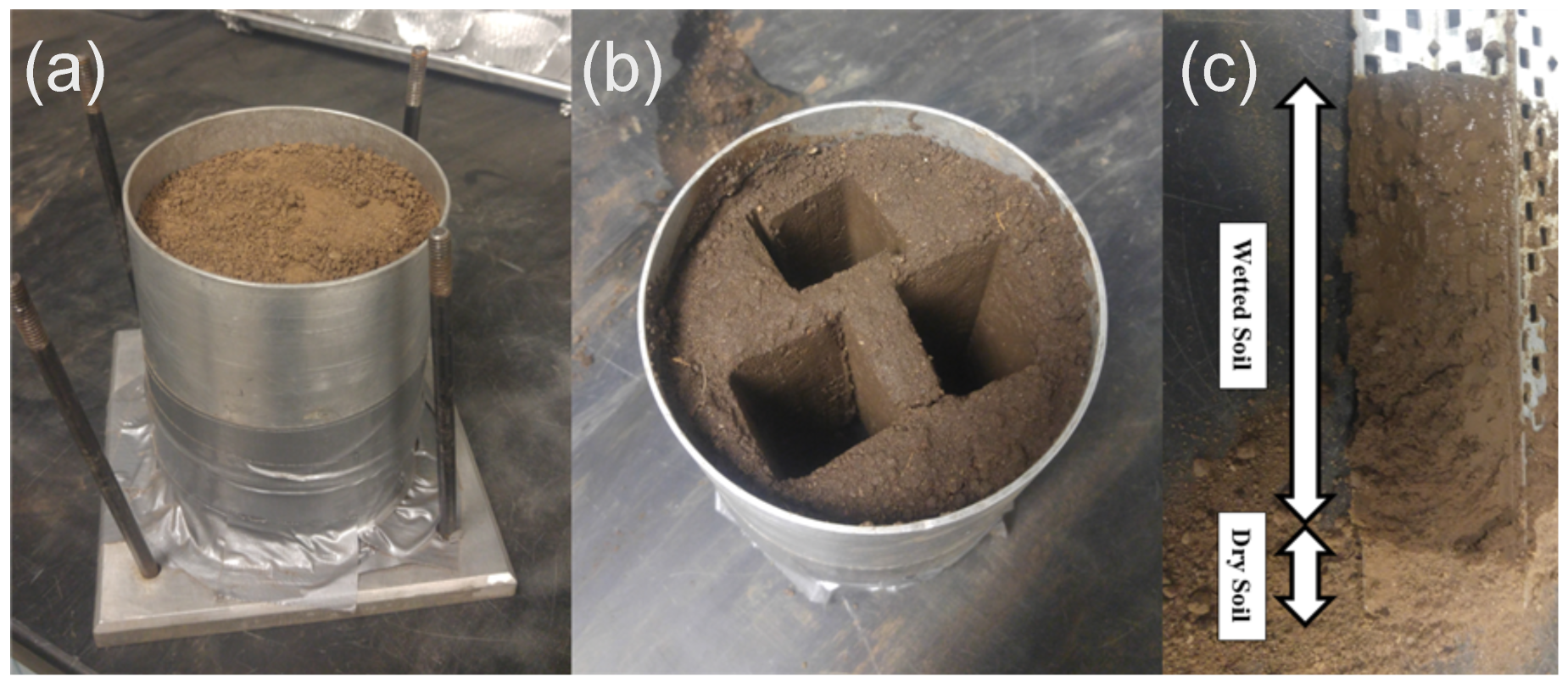For each experiment, a soil moisture content distribution with depth was developed, and average values of three samples at each depth were calculated (Figure 3). The curves followed a typical infiltration profile with saturation decreasing from the highest value at the top to near initial saturation at the bottom with the wetting front caused by the infiltrated mass of water clearly identifiable. At later times of infiltration, gravity was the primary controlling force and caused water to accumulate at lower depths because of a no flow boundary condition at the bottom. Saturation at the top of the sample was determined at a depth of 1 cm; however, it can be inferred that the top boundary was at full saturation due to the presence of ponded water in the JET apparatus during the tests.

Soil I had the slowest infiltration rate by infiltrating higher amounts of water within the same time periods. This is due to its lower hydraulic conductivity and higher organic matter content compared to the other soils. Soil III had the highest sand fraction of all three soils at 74% and the highest hydraulic conductivity, which manifested in a faster percolation of water through the soil profile compared to soils I and II. Overall, before water ponded on the bottom, and the sample became fully saturated, soil II infiltrated the highest amount of water at 420 g, while soil III had the least amount of water at 150 g.

3.2. Scour Depth with Time

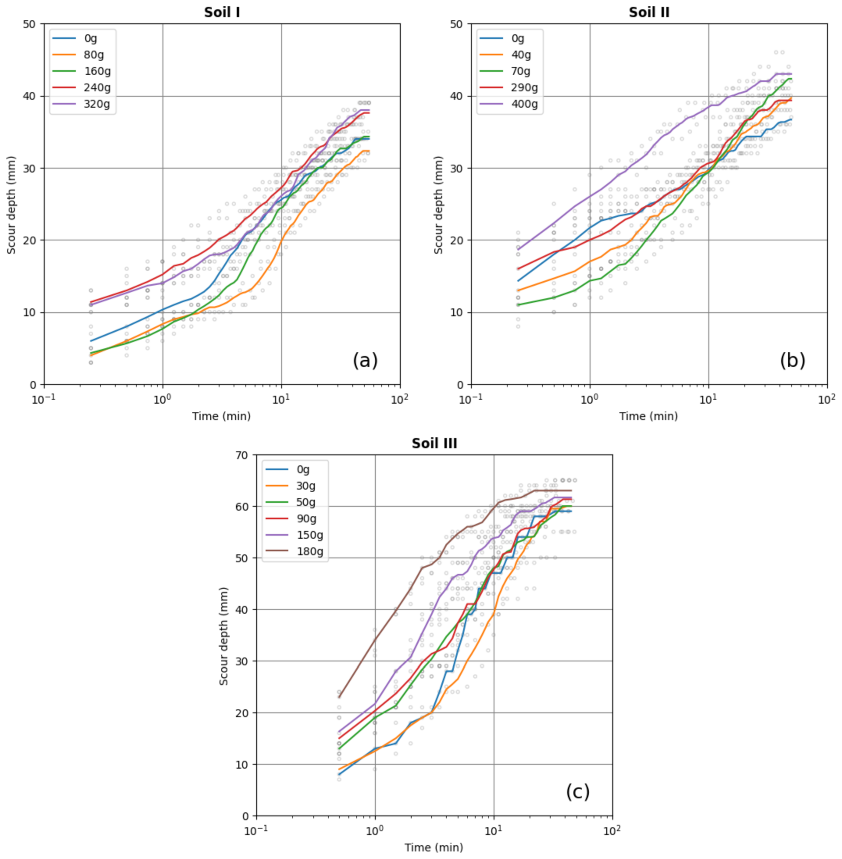
Similar to the infiltration experiment, five different masses (in grams) of infiltrated water were selected for soil I (0, 80, 160, 240, 320) and soil II (0, 40, 70, 290, 420), and seven different masses for soil III (0, 30, 50, 90, 120, 150, 180). The JET experiment was repeated three times for each mass of infiltrated water for each soil, with exceptions for soil III (0 g, one experiment; 30 g, two experiments). A total of 45 JET experiments were conducted with the samples of different infiltrated masses of water.

In each JET experiment, scour depth was recorded at 15 s to 5 minute intervals [28,29]. At the initial stage of the experiment, observed scour increased rapidly, which required smallest intervals between measurements (i.e., 15 s). Once the mold became more saturated, the recording interval was gradually increased to 5 min. The experiment ended when no changes were recorded for at least two consecutive 5 min intervals and the equilibrium depth was assumed reached.

Scour depth measurements are presented in a log time scale in Figure 4 as gray open circles for all experiments, while the average depths were shown as solid lines for molds with different masses of infiltrated water. The scour rates were the highest at the beginning and reduced to zero at the end of the experiment. The average time to reach the equilibrium depth varied from 34 to 55 min, with soil II having the fastest rates. The final scour depths varied from 32 mm for 80 g in soil I to 65 mm for 180 g in soil III. On average, for all infiltrated mass of water, soil I produced the smallest scours and soil III showed the highest scour depths.

In each experiment, samples with smaller amounts of infiltrated water produced smaller scours at the beginning of the experiment and then mostly maintained the difference with time than the samples with higher amounts of infiltrated water (i.e., see orange curve vs purple curve). Initially dry samples (0 g infiltrated mass, blue curves) had higher scours than the slightly wet samples (80 g, 160 g for soil I; 40 g, 70 g for soil II; 30 g for soil III) but lower scours than the fully wet samples (240 g, 320 g for soil I; 290 g, 400 g for soil II; 150 g, 180 g for soil III).

3.3. Soil Erodibility Parameters

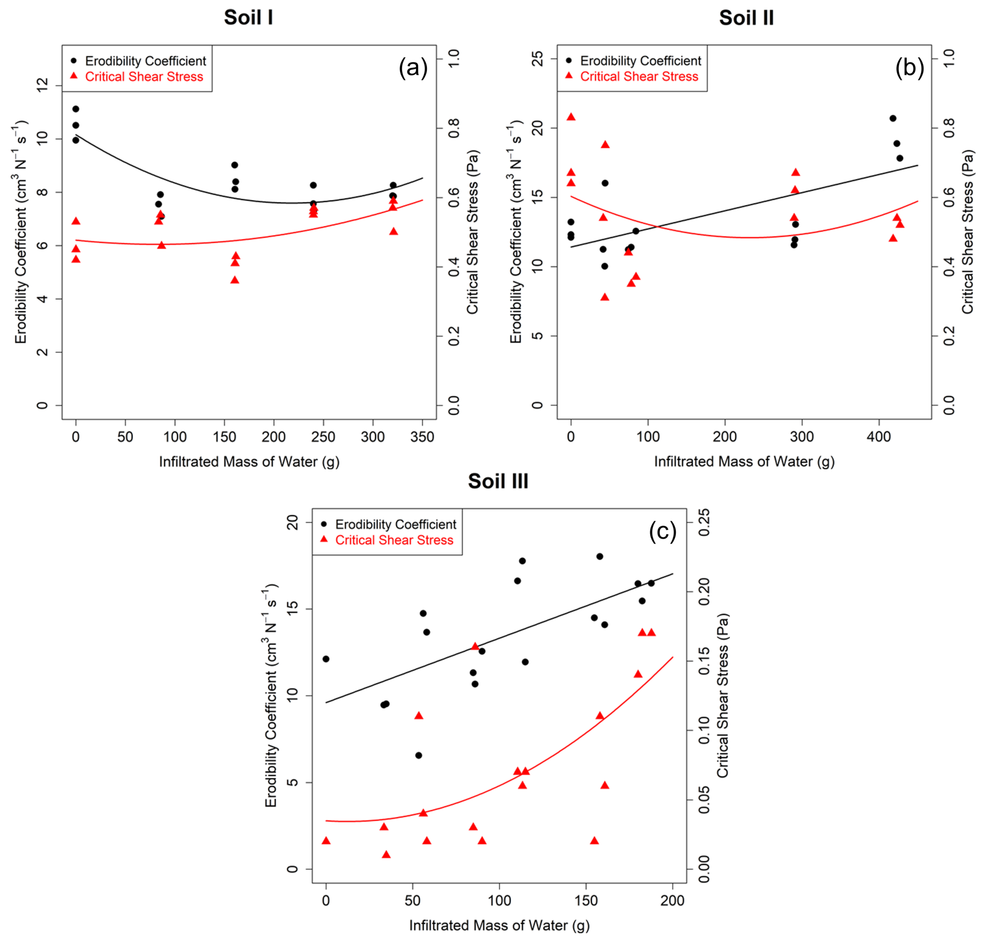
For each JET experiment, soil erodibility parameters ${\tau }_c$ and $k_d$ were derived with the Blaisdell solution using scour depth time series from Figure 4. Summary results of the soil erodibility parameters derived from 45 JET experiments are presented in Figure 5 for soils I, II, and III (Table 1). For each ${\tau }_c$ and $k_d$, a parabolic form regression fit Equation (8) was derived as a function of the mass of water:

$$P=b{M}^2+cM+d$$

(8)

where P is the erodibility parameter ($k_d$ or ${\tau }_c$), M is the mass of infiltrated water (g), and b, c, and d are constant regression coefficients. The calibrated values for b, c, and d and the coefficient of determination $R^2$ are shown separately for $k_d$ and ${\tau }_c$ in

Table 2. Average, dynamic, and baseline WEPP-based soil erodibility parameters $k_d$ (cm³N⁻¹s⁻¹) and ${\tau }_c$ (Pa) for soils I, II, and III. For the dynamic approach, the best-fit values of the coefficients b, c, d from Equation (8) are presented with the coefficient of determination $R^2$.

ID	Erodibility Coefficient						Critical Shear Stress
	Average  $\overline{{\mathit{k}}_{\mathit{d}}}$	Dynamic				WEPP  ${\mathit{k}}_{\mathit{d}}^{\mathit{WEPP}}$	Average  $\overline{{\mathbf{\tau }}_{\mathbf{c}}}$	Dynamic				WEPP  ${\mathit{\tau }}_{\mathit{c}}^{\mathit{WEPP}}$
		$\mathit{b}$	$\mathit{c}$	$\mathit{d}$	${\mathit{R}}^{\mathbf{2}}$			$\mathit{b}$	$\mathit{c}$	$\mathit{d}$	${\mathit{R}}^{\mathbf{2}}$
I	8.45	5.4 × 10−5	−2.35 × 10−2	10.2	0.63	4.83	0.5	1.79 × 10−6	−2.96 × 10−4	0.48	0.28	3.5
II	13.61	0	1.31 × 10−2	11.4	0.47	0.5	0.6	2.22 × 10−6	−1.03 × 10−3	0.60	0.07	1.4
III	13.44	0	3.72 × 10−2	9.6	0.45	13.11	0.1	3.36 × 10−6	−8.32 × 10−5	0.035	0.42	0.6

for each soil. The average $\overline{k_d}$ and $\overline{{\tau }_c}$ from all JET experiments are also shown in the table for each soil.

All soils showed significant changes in the derived erodibility coefficients over the range of tested masses of infiltrated water. Soil I displayed a curvelinear relationship for $k_d$, suggesting that there was an optimum time (210 g) during the infiltration process when it reached a minimum value. This observation follows similar trends in studies by Hanson and Hunt [24] and Hanson and Robinson [33], which concluded that there may be an optimum soil moisture content at which the erodibility coefficient is at a minimum. In contrast, soils II and III displayed almost a linear increase in $k_d$ with increasing infiltration which suggested that the soil detachment process would occur at a higher rate at later times during the infiltration process, assuming the applied hydraulic shear stress was higher than the critical shear stress during the process. Khanal et al. [23] observed similar increases in $k_d$ with increasing soil moisture content; however, they concluded that the trend observed for their sandy loam soil was statistically insignificant.

Critical shear stress displayed variability with increase of infiltrated mass of water. For soils I and II, ${\tau }_c$ displayed higher values for initially dry samples than for slightly infiltrated soils, with consecutive increases in ${\tau }_c$ with more water infiltrated into the sample (Figure 5a,b). Soil III displayed a positive curvelinear relationship with the values increasing an order of magnitude from 0.012 Pa for M < 100 g to 0.16 Pa for M close to 180 g (Figure 5c). These results suggest that when water infiltrates into the soil profile, clay loam soils I and II are likely more susceptible to erosion than sandy loam soil III during smaller runoff or other events where the applied hydraulic shear stress is low, while sandy loam soil III can be more resistant to erosion as the infiltration process progresses and soil becomes saturated.

4. Discussion

The results from the mini-JETs showed the variability in estimated erodibility coefficients with the values reflecting the change in initial soil moisture condition and amounts of infiltrated water M. The critical shear stress exhibited a decrease with the increase of M, while the erodibility coefficient generally showed an increase for soils II and III with slightly higher values at $M=0$ g for soil I (Figure 5). The variability in parameters was indicative of the variability in scour depth curves in Figure 4. The increase of M generally produced deeper scours immediately from the beginning of each JET test. Higher initial scours for relatively dry soils I and II resulted in higher ${\tau }_c$ values for lower M. The scour growth rate was significantly higher for sandy loam soil III than for (silty) clay loam soils I and II at any M due to higher sand content and higher soil bulk density (see Table 1).

For comparison with the experiments, the WEPP-based baseline constants $k_d$ and ${\tau }_c$ are presented for the three studied soils in Table 2. Based on the baseline conditions alone, the JET-averaged values $\overline{k_d}$ and $\overline{{\tau }_c}$ were different from the WEPP-based baseline $k_d^{WEPP}$ and ${\tau }_c^{WEPP}$ values for soils I and II, while soil erodibility coefficient values were close for soil III.

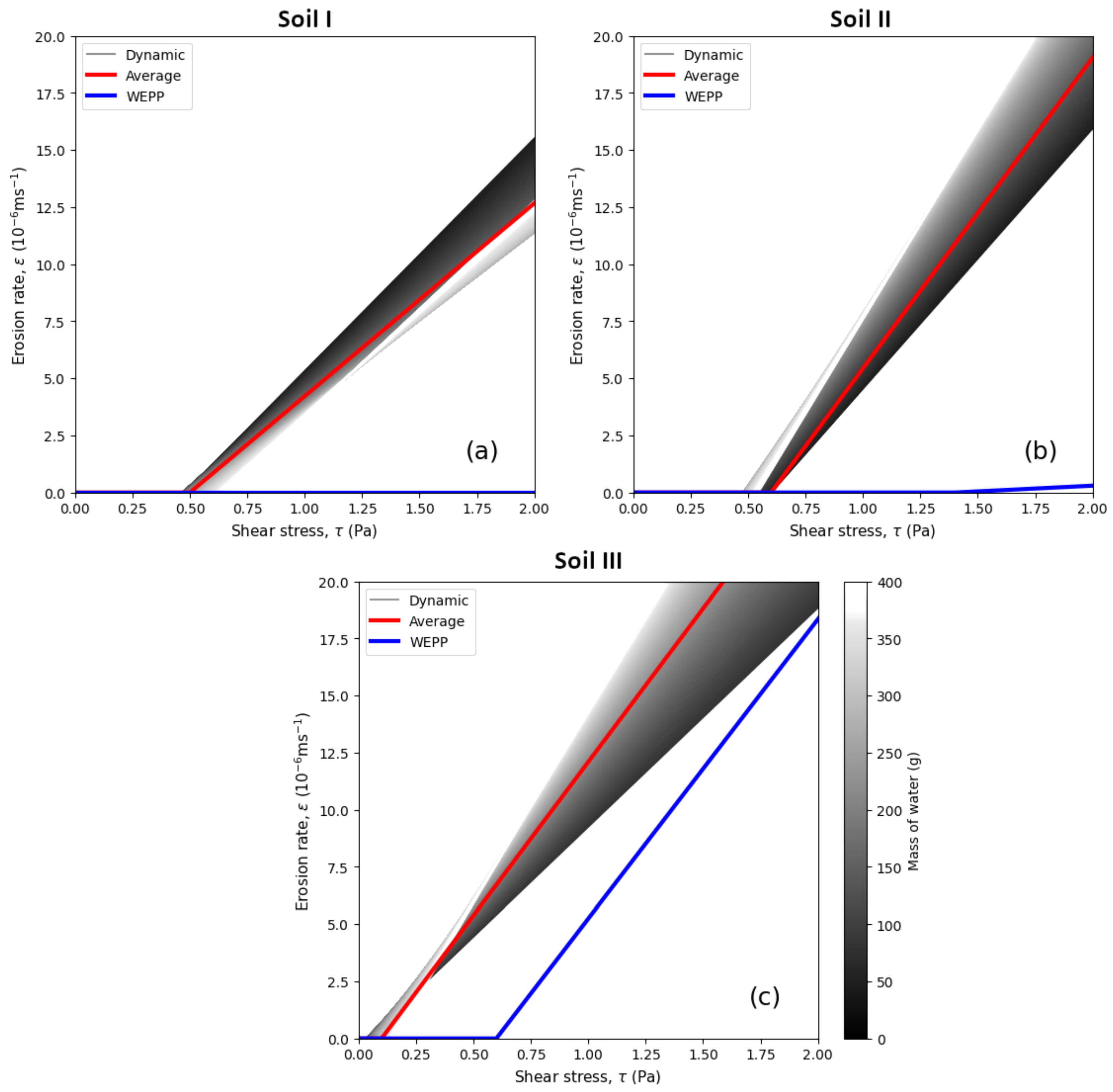
To quantify the effect of the dynamic nature of soil erodibility parameters observed in the JET experiments on the prediction of soil erosion, the erosion rates $\epsilon$ in Equation (1) were calculated for each soil using three approaches for the estimation of the erodibility parameters (Table 2). The values of $k_d$ and ${\tau }_c$ were evaluated as follows:

(i)

Dynamic $k_d$ and ${\tau }_c$ as a function of mass of infiltrated water M with coefficients b, c, and d;

(ii)

Average values $\overline{k_d}$ and $\overline{{\tau }_c}$, and;

(iii)

Baseline coefficients $k_d^{WEPP}$ and ${\tau }_c^{WEPP}$ from the WEPP model.

In approach (i), the erosion rate $\epsilon$ changes based on the values of $k_d$ and ${\tau }_c$ adjusted for the amount of infiltrated water M, while approaches (ii) and (iii) utilize constant coefficients. The erosion rate is calculated as a function of hydraulic shear stress $\tau$ and presented in Figure 6 for different approaches. The erosion rate is zero for $\tau <{\tau }_c$ and linearly increases afterwards. The dynamic erosion rates for approach (i) are presented as a grayed area to visualize how the range of infiltrated mass of water M varied from 0 g (light gray) to up to 400 g (dark gray). The range of the erosion rate widens with the increase of $\tau$. Since ${\tau }_c^{WEPP}$ are greater than the dynamic and average ${\tau }_c$, the erosion rate for JET-derived coefficients starts at lower values of $\tau$ (gray and red curves) and exceeds WEPP estimated values of $\epsilon$. For higher $\tau >2$ Pa for soil III, the dynamic range of $\epsilon$ can encapsulate the estimates from both (ii) average and (iii) WEPP approaches.

During a surface runoff event, rate of overland flow and hydraulic shear stresses applied at soil surface can vary with time and event intensity, thus causing variable soil detachment and subsequently soil erosion rates [22]. At the same time, surface water infiltrated into soil can affect soil cohesiveness and cause pore pressure to rise. The effect can differ for soils of different texture, plasticity, and cohesiveness. The magnitude of that effect and its impact on soil detachment and soil erosion are not well understood.

In regards to the formulation in Equation (1), the infiltrated water during the rainfall event makes soil moisture content time-dependent, which dynamically affects both erodibility parameters $k_d$ and ${\tau }_c$ according to Figure 5. In response, the corresponding effect on soil erosion rates can vary, with a higher range of variability for higher runoff depths (see Figure 6). This experimental study presents an attempt to quantify the combined effect of water infiltration and applied shear stresses on soil erodibility. Although the erodibility coefficients $k_d$ and ${\tau }_c$ were found to be dependent on the infiltrated mass of water, the impact is distinctive but relatively mild, especially at the lower $\tau$, and needs additional assessment with JET or other laboratory and field experiments.

5. Conclusions

The effects of infiltration and soil water content on soil erodibility parameters were analyzed for three soils (clay loam, silty clay loam, and sandy loam) using the laboratory Jet Erosion Test. Soil samples were prepared and subjected to infiltration with different masses of infiltrated water prior to each JET. Scour depths were recorded for 45 JET experiments and analyzed with the Blaisdell solution for the erodibility parameters $k_d$ and ${\tau }_c$. Results from these experiments not only showed variability in the erodibility parameters across different soil types but also depicted a dynamic relationship between the soil erodibility parameters and mass of infiltrated water.

To determine the impact of the dynamic nature of the derived soil erodibility parameters on soil erosion, the erosion rates were calculated with an excess shear stress equation for three studied soils over a broad range of applied hydraulic shear stresses $\tau$ using three different approaches. The approaches included determining the parameters as a function of infiltrated mass of water, using average values from this study, or applying specific formulas from the Water Erosion Prediction Project (WEPP) model. The WEPP approach produced lower erosion rates compared to both the dynamic and average approaches, mainly due to higher values of the estimated critical shear stress. We note that WEPP-based erodibility approach represents baseline soil condition and does not account for soil specific features, such as, residue, plant roots and biomass, and soil crusting and sealing. The impact of dynamic erodibility parameters is seen at any applied shear stress but the estimated erosion rates have a wider range of values for higher $\tau$.

The results of this study highlight the importance of evaluating the effects that soil moisture or water infiltration rates during surface runoff events have on soil erosion. Specifically, a concave form of the critical shear stress curve may impact the threshold for the acting shear stress to initiate soil particle detachment at low antecedent soil moisture condition. The increase in erodibility coefficient with soil moisture content can enhance soil erosion rates once the soil becomes more saturated during the rainfall event. As the direct impact of infiltrated mass of water or soil moisture on the erodibility parameters is difficult to evaluate in situ, the use of proxy factors can be considered, such as antecedent soil moisture content, time to peak from the start of runoff, soil cohesion, etc. Further assessment of such factors with JET or other laboratory and field tests is recommended.

References

1. Nusser, S.M.; Goebel, J.J. The National Resources Inventory: A long-term multi-resource monitoring programme. Environ. Ecol. Stat. 1997, 4, 181–204. [Google Scholar] [CrossRef]
2. Huffman, R.; Fangmeier, D.; Elliot, W.; Workman, S. Soil and Water Conservation Engineering; American Society of Agricultural and Biological Engineers (ASABE) Publication: St. Joseph, MI, USA, 2013. [Google Scholar]
3. Fox, G.A.; Sheshukov, A.; Cruse, R.; Kolar, R.L.; Guertault, L.; Gesch, K.R.; Dutnell, R.C. Reservoir Sedimentation and Upstream Sediment Sources: Perspectives and Future Research Needs on Streambank and Gully Erosion. Environ. Manag. 2016, 57, 945–955. [Google Scholar] [CrossRef] [PubMed]
4. Partheniades, E. Erosion and Deposition of Cohesive Soils. J. Hydraul. Div. 1965, 91, 105–139. [Google Scholar] [CrossRef]
5. Knapen, A.; Poesen, J.; Govers, G.; Gyssels, G.; Nachtergaele, J. Resistance of soils to concentrated flow erosion: A review. Earth-Sci. Rev. 2007, 80, 75–109. [Google Scholar] [CrossRef]
6. Hanson, G.J.; Cook, K.R. Apparatus, Test Procedures, and Analytical Methods to Measure Soil Erodibility in Situ. Appl. Eng. Agric. 2004, 20, 455–462. [Google Scholar] [CrossRef]
7. USDA-ARS. USLE History. 2016. Available online: https://www.ars.usda.gov/midwest-area/west-lafayette-in/national-soil-erosion-research/docs/usle-database/usle-history/ (accessed on 10 November 2023).
8. Leopold, L.B.; Emmett, W.W.; Myrick, R.M. Channel and Hillslope Processes in a Semiarid Area, New Mexico; U.S. Government Printing Office: Washington, DC, USA, 1966. [CrossRef]
9. Hanson, G.J.; Cook, K.R. Development of Excess Shear Stress Parameters for Circular Jet Testing; ASAE Paper 972227; ASABE: St. Joseph, MI, USA, 1997. [Google Scholar]
10. Al-Madhhachi, A.T.; Hanson, G.J.; Fox, G.A.; Tyagi, A.K.; Bulut, R. Measuring Soil Erodibility Using a Laboratory “Mini” Jet. Trans. ASABE 2013, 56, 901–910. [Google Scholar] [CrossRef]
11. Daly, E.R.; Fox, G.A.; Al-Madhhachi, A.T.; Miller, R.B. A Scour Depth Approach for Deriving Erodibility Parameters from Jet Erosion Tests. Trans. ASABE 2013, 56, 1343–1351. [Google Scholar] [CrossRef]
12. Blaisdell, F.W.; Hebaus, G.G.; Anderson, C.L. Ultimate Dimensions of Local Scour. J. Hydraul. Div. 1981, 107, 327–337. [Google Scholar] [CrossRef]
13. Liu, Q.; Wells, R.; Dabney, S.; He, J. Effect of Water Potential and Void Ratio on Erodibility for Agricultural Soils. Soil Sci. Soc. Am. J. 2017, 81, 622–632. [Google Scholar] [CrossRef]
14. Khanal, A.; Fox, G.A.; Al-Madhhachi, A.T. Variability of Erodibility Parameters from Laboratory Mini Jet Erosion Tests. J. Hydrol. Eng. 2016, 21, 04016030. [Google Scholar] [CrossRef]
15. Flanagan, D.C.; Ascough, J.C.; Nicks, A.D.; Nearing, M.A.; Laflen, J.M. Chapter 1. Overview of the WEPP Erosion Prediction Model. In USDA-Water Erosion Prediction Project (WEPP); NSERL: West Lafayette, IN, USA, 1995; pp. 1.1–1.12. Available online: https://www.ars.usda.gov/midwest-area/west-lafayette-in/national-soil-erosion-research/docs/wepp/wepp-model-documentation/ (accessed on 1 March 2024).
16. Alberts, E.E.; Nearing, M.A.; Weltz, M.A.; Risse, L.M.; Pierson, F.B.; Zhang, X.C.; Laflen, J.M.; Simanton, J.R. Chapter 7. Soil Component. In USDA-Water Erosion Prediction Project (WEPP); NSERL: West Lafayette, IN, USA, 1995; pp. 7.1–7.47. Available online: https://www.ars.usda.gov/midwest-area/west-lafayette-in/national-soil-erosion-research/docs/wepp/wepp-model-documentation/ (accessed on 1 March 2024).
17. Lisenbee, W.A.; Fox, G.A.; Saenz, A.; Miller, R.B. Comparison of Field Jet Erosion Tests and WEPP-Predicted Erodibility Parameters for Varying Land Cover. Trans. ASABE 2017, 60, 173–184. [Google Scholar] [CrossRef]
18. Potter, K.N.; Velazquez-Garcia, J.d.J.; Torbert, H.A. Use of a Submerged Jet Device to Determine Channel Erodibility Coefficients of Selected Soils of Mexico. J. Soil Water Conserv. 2002, 57, 272–277. [Google Scholar]
19. Nouwakpo, S.K.; Huang, C.-h.; Bowling, L.; Owens, P. Impact of Vertical Hydraulic Gradient on Rill Erodibility and Critical Shear Stress. Soil Sci. Soc. Am. J. 2010, 74, 1914. [Google Scholar] [CrossRef]
20. Al-Madhhachi, A.T.; Fox, G.A.; Hanson, G.J.; Tyagi, A.K.; Bulut, R. Mechanistic Detachment Rate Model to Predict Soil Erodibility Due to Fluvial and Seepage Forces. J. Hydraul. Eng. 2014, 140, 04014010. [Google Scholar] [CrossRef]
21. Karimov, V.; Sheshukov, A.Y.; Barnes, P. Impact of precipitation and runoff on ephemeral gully development in cultivated croplands. In Sediment Dynamics: From the Summit to the Sea; Xu, Y.J., Ed.; IAHS Publ. 367; IAHS Press: Wallingford, UK, 2015; pp. 87–92. [Google Scholar] [CrossRef]
22. Karimov, V.; Sheshukov, A.Y. Effects of Intra-Storm Soil Moisture and Runoff Characteristics on Ephemeral Gully Development: Evidence from a No-Till Field Study. Water 2017, 9, 742. [Google Scholar] [CrossRef]
23. Khanal, A.; Fox, G.A.; Guertault, L. Soil Moisture Impacts Linear and Nonlinear Erodibility Parameters from Jet Erosion Tests. Trans. ASABE 2020, 63, 1123–1131. [Google Scholar] [CrossRef]
24. Hanson, G.J.; Hunt, S.L. Lessons Learned using Laboratory JET Method to Measure Soil Erodibility of Compacted Soils. Appl. Eng. Agric. 2007, 23, 305–312. [Google Scholar] [CrossRef]
25. Graf, W.H. Cohesive-material channels. In Hydraulics of Sediment Transport, 3rd ed.; Water Resources Publications: Brookvale, Australia, 1984; pp. 335–337. [Google Scholar]
26. Huang, C.; Laften, J.M. Seepage and Soil Erosion for a Clay Loam Soil. Soil Sci. Soc. Am. J. 1996, 60, 408–416. [Google Scholar] [CrossRef]
27. Nachtergaele, J.; Poesen, J. Spatial and temporal variations in resistance of loess-derived soils to ephemeral gully erosion. Eur. J. Soil Sci. 2002, 53, 449–463. [Google Scholar] [CrossRef]
28. Nguyen, G.H.T. Evaluating Soil Erodibility Parameters with Mini-Jet Under Various Soil Moisture Conditions. Master’s Thesis, Kansas State University, Manhattan, KS, USA, 2016. [Google Scholar]
29. Akin, A.A.; Sheshukov, A.Y. Soil erodibility parameters for two soils with different soil moisture content evaluated with the mini-Jet Erosion Test (JET). Mendeley Data. 2024. Available online: https://data.mendeley.com/datasets/c28fnf34pk/1 (accessed on 1 March 2024). [CrossRef]
30. Soil Science Division Staff. Soil Science Division Staff. Soil survey manual. In USDA Handbook 18; Ditzler, C., Scheffe, K., Monger, H.C., Eds.; Government Printing Office: Washington, DC, USA, 2017. [Google Scholar]
31. Kansas State University, Department of Agronomy. K-State Soil Testing Lab. 2021. Available online: https://www.agronomy.k-state.edu/outreach-and-services/soil-testing-lab/ (accessed on 1 March 2024).
32. ASTM D698; Standard Test Methods for Laboratory Compaction Characteristics of Soil Using Standard Effort (12,400 ft-lbf/ft3 (600 kN-m/m3)). American Society for Testing and Materials: West Conshohocken, PA, USA, 2012.
33. Hanson, G.J.; Robinson, K.M. The Influence of Soil Moisture and Compaction on Spillway Erosion. Trans. ASAE 1993, 36, 1349–1352. [Google Scholar] [CrossRef]
Figure 1. Soil sample before and after the infiltration experiment: (a) standard mold filled with compacted soil, (b) soil specimen after soil core extraction, and (c) soil moisture in a core after the infiltration experiment.
Water 16 00981 g001
Figure 2. Laboratory setup for (a) infiltration test and (b) JET erosion experiment.
Water 16 00981 g002
Figure 3. Average soil moisture profiles with depth at each tested infiltrated mass of water for (a) soil I, (b) soil II, and (c) soil III.
Water 16 00981 g003
Figure 4. Scour depth with time for JET experiments for three soils: (a) soil I, (b) soil II, and (c) soil III. Open circles represent scour depth readings for each JET experiment, and solid curves show best-fit lines for each group of mass of infiltrated water.
Water 16 00981 g004
Figure 5. Soil erodibility parameters ( k d and τ c ) versus mass of infiltrated water derived from JET experiments for three tested soils: (a) soil I, (b) soil II, and (c) soil III.
Water 16 00981 g005
Figure 6. Soil erosion rates ε versus hydraulic shear stress τ calculated with Equation (1) and erodibility parameters k d and τ c using three approaches: (i) dynamic as function of mass M of infiltrated water (gray band), (ii) average from JET experiments (red line), and (iii) WEPP-based (blue line), for three soils: (a) soil I, (b) soil II, and (c) soil III. The ranges of k d and τ c values for the dynamic approach were exported from Equation (8) with the coefficients b, c, and d from Table 2.
Water 16 00981 g006