Post-Analysis of Daniel Extreme Flood Event in Thessaly, Central Greece: Practical Lessons and the Value of State-of-the-Art Water-Monitoring Networks

Abstract

Storm Daniel initiated on 3 September 2023, over the Northeastern Aegean Sea, causing extreme rainfall levels for the following four days, reaching an average of about 360 mm over the Peneus basin, in Thessaly, Central Greece. This event led to extensive floods, with 17 human lives lost and devastating environmental and economic impacts. The automatic water-monitoring network of the HIMIOFoTS National Research Infrastructure captured the evolution of the phenomenon and the relevant hydrometeorological (rainfall, water stage, and discharge) measurements were used to analyse the event’s characteristics. The results indicate that the average rainfall’s return period was up to 150 years, the peak flow close to the river mouth reached approximately 1950 m³/s, and the outflow volume of water to the sea was 1670 hm³. The analysis of the observed hydrographs across Peneus also provided useful lessons from the flood-engineering perspective regarding key modelling assumptions and the role of upstream retentions. Therefore, extending and supporting the operation of the HIMIOFoTS infrastructure is crucial to assist responsible authorities and local communities in reducing potential damages and increasing the socioeconomic resilience to natural disasters, as well as to improve the existing knowledge with respect to extreme flood-simulation approaches.

1. Introduction

Floods are among the most destructive natural hazards, with dramatic human and economic impacts at the global scale [1,2,3,4,5,6,7,8]. Floods can be classified as fluvial (i.e., due to river overflows), pluvial, flash floods, coastal floods, and floods induced by infrastructure failure, such as levee or dam breaches [9,10]. Factors such as the increase in population density close to rivers (i.e., the decrease of the human–flood distance) [11], fast economic growth in river plains, and changes in land uses tend to further compound the disastrous effects of floods, putting at even higher risk flood-prone areas and, thus, posing a major threat to human life, properties, and infrastructures [12,13,14,15,16]. Moreover, floods can harm the entire spectrum of productive activities, strongly impacting agricultural production, raising food prices, and causing adverse effects on tourism and the local economy [17].

Within an integrated flood-protection framework, managing the flood risk and mitigating the adverse consequences related to floods, requires the co-implementation of both structural and non-structural measures [18,19]. With respect to the non-structural approaches, which are also highly promoted by the current legislation framework (e.g., the Floods Directive 2007/60/EC), real-time flood forecasting and early-warning systems are considered among the most effective measures to minimize casualties and reduce damages [20]. This is typically achieved through the timely dissemination of flood-risk-related information, often in the form of flood-risk and hazard maps or estimated flood travel times, which facilitate the early evacuation of cities and villages [18,21].

Flood forecasting and early-warning systems most often rely on computer models (mostly conceptual, with some physical basis) simulating the hydrological processes and flow routing dynamics or on rather black-box (e.g., stochastic, computational intelligent) techniques, relating precipitation and/or upstream stage/discharge data with the river’s response or combinations thereof [22,23]. In all approaches, the availability of adequate in situ observations is indispensable, to calibrate/validate the associated models, thus extracting reliable and robust predictions [24].

Although more detailed simulators are generally considered more accurate in the prediction of inundation extent and water depths, they are “data-intensive” and demanding in terms of accuracy and spatial distribution of the required data. Most importantly, though, they demand increased computational resources, especially in the case of 2D hydrodynamic approaches, where run times may be on the order of hours or days, depending on the extent and resolution of the computational grid [25]. This often renders them impractical for operational forecasting systems, where achieving short prediction times is crucial [26]. In this regard, in flood forecasting approaches, there is a recent tendency towards “parsimony”, that is lower-fidelity hydrodynamic models, as surrogates of more detailed ones, or data-driven approaches by means of machine-learning techniques [27,28,29,30,31,32,33,34].

Acknowledging that simplified approaches are preferable in cases where a timely but still reliable warning is of high priority, flood travel time and flood celerity have been widely recognized as key informative metrics for alert and forecasting purposes [3,35,36,37,38], as well as for decision-making and optimization of flood-management structures [39,40,41]. The first typically refers to the time required for a flood-wave crest to move from an upstream to a downstream location along a given reach [42], while both variables can be theoretically extracted through hydrodynamic modelling approaches (e.g., [3,36,37,42,43]). In practice, flood-wave celerity can also be empirically estimated at the “reach scale” by dividing the distance between two monitoring stations by the measured travel time. Several studies have exploited in situ streamflow observations to estimate celerity in rivers and identify patterns depending on the flow and river characteristics (e.g., [41,44]).

In order to reveal the major role of flow-monitoring data as a means to improve our knowledge of large-scale floods and provide decision support in the context of flood-management practices, we employ a post-analysis of the recent catastrophic flood event caused by the tropical-like cyclone “Daniel” over the Thessaly Region. The greatest part of Thessaly falls into the Peneus river basin, which drains a total area of 11,063 km². Storm Daniel occurred between 3 and 8 September 2023 and also hit extended parts of the Mediterranean region. This phenomenon was characterized as the most intense and costly recorded storm event for the country in the 21st century, inducing extensive and irreparable damages.

The evolution of this catastrophic event, with respect to the hydrological response of the river basin, was captured by seven automatic hydrometric stations, operating under the coordination of the Hellenic Centre for Marine Research (HCMR) (https://imbriw.hcmr.gr/, accessed on 15 February 2023) and developed in the framework of a National Research Infrastructure project (see Section 2.1.3). In Greece, water-monitoring networks that provide systematic data in real time are extremely rare, except for a few sparse and isolated efforts, operating on limited spatial and temporal scales. Hence, the objective of this work is to utilize the raw hydrometric information (i.e., river stage data) in order to: (a) implement a post-analysis of the magnitude and main features of the event; (b) enrich our knowledge of large flood events across large-scale basins and get lessons for engineering practice, and (c) investigate the potential of the existing monitoring network to act as a fast and cost-effective tool towards flood forecasting and early warning. For this purpose, we also took advantage of two other sources of easily retrievable data, namely precipitation data from a large number of meteorological stations in the broader area of interest and satellite maps of inundated areas in an effort to analyse this extreme event and, thus, gain insights in the hydrological response of the watershed to low-frequency storms. Additionally, the flood travel time along the river was estimated for Storm Daniel and for selected past events of high magnitude.

2. Materials and Methods

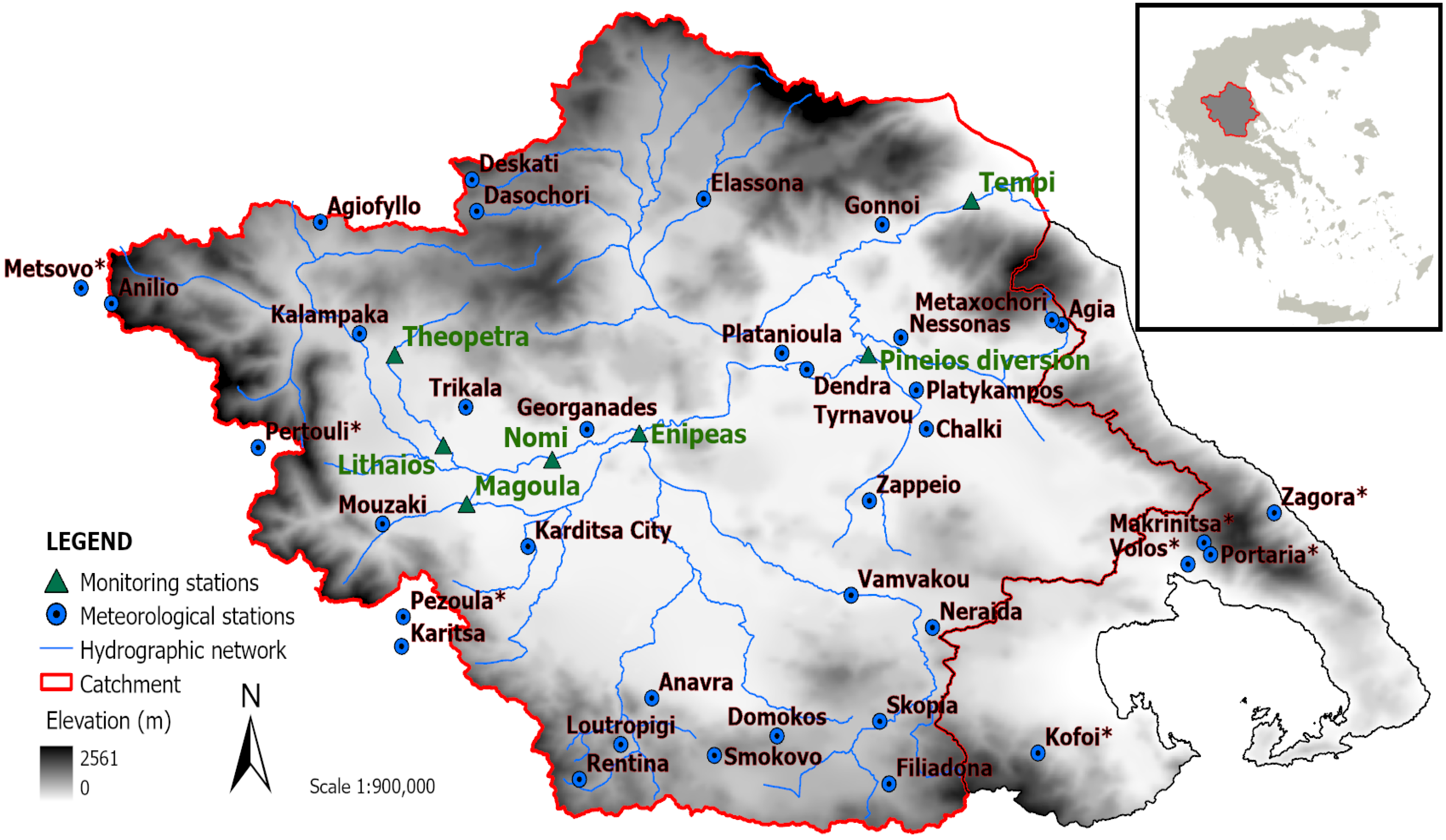
2.1. Study Area

2.1.1. Geomorphology and Climate

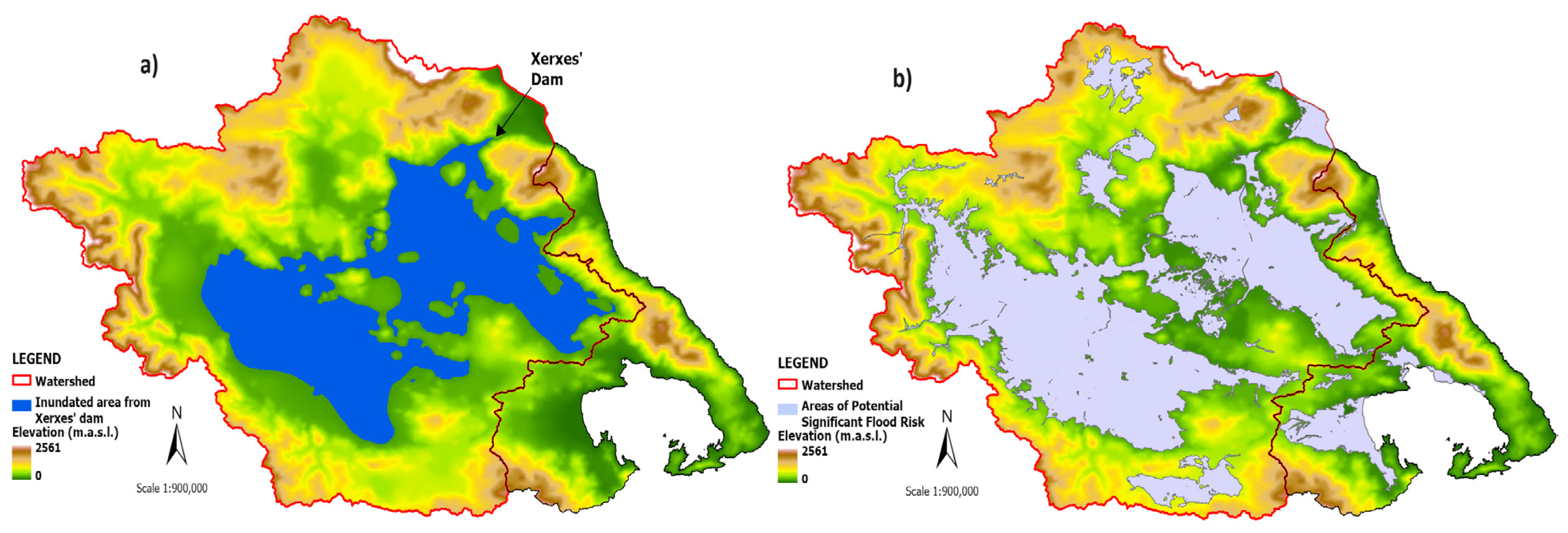
The Peneus river basin (Figure 1), located in Thessaly, Central Greece, from 39°11′ to 39°58′ N and 21°52′ to 22°45′ E, covers a total area of about 11,063 km². The minimum, maximum, and mean elevations of the basin are 0, 2085, and 440 m, respectively. Peneus is the third-longest river in Greece, with a total length of about 260 km. It springs from the Pindus mountains and consists of an extended river network of about 1200 km. After crossing the narrow valley of Tempi, the river empties into the Aegean Sea [45].

The lower parts of the study area are mainly characterized by flat terrain and are covered by the Thessaly Plain, which is among the most intensively cultivated areas and the second most productive agricultural area in Greece [45,46]. Cotton, winter wheat, maize, and alfalfa are some of the main crops cultivated in the plain [47], while agriculture constitutes the dominant land use in the area; along with pasture, they cumulatively correspond to about half of the catchment’s total extent.

The coastal part of the watershed has a typical Mediterranean climate, while the western and central areas have a continental climate, characterized by hot summers and cold winters. The rainfall varies considerably across the watershed, from about 360 mm annually in the central and coastal areas to about 1850 mm in the mountainous part; the mean annual precipitation, considering the entire basin, has been estimated at about 780 mm [48]. The flow regime of the Peneus River is characterized as perennial, with a marked discharge variation across seasons. In particular, the mean monthly streamflow near Peneus’ Delta lies in the range of 150 m³/s (annual average for February and March) to 10 m³/s (annual average for August and September), with a mean annual value of about 80 m³/s [48].

2.1.2. Flood Regime

As shown in Figure 1, the morphology of Thessaly comprises extended low areas enclosed by high mountains that receive large amounts of rainfall. This landscape resembles a lake, draining through a narrow valley in the east. As a result, significant parts of the basin, corresponding approximately to 36.7% of its total extent, have been identified as Areas with Potential Significant Flood Risk (APSFR; Figure 2b), according to the Flood Directive 2007/60/EC [49].

In fact, the lower parts of Thessaly lie on a paleolake, the existence of which is dated to several thousand years ago and is also mentioned by the Greek historian Herodotus (who lived during the 5th century BC) in his book Histories (7.129). Herodotus also reveals the exposure of Thessaly to floods in the following quotation (Histories, 7.130.1-2; translation) [50]:

“Xerxes asked his guides if there were any other outlet for the Peneus into the sea, and they, with their full knowledge of the matter, answered him: “The river, O king, has no other way into the sea, but this alone. This is so because there is a ring of mountains around the whole of Thessaly”. Upon hearing this Xerxes said: “These Thessalians are wise men; this, then, was the primary reason for their precaution long before when they changed to a better mind, for they perceived that their country would be easily and speedily conquerable. It would only have been necessary to let the river out over their land by barring the channel with a dam and to turn it from its present bed so that the whole of Thessaly, with the exception of the mountains, might be under water”.

The Persian ruler Xerxes passed from the area during his invasion of Greece in the years 480–479 BC. According to the above quotation, Xerxes explained the compliance of Thessalians to his rule by the threat of constructing a dam at the mouth of Peneus. Representing Xerxes’ threat, we consider a hypothetical dam of 100 m in height and map the derived reservoir extent through GIS techniques (Figure 2a). By contrasting the virtual reservoir with the APSFRs (Figure 2b), an impressive resemblance emerges, which explains the significant vulnerability of Thessaly against floods.

It is known that the Thessaly Plain has suffered from floods since antiquity, while extended areas were covered by wetlands and marshes up to the beginning of the 20th century, also causing fatalities due to malaria. In this vein, the Greek state commissioned the USA company BOOT to furnish Thessaly with large-scale flood-protection infrastructures. The land reclamation works started in 1934 and were completed in 1961 with the draining of Lake Karla. These works allowed for the release of extended areas of high fertility, while radically improving the health conditions and the quality of life of inhabitants [51]. Subsequently, further improvements were made through the development of drains and irrigation networks, the restoration of Lake Karla, and the construction of the Smokovo dam, which has contained all floods produced in the upstream basin since 2002 (which, however, covers a very small proportion of the entire basin, i.e., 376 km²). Today, there is an extensive network of regulated streams, collectors, and drainage ditches, while levees have been constructed along many lowland streams, creating controlled basins.

Despite the implementation of several streamlining works and land reclamation projects until the early 20th century, the Peneus River still experiences floods quite often. In particular, 22 severe floods have been reported since 1979 [49]. The main causes of flooding in the lowlands of Thessaly are (1) the existence of several closed basins requiring pumping for their drainage, (2) the limited discharge capacity across extended parts of the channel network, also due to vegetation and sediment deposits, (3) the insufficient openings of bridges and culverts, (4) the damages of levees and malfunction of control gates during severe floods, resulting in significant overflows, (5) the construction of temporary irrigation dams along riverbeds, and (6) the acceleration of the flood runoff of the mountain basins due to drainage works and land-use changes.

2.1.3. Hydrometric Network

The hydrometric monitoring stations that are exploited in the present work are located along the main course of Peneus and its major tributaries (Figure 1), and they are part of the national-scale network of the HCMR, Department of Inland Water. The first ones were installed within the development of the research infrastructure “Hellenic Integrated Marine Inland water Observing Forecasting and offshore Technology System” (HIMIOFoTS; https://www.himiofots.gr/, accessed on 27 September 2023), particularly its freshwater component (https://openhi.net/en/) [52], and the rest under the project Open ELIoT (https://www.openeliot.com/, accessed on 27 September 2023).

The hydrometric network comprises seven automatic monitoring stations, providing real-time measurements of water level and selected water-quality parameters on hourly or 30 min time steps. The first station (Nomi) was established in August 2019. At most locations, discharge time series were estimated either through stage–discharge curves or based on surface flow-velocity measurements using radar sensors (Geolux RSS-2-300WL, https://www.geolux-radars.com/rss2300wl, accessed on 27 November 2023, Geolux company, Zagreb, Croatia). The recorded measurements of all telemetric stations are automatically stored on an FTP server and are available online on a near real-time basis. In the current analysis, six monitoring sites were considered to describe the evolution of the flood event, among which three (Tempi, Peneus diversion, and Nomi) are located on the main river course and three on its tributaries (Enipeas, Magoula, and Theopetra). The main characteristics of the hydrometric stations are provided in

Table 1. Main characteristics of monitoring sites and measurements considered (all stations have water-level and discharge measurements, apart from the Peneus diversion, which has only water level).

Monitoring Station	Lat. (°)	Lon. (°)	Elev. (m)	Upstream Area (km2)	Discharge Estimation	Time Step
Tempi	39.8968	22.6152	3.5	10,591	Velocity	30 min
Peneus diversion	39.6525	22.4078	61.9	6544	-	30 min
Nomi	39.5266	21.9383	91.2	2243	Velocity	30 min
Magoula	39.4634	21.7995	106.0	222	Stage–discharge curve	1 h
Enipeas	39.5635	22.0802	86.1	2640	Stage–discharge curve	30 min
Theopetra	39.6748	21.6788	173.0	118	Stage–discharge curve	1 h

.

2.1.4. Rainfall Analysis

Overall, 38 meteorological stations are considered, which are shown in Figure 1 (30 lie within the river-basin boundaries, while 10 are peripheral). One station (Georganades) belongs to the HCMR, Department of Inland Water, two stations (Filiadona and Metaxochori) are part of the Weather Underground (WU) network (https://www.wunderground.com/), eight belong to the Ministry of Environment and Energy (MinEnv), whereas the remaining rainfall data were retrieved from the “meteo” site of the National Observatory of Athens (NOA; https://www.meteo.gr/). For Filiadona, Georganades, Metaxochori, and Pertouli, we gained rainfall records at fine temporal resolution, while for the rest only their daily values were freely available. The station characteristics and rainfall depths during the four-day storm period (from 4 to 7 September 2023) are shown in

Table 2. Meteorological stations over the broader area of interest and daily rainfall values during the evolution of Storm Daniel (from 4 to 7 September 2023). Peripheral stations are denoted with (*).

Station	$\mathit{X}$ (m)	$\mathit{Y}$ (m)	$\mathit{Z}$ (m)	Owner	Daily Rainfall Values (mm)				Total (mm)
					4/9	5/9	6/9	7/9
Agia	393,482	4,396,908	200.0	NOA	11.2	218.6	15.4	90.6	335.8
Agiofyllo	291,669	4,415,392	584.1	MinEnv	60.0	40.0	54.0	-	154.5
Anavra	335,689	4,338,439	196.3	MinEnv	98.0	131.0	218.0	0.0	447.0
Anilio	262,521	4,403,261	1660.0	NOA	20.6	148.2	374.6	149.2	692.6
Chalki	374,539	4,380,625	75.0	NOA	25.2	180.8	68.8	30.4	305.2
Dasochori	313,228	4,416,564	737.0	NOA	13.8	98.6	46.4	23.0	181.8
Dendra Tyrnavou	358,191	4,390,372	75.0	NOA	19.2	86.4	64.8	22.8	193.2
Deskati	312,700	4,421,617	769.0	NOA	10.4	96.0	50.6	25.6	182.6
Domokos	352,968	4,332,057	570.0	NOA	40.4	110.0	225.2	6.4	382.0
Elassona	344,494	4,417,838	282.0	NOA	26.4	72.2	19.6	40.8	159.0
Filiadona	368,423	4,324,135	487.0	WU	23.1	72.5	125.5	9.1	230.2
Georganades	327,623	4,381,444	92.0	HCMR	24.8	116.3	195.8	28.9	365.8
Gonnoi	368,984	4,413,284	111.0	NOA	14.0	147.4	31.4	71.2	264.0
Kalampaka	296,582	4,397,471	238.0	NOA	10.8	94.2	165.8	85.2	356.0
Karditsa City	319,027	4,362,984	121.0	NOA	42.4	185.2	404.4	26.8	658.8
Karitsa	301,118	4,347,487	1074.3	MinEnv	90.0	110.0	110.0	300.0	610.0
Kofoi *	389,232	4,328,735	500.0	NOA	23.4	152.6	342.2	32.2	550.4
Loutropigi	331,211	4,331,131	722.1	MinEnv	0.0	98.5	86.5	99.6	284.6
Makrinitsa *	412,701	4,361,962	850.0	NOA	125.2	757.4	273.6	79.2	1235.4
Makrinitsa *	412,260	4,361,258	685.4	MinEnv	75.0	82.0	-	38.4	-
Metaxochori	392,122	4,397,704	340.0	WU	14.0	170.7	14.7	60.7	260.1
Metsovo *	258,410	4,405,870	1240.0	NOA	20.2	91.8	204.0	75.8	391.8
Mouzaki	298,972	4,367,063	175.0	NOA	23.8	163.8	321.8	89.0	598.4
Neraida	374,872	4,348,963	243.0	NOA	19.6	226.6	91.2	23.8	361.2
Nessonas	371,249	4,395,250	92.0	NOA	11.6	78.0	3.6	71.6	164.8
Pertouli *	282,096	4,379,705	1170.0	WU	0.6	58.6	415.2	165.8	640.2
Pezoula *	301,465	4,352,189	891.0	NOA	43.2	250.0	378.4	90.8	762.4
Platanioula	354,786	4,393,054	83.0	NOA	18.6	75.4	91.2	25.4	210.6
Platykampos	373,254	4,386,828	72.0	NOA	20.8	107.6	0.4	76.4	205.2
Portaria *	413,586	4,360,067	600.0	NOA	105.4	764.7	14.4	0.0	884.5
Rentina	325,324	4,325,708	884.9	MinEnv	0.0	35.0	120.0	135.0	290.0
Skopia	367,299	4,334,140	444.7	MinEnv	107.0	46.8	60.0	27.5	241.3
Smokovo	344,199	4,329,129	444.0	NOA	40.2	97.0	89.4	14.0	240.6
Trikala	310,958	4,385,388	163.0	NOA	17.6	116.6	256.8	86.4	477.4
Vamvakou	363,669	4,354,301	148.0	NOA	19.4	191.4	129.8	29.0	369.6
Volos *	410,437	4,358,560	52.0	NOA	35.2	450.8	121.0	10.4	617.4
Zagora *	422,470	4,366,615	505.0	NOA	134.6	759.6	3.8	197.6	1095.6
Zappeio	366,461	4,369,310	172.3	MinEnv	89.9	274.0	139.0	12.8	515.7
Weighted sum	-	-	329.5	-	31.6	139.3	143.6	49.4	363.9

.

Initially, the aforementioned information was evaluated regarding (a) the quality of recorded data over the period of interest; (b) the spread of stations over the broader area, to achieve a good spatial distribution; and (c) their altitudes, to ensure that they are representative of the mean elevation of the basin.

The raw rainfall data were then used for assessing the spatiotemporal evolution of the examined storm event by using Thiessen polygons and quantifying its probability of exceedance, in terms of return periods across scales.

To evaluate the rarity of the storm event, we took advantage of the recently updated intensity–duration–frequency relationships (referred to as ombrian curves), to retrieve the associated return periods for the point (i.e., meteorological station) and basin-scale rainfall for three temporal scales (durations), i.e., 24, 48, and 72 h. The updated curves at the national level have been developed by Koutsoyiannis et al. within the implementation of EU Directive 2007/60/EC [53], based on rainfall maxima samples at 940 meteorological stations across Greece. The underlying methodology embeds multiple novelties with respect to the statistical modelling of rainfall extremes and parameter regionalization [54]. The ombrian curves are mathematically expressed by:

$$i\left(k,T\right)=\lambda \frac{{({\rm T}/\beta )}^{\xi }-1}{{\left(1+k/\alpha \right)}^{\eta }}$$

(1)

where i(k,T) is the rainfall intensity (mm/h) for time scale k (h) and return period T (years), while λ (mm/h), β (years), a (h), ξ (−), and η (−) are model parameters. The overall framework is parsimonious since common model structures are identified for the tail-index parameter ξ (ξ = 0.18) and the time-scale parameter α (α = 0.18 h) for the entire Greek territory, while the other three parameters are considered as spatially varying. In particular, the spatial variability of parameters η, λ and β, is represented by a combination of spatial smoothing and interpolation models [55]. The distribution fitting is performed using an advanced estimation procedure (K moments) [56], that allows both for reliable high-order moment estimation and simultaneous handling of space-dependence bias.

We note that, due to the very limited length of flow observations, a similar statistical analysis of discharge maxima was not possible, thus the probabilistic assessment of the overall flood event was exclusively based on rainfall information.

2.1.5. Flood-Event Analysis

Water-level measurements were compiled from the flow-monitoring network of the Peneus basin (Table 1), to assess its response to Storm Daniel. A time window of up to 23 days, beginning from 4 September 2023, when the rainfall started, was considered so as to capture the entire response of each drainage area. The stage hydrographs of each station have been examined and the time to peak as well as the peak-flow travel times between consecutive stations were estimated. For this purpose, we considered, for each pair of gauges, the time lag of the peak occurrence between the upstream and the downstream station. Existing stage–discharge rating curves have been used to estimate the peak discharge values as well as the total volume of water that passed through each station’s cross-section during the flood event.

In order to analyse and represent the stations’ hydrograph limbs, we fitted (through calibration) exponential decay functions across different flow ranges, i.e.,

$$Q\left(t\right)=Q_0\exp (-kt)$$

(2)

where Q₀ is the discharge at time t = 0, and k is the recession parameter that controls the rate of discharge decrease (by expressing time t in days, the units of k are d⁻¹). We remark that the above function is the most common conceptual modelling approach for hydrograph recession analysis, with numerous applications in hydrology [57]. The reconstructed hydrograph served two purposes. First is the determination of the actual base time of the flood hydrograph, and thus the actual runoff volume produced by Storm Daniel. Second is the estimation of the flood attenuation offered by the extended overflows across the upstream river network.

The typical procedure for representing the rainfall–runoff transformation was followed by applying the well-known runoff curve number approach by NRCS [58], computing the effective rainfall (flood runoff) as a function of total rainfall, h, as follows:

$$h_e=\frac{{(h-h_{a0})}^2}{(h-h_{a0}+S)}$$

(3)

where h_α0 and S are two lumped parameters, namely the initial deficit and the maximum potential retention; the latter is typically defined as h_α0 = 0.20 S, while S is mapped to the curve number parameter through:

$$S=254(100/CN-1)$$

(4)

The CN number was compared to theoretical values that are used for the design of anti-flood infrastructure in the case study area to assess their validity for highly extreme events such as Daniel.

The aforementioned hydraulic estimations (time to peak, peak flow travel time, discharge volumes, etc.) were compared to the respective values of past relevant events in the same area (e.g., Ianos storm) to understand the extremeness of the Daniel flood. The potential benefits of the use of automatic water-monitoring networks as early warning systems were discussed by presenting best practices and examples from the international literature.

3. Results

3.1. On the Extremeness of Storm Daniel

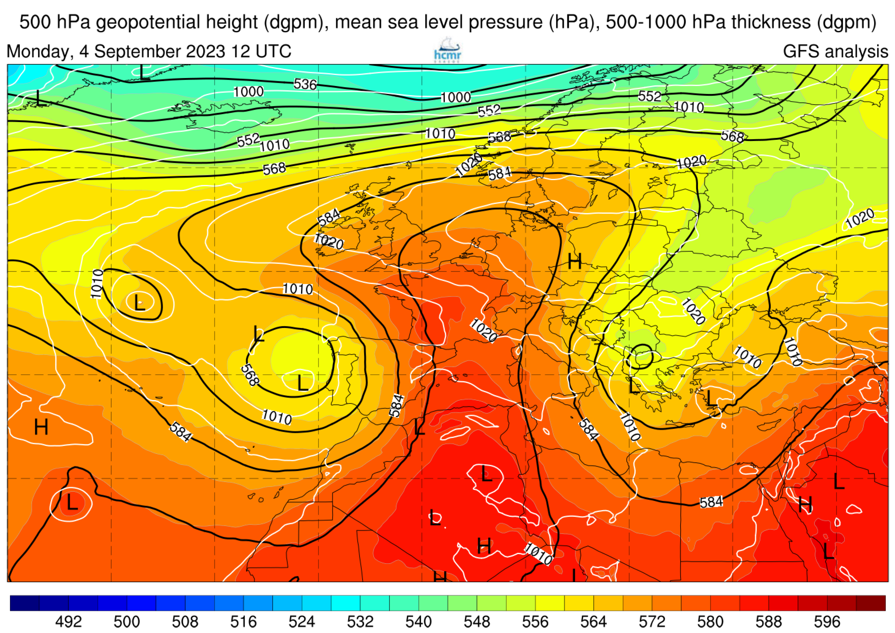
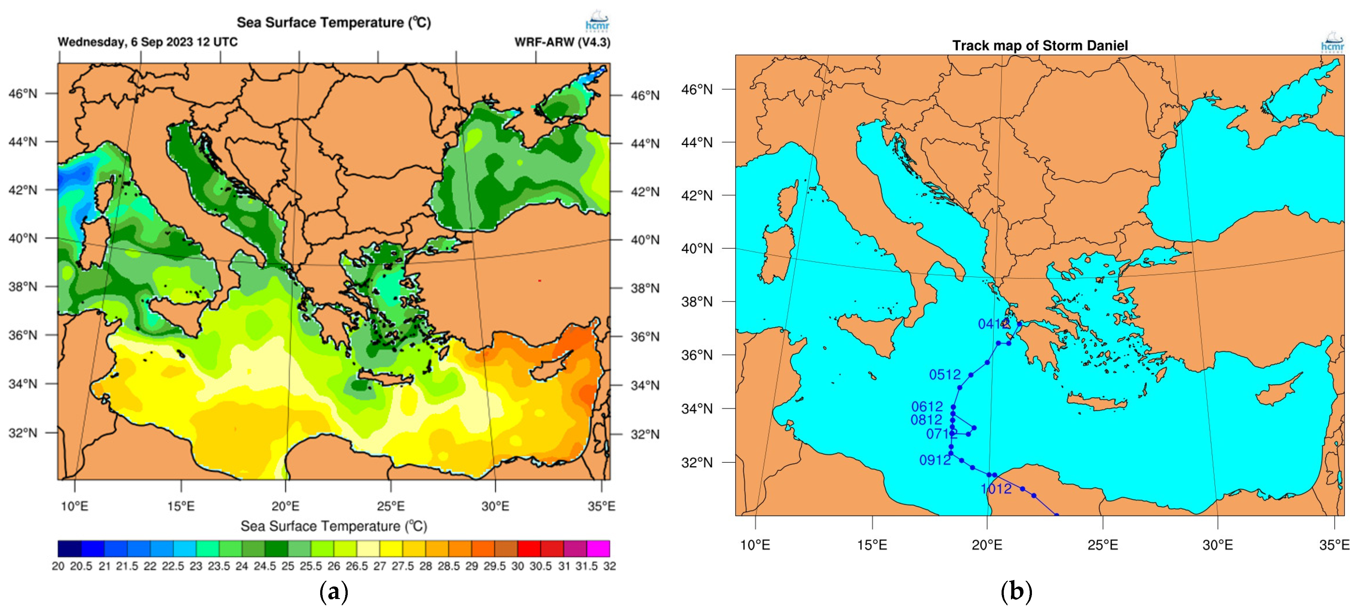
3.1.1. Overview and Physical Interpretation

From 3 to 8 September 2023, a depression (named Daniel) affected the Southeastern Mediterranean region. The general synoptic conditions in Europe at that time indicated the formation of a deep upper-level barometric low along the west coast of the Iberian Peninsula that affected the jet stream and caused it to bend and weaken. Ahead of this low to the east, an upper-level ridge begins to strengthen relatively rapidly, transporting warm and moist air from North Africa to Europe. This situation favored the establishment of a blocking anticyclone that spread over Western, Central, and Northern Europe. Figure 3 shows that, on 4 September 2023 at 12 UTC, this upper-level weather pattern was fully developed. Because the geopotential height contours at the upper atmosphere associated with this pattern appear to form a shape like the Greek letter Ω, this blocking pattern is known as an omega block. The omega blocking patterns are associated with a long-lasting period of stable weather: hot and clear sky in the middle under the ridge of the omega block and rain and clouds in the areas around the troughs on either side of the omega block.

The particular omega block that developed when the atmosphere and ocean were still warm caused a long period of extreme temperatures for September in areas of Western Europe that lay below the central part of the pattern, and huge amounts of precipitation in the Iberian and Balkan Peninsulas were associated with the two large and deep upper lows on either side of the omega block.

In its early state, Storm Daniel formed over Greece as a deep upper-level low and gradually moved southwest into the Ionian Sea and the Southern Mediterranean. The observed sea surface temperatures (SST) across the Southern and Eastern Mediterranean Sea in September remained significantly high, from +2 to +3 °C higher than climatological means.

These exceedingly warm SST across the Ionian and Mediterranean Seas provided additional heat and moisture that fueled Daniel, allowing it to strengthen further. The large-scale steering flow of Daniel triggered a strong easterly flow of very moist and warm air mass from the warm waters of the Aegean Sea and the Black Sea towards Central Greece, several kilometres away, causing low-level convergence and orographic lifting on the windward areas of mountains. These atmospheric processes produced persistent and heavy rainfall, with the recorded daily and accumulated precipitation between 4 and 7 September 2023 at several meteorological stations, as seen in Table 2. In the next days, Storm Daniel gradually moved over the Ionian Sea and the Southern Mediterranean, where SSTs in the 25–28 °C range were present (Figure 4a). There, under the strong influence of the cut-off trough and the presence of high SST, Storm Daniel developed tropical characteristics, such as an eye and spiral clouds, especially on 9 September. Daniel made landfall near the city of Benghazi in Libya on 10 September. Figure 4b shows the track of the storm as estimated based on the 6-hourly ERA5 analysis of mean sea-level pressure (MSLP).

In Thessaly, Greece, the exceptional storm phenomenon caused extensive regions to be inundated, resulting in 17 casualties, massive damages to livestock, properties, and infrastructures, and a total economic loss on the order of billions of euros. Whole villages were submerged for many days up to weeks after the flood event. Long-term effects on soil fertility and future production may also take place, due to the destruction of crops, fertilizers and mechanical equipment. Given the dominant role of the Thessalian Plain as Greece’s main agricultural area, its breadbasket in particular, it becomes clear that Storm Daniel is expected to have a disastrous impact on the local and national economies [59].

3.1.2. Rainfall Data

By applying the Thiessen polygons’ technique, we estimated the areal precipitation over the Peneus basin, to be 363.9 mm for the four-day event (Table 2). This value, which corresponds to a total water volume of 4026 hm³, was compared with the corresponding value obtained using the ERA5 land precipitation data at a horizontal resolution of 9 km. Particularly, a spatial precipitation depth of 321.4 mm (~10% lower than that estimated by the Thiessen method) was calculated based on the ERA5 land reanalysis data, which corresponds to a total rainfall volume of about 3556 hm³ at the river basin level. It is worth mentioning that, during this 4-day storm event, the basin received about 47% of its mean annual precipitation (780 mm).

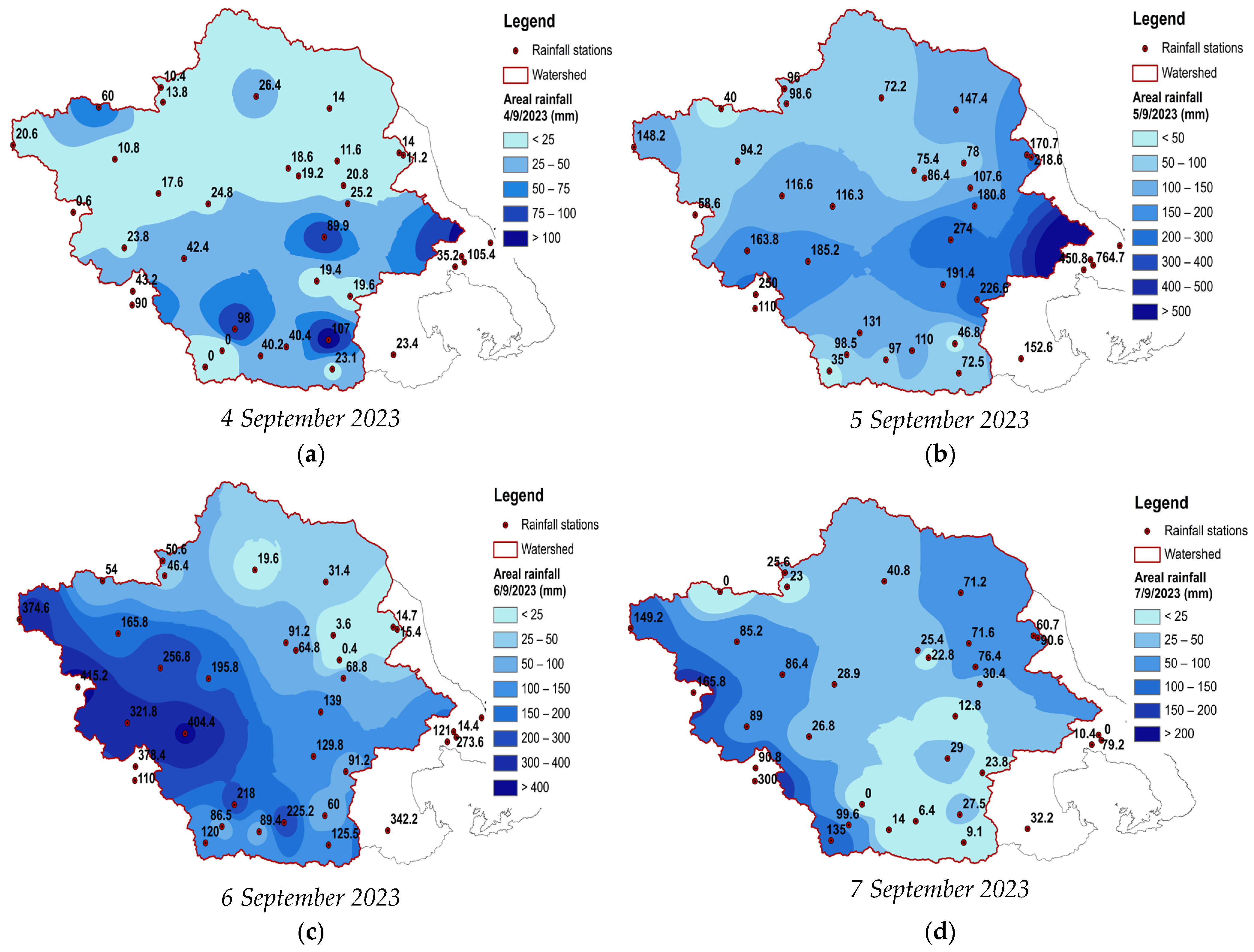
3.1.3. Spatiotemporal Analysis

The spatiotemporal evolution of the storm phenomenon from 4 to 7 September 2023 is depicted by means of the four maps of Figure 5 that have been produced through the inverse weighting distance interpolation method, using the observed point rainfall data of Table 2. On Monday, 4 September, the storm hit the SE part of the basin and then moved west, where the highest accumulated rainfall values were eventually produced. The phenomenon was clearly less intense in the southern and northern parts of the basin. The spatial distribution of the accumulated rainfall is mapped in Figure 6d (lower right map).

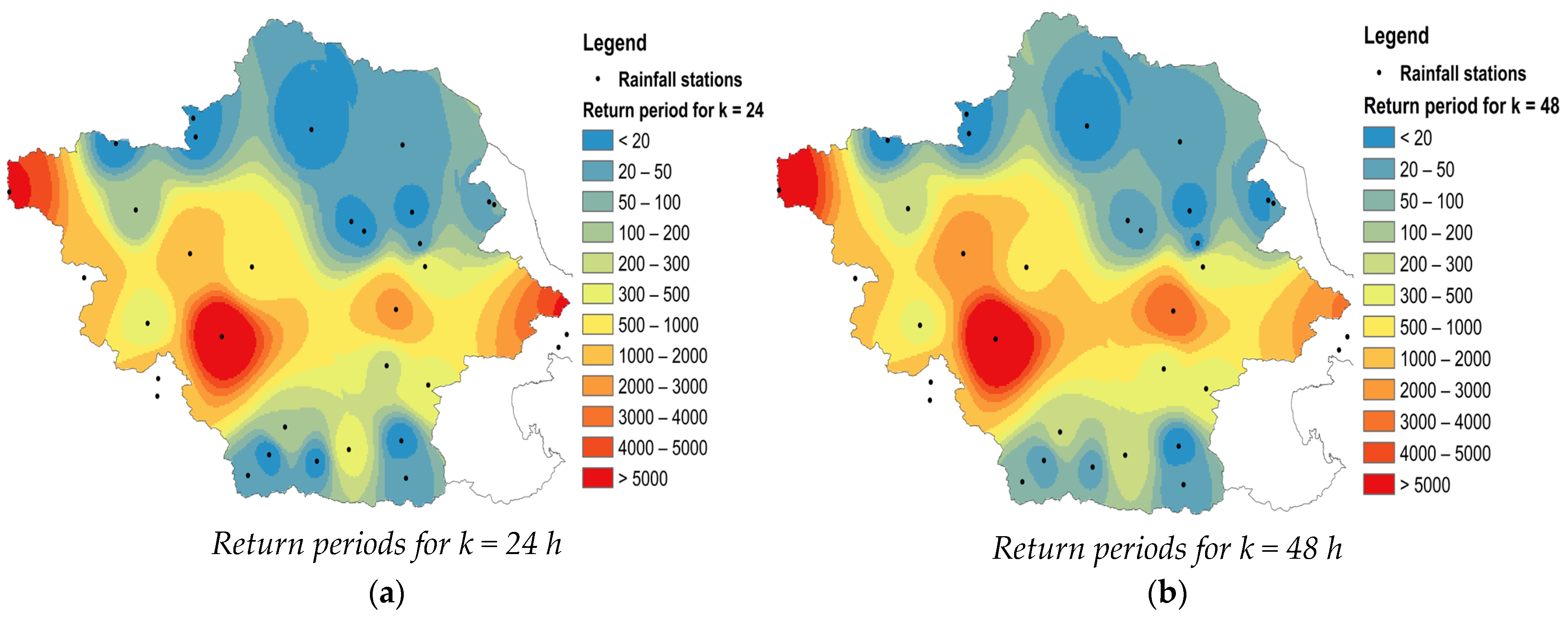
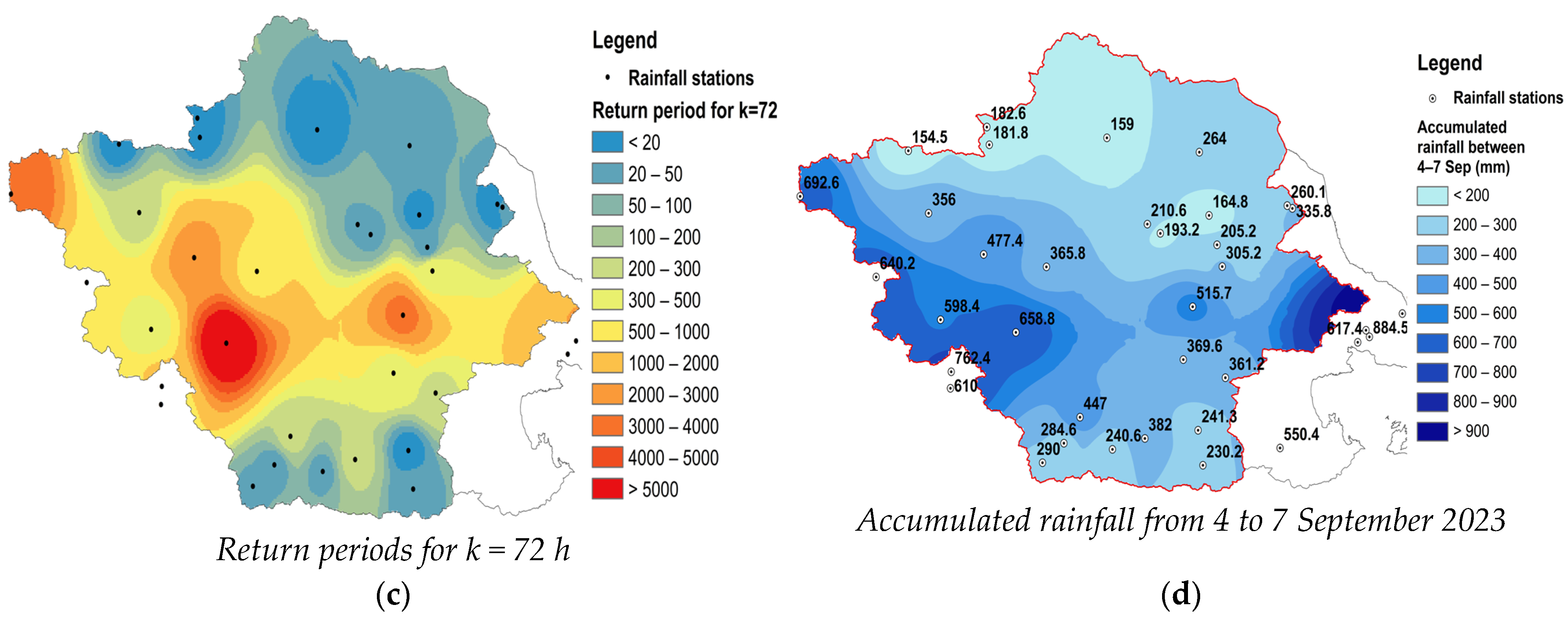
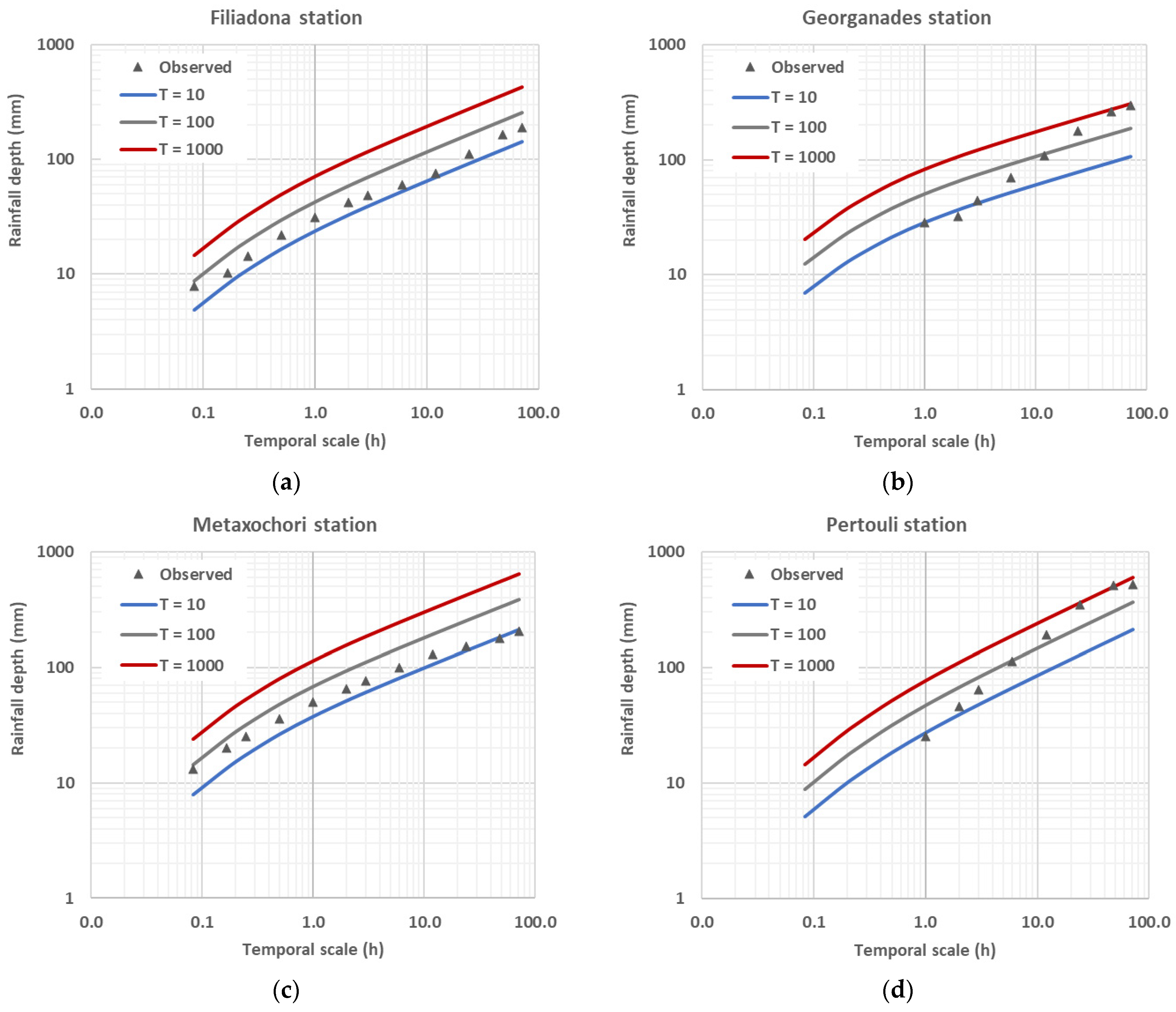
3.1.4. Estimation of Rainfall Return Periods across Stations

The daily values of Table 2, as well as the more detailed data at four stations (Filiadona, Georganades, Metaxochori, and Pertouli), were used to initially estimate the return period of the event at the stations’ locations across the three temporal scales of interest (24, 48, and 72 h), based on the gridded values of ombrian curve parameters across Greece (freely available at https://www.itia.ntua.gr/2273/). To retain consistency to the methodology of the ombrian curves, in which fixed-block instead of moving maxima are applied for the estimations, and following the respective guidelines (Chapter 12 in [53]), an average maximum rainfall depth is estimated for the temporal scale of interest, as derived from the $k/D$ different possible aggregations of the storm event at scale $k$ for a given temporal data resolution $D.$ The associated return periods are obtained by solving Equation (1) for the unknown T. The outcomes of this probabilistic analysis are summarized in

Table 3. Probabilistic analysis across meteorological stations to extract return periods of point and areal rainfall across three temporal scales. Parameters α = 0.18 h and ξ = 0.18 are common for all stations.

Station	Spatially Varying Ombrian Curve Parameter			$\mathbf{Average}\mathbf{Max}.\mathbf{Rainfall}\left(\mathbf{mm}\right)\mathbf{for}\mathbf{Scale}\mathit{k}$			$\mathit{T}$$\left(\mathbf{Years}\right)\mathbf{for}\mathbf{Scale}\mathit{k}$
	$\mathit{\eta }$	$\mathit{\lambda }$ (mm/h)	$\mathit{\beta }$ (years)	24 h	48 h	72 h	24 h	48 h	72 h
Agia	0.619	69.22	0.037	218.6	231.9	266.5	55	24	23
Agiofyllo	0.643	34.94	0.014	60.0	97.3	116.3	3	8	9
Anavra	0.618	42.75	0.017	218.0	289.0	341.7	200	214	225
Anilio	0.560	25.92	0.011	374.6	523.3	597.7	5043	5790	3944
Chalki	0.716	57.57	0.032	180.8	227.8	253.6	361	417	401
Dasochori	0.619	37.58	0.019	98.6	128.7	146.6	13	13	12
Dendra Tyrnavou	0.730	63.36	0.033	86.4	128.4	150.0	16	35	42
Deskati	0.596	33.86	0.017	96.0	126.5	145.2	11	11	10
Domokos	0.615	40.66	0.021	225.2	283.4	316.3	340	284	230
Elassona	0.658	60.12	0.060	72.2	95.2	116.5	6	6	8
Filiadona	0.603	37.46	0.023	125.5	166.3	187.6	32	33	28
Georganades	0.721	54.33	0.021	195.8	268.4	300.9	503	880	880
Gonnoi	0.706	84.74	0.032	147.4	170.1	201.4	25	20	24
Kalampaka	0.641	39.82	0.014	165.8	255.5	289.0	113	256	230
Karditsa City	0.691	58.03	0.023	404.4	510.4	559.9	6354	6878	5816
Karitsa	0.489	24.94	0.015	300.0	355.0	413.3	497	209	162
Loutropigi	0.600	38.21	0.017	99.6	185.6	218.6	9	33	33
Makrinitsa	0.510	50.90	0.041	757.4	956.8	1049.7	6290	3724	2232
Metaxochori	0.619	69.22	0.037	170.7	185.0	210.0	21	11	10
Mouzaki	0.639	63.53	0.017	321.8	448.2	498.3	307	442	365
Neraida	0.620	41.36	0.027	226.6	282.0	308.4	463	374	278
Nessonas	0.734	69.18	0.034	78.0	85.6	112.0	9	6	11
Pertouli	0.539	32.18	0.013	415.2	527.4	565.0	1904	1276	720
Pezoula	0.489	24.19	0.015	378.4	548.8	620.0	1794	1939	1279
Platanioula	0.721	65.21	0.037	91.2	141.6	164.6	16	42	48
Platykampos	0.735	74.03	0.034	107.6	118.2	147.2	23	16	24
Rentina	0.586	34.69	0.017	135.0	205.0	233.3	31	52	44
Skopia	0.619	51.27	0.030	107.0	130.4	167.3	9	7	10
Smokovo	0.619	35.62	0.018	97.0	161.8	188.1	15	41	40
Trikala	0.696	48.45	0.016	256.8	358.3	398.0	1365	2448	2231
Vamvakou	0.661	47.16	0.025	191.4	266.0	300.5	270	410	380
Volos	0.729	106.64	0.029	450.8	528.9	558.4	1737	1497	1143
Zappeio	0.661	43.61	0.026	274.0	388.5	430.9	2167	3731	3151
Areal	0.648	49.99	0.024	143.6	283.0	280.0	44	133	144

, while the return periods across the watershed at the three temporal scales are also depicted in Figure 6a–c.

The point return period values exhibit substantial variability across the examined stations, consistent with the marked spatial variability of extreme rainfall, since they range within up to almost four orders of magnitude, i.e., from 10 up to 7000 years. By looking at their spatial distribution (Figure 6), two clear patterns appear with respect to the rarity of the storm event. In particular, the middle and western parts of the Peneus basin received the most extreme part of the storm, while the rainfall over its northern and southern parts was large, yet not exceptionally extreme. To mitigate the large uncertainty involved in the estimation of the return period on a point basis, we performed the estimation on the regional scale of the Peneus basin, calculating the basin-representative (weighted sum) parameters from the respective parameter grid (Table 3). To estimate the rainfall event at the basin’s scale, we applied the Thiessen polygon method to the individual days of the event (Table 2) and then estimated the average maximum rainfall depth at the different scales, as before. As shown in Table 3, the resulting return periods for the areal rainfall and the temporal scales of 24, 48, and 72 h were 44, 133, and 144 years, respectively. Therefore, the order of magnitude of the overall event is estimated to be up to 150 years, with the rainfall received over the 48 h and 72 h scales being the most severe.

3.1.5. Insight into the Temporal Variability of Return Periods

In order to assess the extremeness of the storm in the time domain, we contrast the average rainfall maxima across multiple scales, following the abovementioned methodology, with the theoretical maxima that are estimated by the ombrian curves, for three characteristic return periods, i.e., T = 10, 100, and 1000 years (Figure 7). This analysis is performed at the four meteorological stations of the study area, where finely resolved data were available. For the Pertouli station, where values towards the end of the event are missing, the maximum values recorded at 24 h, 48 h, and 72 h are used instead of the respective averages. At the two stations lying in the western part of the basin (Georganades and Pertouli), the return periods of rainfall maxima range across three orders of magnitude, namely from about 10 years, and for the hourly scale, to up to 1000 years for the large scales (48 and 72 h). On the other hand, the spread of return periods is smaller (i.e., from 10 up to 100 years), for the two stations in the eastern (Metaxochori) and southern (Filiadona) parts of the basin.

Summarizing the analysis of the rainfall event in terms of return periods, we highlight that the distribution of its extremeness exhibited a noteworthy variability, both in space and time. This reality is in full antithesis with oversimplistic engineering practices that make use of spatially uniform design hyetographs, following the same return period across all temporal scales [60].

3.2. Disentangling the Flood Phenomenon

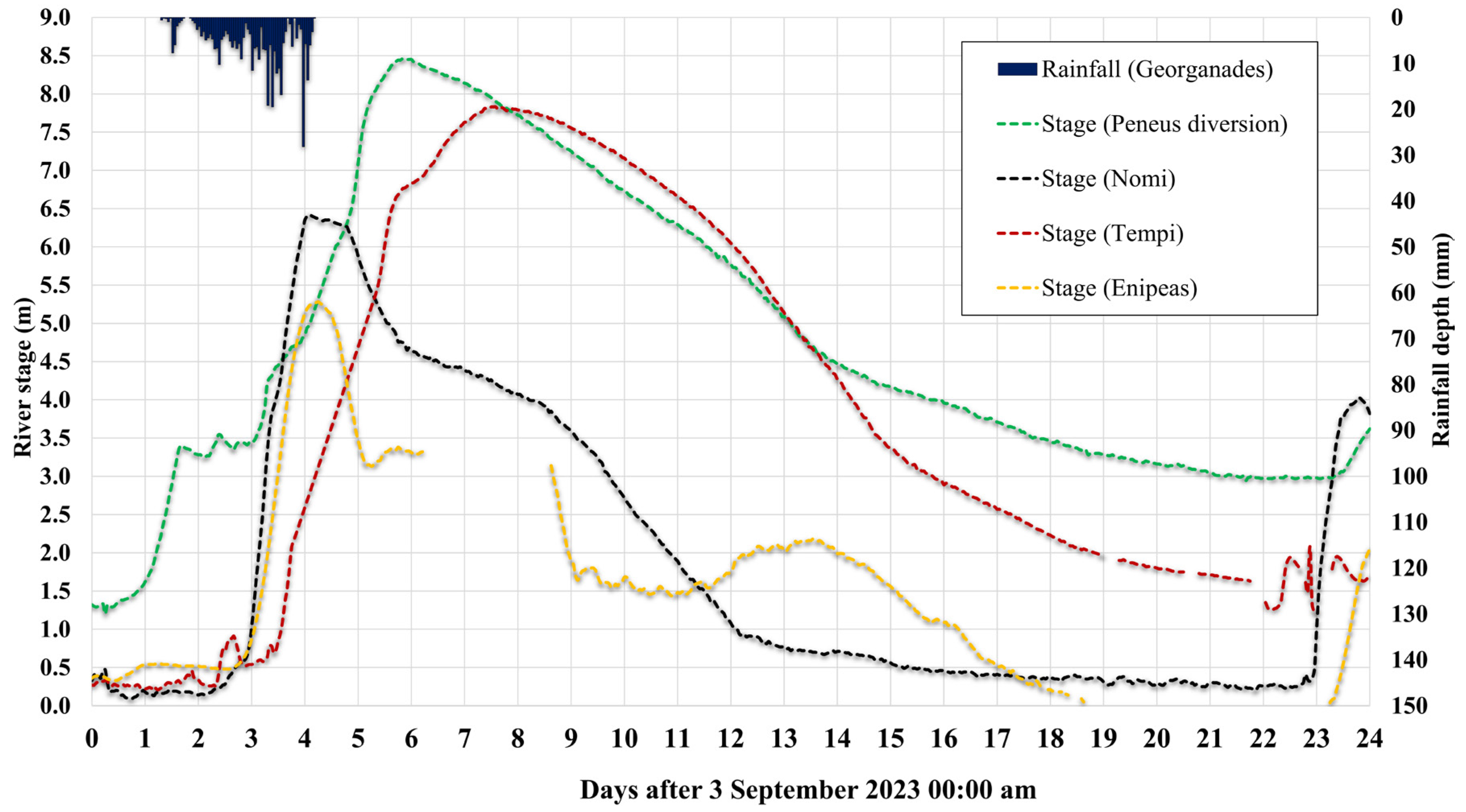
3.2.1. Stage Data

We depicted the stage hydrographs at all monitoring stations in order to obtain a first picture of the propagation of the flood event across the basin, and also extracted their main characteristics, as shown in

Table 4. Characteristic flood quantities at monitoring sites.

Monitoring Station	Max. Stage (m)	Date/Time at Peak	Time to Peak (h)	Max. Discharge (m3/s)
Tempi	7.83	10 September 14:30	126	1947.1
Peneus diversion	8.47	8 September 20:30	130	-
Nomi	6.42	7 September 2:00	38	998.6
Magoula	5.03	6 September 8:00	23	206.9
Enipeas	5.33	7 September 5:00	39	1190.0
Theopetra	2.49	7 September 4:00	12	140.9

. By accounting for the time at peak and then empirically detecting the time when the direct runoff started, we estimated the duration of the rising limb for each generated hydrograph, by subtracting the respective points in time. It should be noted that for the case of Theopetra, where a double-peak hydrograph was generated. The first peak was selected to estimate the rising time, as this was considered to be unbiased from the antecedent flow conditions.

Figure 8 presents the evolution of stage observations along the stations installed across the main course of the Peneus River (from upstream to downstream: Nomi, Peneus diversion, Tempi) as well as at the outlet of Enipeas River, which is the most important tributary of Peneus. We also illustrate the observed hyetograph at Georganades, which lies in the central part of the basin. This station recorded a total rainfall depth of 365.8 mm throughout the event, which is very close to the mean spatial value of 364.2 mm (Table 1). The rainfall peak took place on 6 September 2023, at 23:00 p.m. EET.

Key conclusions drawn from visual inspection of stage data across the four stations are:

The stage hydrograph at Nomi station, which is the most upstream monitoring site on the main course of the Peneus River, indicated, from visual inspection, a time to peak of approximately 37.5 h and a time base of about 14 days. The peak occurred on 7 September at 02:00 a.m. EET, when the river level rose approximately 6.4 m above the bed, which is very close to the absolute safety limit for overflowing.

The Peneus diversion monitoring station, located in the northeastern part of Larissa city, exhibited a maximum depth of 8.47 m on 8 September at 20:30 p.m. EET, thus corresponding to a time to peak of about 130 h. The difference of time peaks with respect to the upstream station (Nomi) was about 42 h. This difference is reasonable since the upstream drainage area is much larger, while the slopes become milder towards the river mouth. We note that a new flood event occurred by the end of September, thus making it difficult to estimate the time base of the hydrograph, since the two events are overlapping. Limited overflow was observed during the event in the area around the station.

Regarding the most downstream station, Tempi, its maximum recorded stage was 8.47 m, on 10 September at 14:00 p.m. EET. This corresponds to a 39 h lag time in relation to the observed peak in the upstream gauging station (Peneus diversion), at a distance of approximately 53 km. The rising time of the hydrograph is about five days, while the total duration of the flood exceeds 25 days.

Finally, the observed stages at Enipeas station followed a similar pattern to Nomi and exhibited a maximum depth of 5.33 m (the stage records are not continuous due to power outages). We note that, through the passage of Storm Daniel, extended parts along the lower course of Enipeas overflowed, causing significant damage to settlements and agricultural areas.

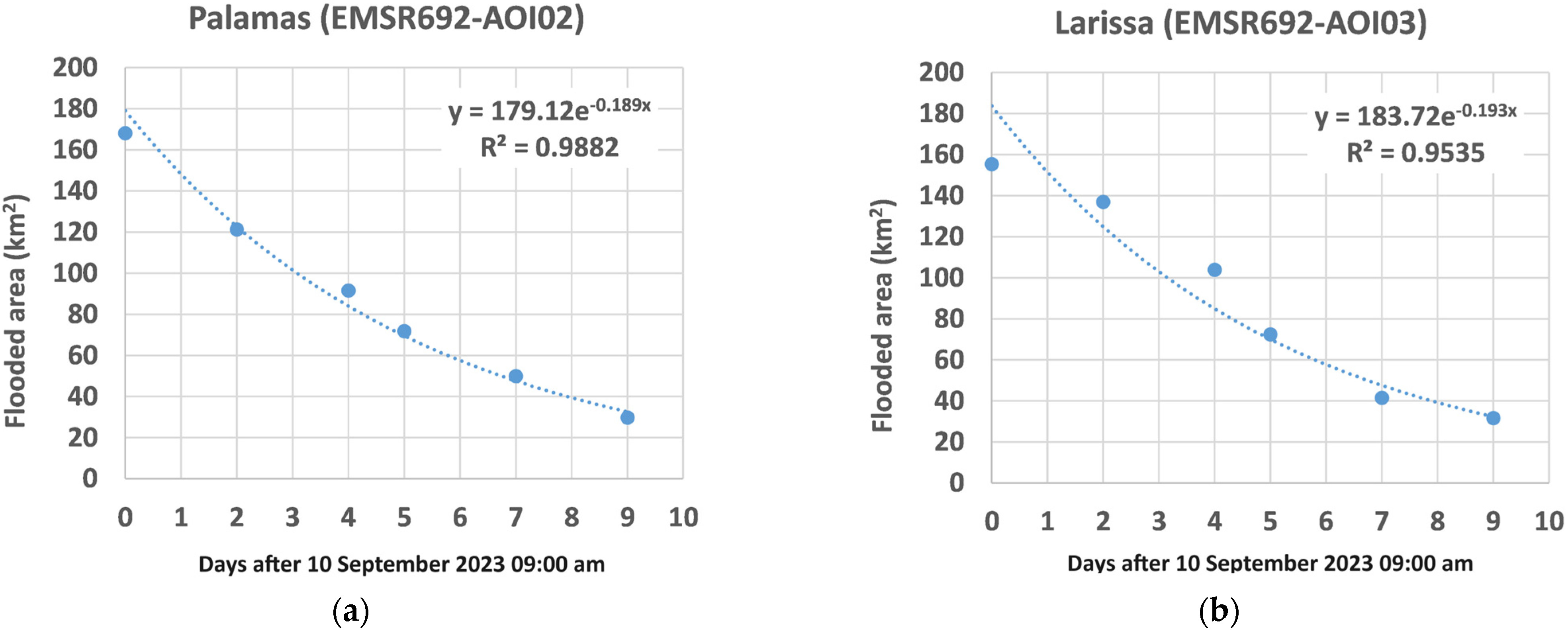
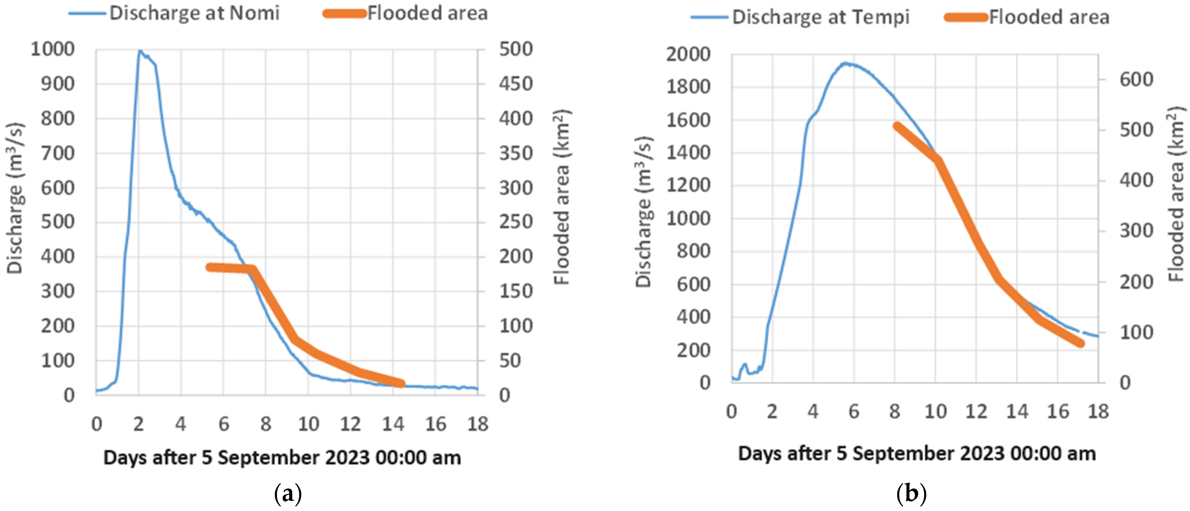
3.2.2. Discharge Analysis and Flood-Inundation Data

By applying the established rating curves at all monitoring sites, we computed the discharge time series based on stage observations and then extracted the estimated peak flows (Table 4). Considering four representative monitoring stations over the hydrographic network (from upstream to downstream: Magoula, Nomi, Enipeas, and Tempi), the peak flows are 207, 998, 1190, and 1947 m³/s, respectively.

An approximate estimation of the flood volumes produced by Storm Daniel is only feasible for the two stations along the main course of Peneus, i.e., Nomi and Tempi, since a significant part of data at Enipeas is missing (Figure 8). By considering the discharge data until the following flood event, starting on 26 September 2023 at 9:00 a.m. EET, the water volumes sum up to 412 and 1538 hm³, at Nomi and Tempi, respectively, corresponding to runoff depths 96.7 and 76.0 mm, respectively. Considering the unprecedented heaviness of the storm event, these values are probably lower than expected due to substantial attenuations from the terrain’s relief (mild up to negligible slopes) as well as due to retentions and overflows across the drainage system.

As already mentioned, Storm Daniel caused extensive damage over the study area, since large parts of the basin were inundated. In the overall region of Thessaly, the total extent of flooded areas exceeded 1150 km² [59]. To assess in more detail the spatiotemporal evolution of the inundation process, we retrieved associated data from the Emergency Management Service of Copernicus (https://rapidmapping.emergency.copernicus.eu/EMSR692, accessed on 22 March 2024) regarding three major domains of interest (from upstream to downstream: Karditsa, Palamas, and Larissa). All drain into the Peneus a little upstream of the three monitoring stations. The data are summarized in

Table 5. Flooded areas (ha) over Thessaly after Storm Daniel, retrieved by the Emergency Management Service of Copernicus (https://rapidmapping.emergency.copernicus.eu/EMSR692, accessed on 22 March 2024). Values in italics are estimated via interpolation.

Date	Karditsa (EMSR692-AOI0)	Palamas (EMSR692-AOI02)	Larissa (EMSR692-AOI03)	Total
10 September 2023 9:00	18,519	16,808	15,532	50,859
12 September 2023 9:00	18,251	12,129	13,691	44,072
14 September 2023 9:00	8018	9157	10,383	27,558
15 September 2023 9:00	6000	7183	7244	20,427
17 September 2023 9:00	3315	4988	4156	12,459
19 September 2023 9:00	1700	2982	3163	7845

.

As shown in Figure 9, the inundated areas exhibit a common behaviour with respect to their drainage dynamics, which are well-approximated by negatively exponential laws. Also, by putting the flooded-area data side by side with flow hydrographs, similar patterns are derived, indicating that the flood recession is significantly dictated by the associated drainage mechanisms (Figure 10).

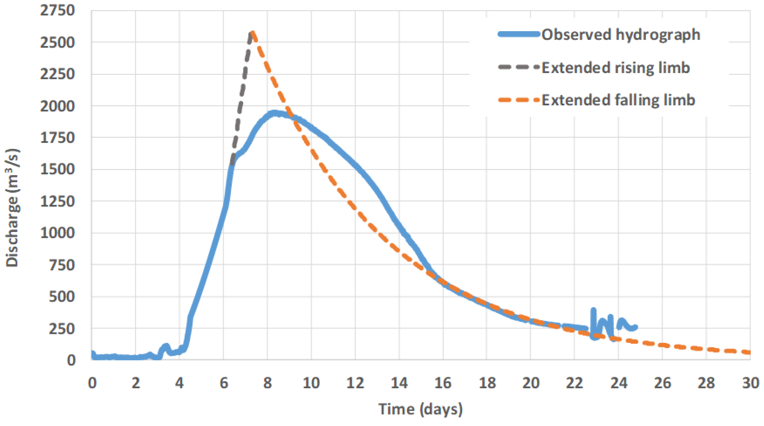
3.2.3. Insight into the Outflow Hydrograph (Tempi Station)

Tempi station is located very close to the river mouth and, therefore, can provide a good image of the overall response of the river basin. In this respect, we analyse the shape of the flow hydrograph, in an attempt to associate its individual components with specific hydrological mechanisms.

A hydrograph can generally be decomposed into rising and recession limbs, representing the direct response of the basin against rainfall events and the delayed flows due to regulation processes, respectively [61]. An important feature is the time at which the direct runoff ceases, which allows separating the baseflow from the total hydrograph, with the aim of estimating the flood runoff component induced by the storm event. The literature offers several approaches for the estimation of the falling limb duration, either based on empirically derived formulas or through visual inspection, by determining the time at which the falling limb of the hydrograph becomes “milder” [62]. A well-known analytical approach uses the scaling law proposed by Linsley et al. [63] (see also [64]), which reads $N={0.8A}^{0.2}$, where N is the number of days from the peak of the hydrograph and up to the point where the surface runoff finishes and A is the area of the upstream catchment in km². Since the drainage area upstream of Tempi is 10,591 km², the above formula yields N = 5.1 days. This value strongly underestimates reality, given that even 20 days after the event, the actual recession limb at this station was far from attenuated, (Figure 8).

Regarding the total hydrograph partitioning into flood runoff and baseflow, this task is subject to multiple ambiguities, mostly related to the selection of the final point of the direct runoff. For single-peak hydrographs and isolated events, the straight-line graphical method constitutes a popular and well-documented approach; in contrast, difficulties arise in the interpretation of surface and baseflow interactions in the case of complex, multi-peak hydrographs [65,66].

As shown in Figure 8, the falling limbs of all observed hydrographs are not smooth, yet they exhibit multi-recession behaviours (i.e., changing slopes), following the drainage patterns of inundated areas (Figure 10). Regarding the hydrograph at the outlet, Tempi (Figure 11), at least three different recession behaviours are detected.

In the range from 1400 to 700 m³/s, the optimized value of recession parameter k was 0.248 d⁻¹, while for lower discharge values, k was found to be 0.165 d⁻¹. The difference is quite significant and should be attributed to different delay mechanisms, probably the slow drainage of inundated areas over the terrain and the overall drainage of the basin by means of groundwater flow, which is the slowest runoff mechanism.

Next, following the idea by Sakki et al. [67], we attempted to reconstruct the hypothetical response of the Peneus basin in the absence of retentions due to inundations, as well as in the absence of the flood event that took place 23 days after Storm Daniel. In this respect, we extrapolated the groundwater recession function in the forward and backward directions and also extrapolated the rising limb forward, assuming that this is approximated by a linear function (Figure 11).

Through visual inspection, we conclude that the base time reaches or even exceeds 30 days, while the use of the theoretical decay function after day 22 as a proxy of the real hydrograph results in a total runoff volume of about 1670 hm³. By contrasting the observed peak flow (1950 m³/s) with the theoretical one (~2600 m³/s), we conclude that these may have contributed to a peak flow reduction of up to 25%. By subtracting the observed discharge values from the theoretical ones, derived through the extrapolated falling limb (Figure 10), we can also estimate the excess flood volume, which is about 120 hm³. By dividing by the totally flooded area (about 500 km², Table 5), we get an average inundation depth of about 25 cm, which is reasonable. Eventually, this quantity has been temporarily retained in the inundated areas and returned to the river network with a time delay of several days, thus resulting in a significantly smoother response of the overall hydrological system. In practical terms, this highlights the key importance of promoting the configuration of artificial retention basins as non-structural measures towards flood risk mitigation over the study area [68].

Another interesting outcome derives from expressing the reconstructed flood hydrograph in dimensionless terms, i.e., by dividing the time values by the theoretical time to peak and the discharge values by the theoretical peak discharge. This was contrasted with several synthetic unit hydrographs that are commonly applied in Greece in flood design and risk-assessment studies, also including the implementation of the 2007/60/EC Flood Directive. As shown in Figure 12, the best-fitted one is the so-called Delmarva Unit Hydrograph (DUH), obtained from the suite of dimensionless unit hydrographs developed by the U.S. Natural Resources Conservation Service [69]. While NRCS generally proposes the use of a standard shape, namely the dimensionless curvilinear unit hydrograph, also referred to as PRF484, for areas where the local topography is flat and where considerable surface storage is available, it strongly suggests the use of DUH, which is much smoother (the associated peak rate factor is 284 instead of 484) [70]. Our analysis indicates that this hydrograph is very suitable for areas such as Thessaly and similar ones in Greece for properly representing the highly complex flood-retention processes across large-scale agricultural basins.

3.2.4. Rainfall–Runoff Analysis and Comparison with Past Events

The next stage of investigations consists of exploiting the results derived from the above-described hydrograph reconstruction method to perform an overall water balance assessment, with respect to the proportion of the total storm volume finally transformed into surface runoff and that corresponds to the hydrological losses. The estimated flood runoff volume that passed through Tempi station over the 30-day period is 1670 hm³, which corresponds to a runoff depth of 157.4 mm. On the other hand, the total rainfall depth over the entire river basin was estimated to be 363.9 mm (Table 1). In this vein, approximately 43% of the total rainfall volume was transformed into runoff. This ratio is reasonable for such an extraordinary rainfall quantity.

By solving the SCS runoff curve number Equations (3) and (4), we get $CN=47$, which is adjusted to a reference value of 68 when accounting for dry antecedent soil moisture conditions at the beginning of the storm event. We note that, by considering the average soil moisture conditions, according to the NRCS standards and thus applying the reference CN value (i.e., 68) to the same rainfall depth, we would get a flood depth of up to 250 mm. Nevertheless, the reference CN value is yet quite smaller than recent estimations provided within the implementation of the 2007/60/EC Flood Directive in Greece, considering an average CN up to 80 for Thessaly. This difference should be attributed to the blind use of flood recipes that have been developed and validated under different geomorphological conditions and hydroclimatic regimes [71]. In particular, the ignoring of the dominant role of slope and other retention mechanisms within the estimation of CN may lead to estimations that are far away from reality [72].

Considering the time delay between the peak flow records at the gauging stations Nomi (upstream) and Tempi (downstream) and measuring the corresponding distance, an estimation of the apparent flood-wave celerity was made. This empirically derived apparent flood-wave celerity in this reach of the river was approximately 0.44 m/s (distance between stations: 135 km) and expresses the peak lag of the flood between the two stations and not the actual wave celerity during the event. A series of factors, such as overflows along the course of the river, significant inflows from sub-basins between the examined locations, and the varying rainfall’s spatiotemporal patterns throughout the basin affected the above estimate. In particular, two important sub-basins (Enipeas and Titarisios) contributed significant volumes of water in the main river reach between Nomi and Tempi stations, with different peak flows in terms of magnitude and timing in relation to the main flood wave, while large volumes of water overflowed (at least) at three different spots along the main branch (on 6 September 2023 close to the Enipeas confluence, on 7 September 2023 close to the city of Larissa and on 8 September 2023 close to the Lake Karla diversion canal). Further, based on the maximum discharge values and the corresponding cross-sectional areas at the gauging stations in Nomi and Tempi, local flow-velocity values were slightly above 2 and 3 m/s, respectively, which are considerably higher than the estimated flood-wave celerity based on the apparent peak flow travel speed.

Actually, flood-wave hydraulic theory shows that wave celerity generally exceeds the mean cross-sectional velocity [73]. Therefore, to analyse accurately the evolution of the flood-wave propagation and estimate credible celerity values, a hydraulic simulation should be performed for the main Peneus river reach (with actual field geometry) also considering lateral inflows from the main sub-basins and various overflows along the river.

In this study, an attempt was also made to compare the current flood against past events of high magnitude in the area, to gain insights into the comparative response of the Peneus river basin. For this purpose, four events in total, which occurred over the last few years, were selected for further analysis, among which the catastrophic flood event induced by Ianos Medicane that resulted in four casualties and extended damage in the western and central parts of Greece. The selection of the events was based upon the simultaneous availability of water depth and discharge data at both the Nomi and Tempi stations, whereas a prerequisite of a maximum water depth of at least 4 m at Nomi was also considered to ensure high magnitude occurrence and, thus, the comparability of the events.

The selected events were compared against each other with respect to the maximum recorded water depth and discharge values at the Nomi and Tempi stations, as well as regarding the estimated peak flow travel times.

The results show that the travel time of the peak flow between Nomi and Tempi stations exhibits marked discrepancies between the examined events, ranging from 40 up to 84.5 h (

Table 6. Comparison of Storm Daniel against past events with respect to maximum depths and flows along the Nomi–Tempi river segment and estimated direct runoff volume at the outlet station (Tempi).

Examined Event	Monitoring Station	Max Flow (m3/s)	Max Depth (m)	Time at Max	Peak Flow Travel Time (h)	Direct Runoff Volume (hm3)
September 2023 (Daniel)	Nomi	999	6.42	7 September 2023 2:00	84.5
	Tempi	1947	7.83	10 September 2023 14:30		1670
September 2020 (Ianos)	Nomi	523	4.39	19 September 2020 20:30	64.5
	Tempi	787	3.92	22 September 2020 13:00		317
April 2020	Nomi	525	4.40	5 April 2020 23:30	58.5
	Tempi	913	4.39	8 April 2020 10:00
January 2021, 1st peak	Nomi	543	4.49	4 January 2021 21:30	53.5
	Tempi	584	3.12	7 January 2021 3:00
January 2021, 2nd peak	Nomi	648	4.99	12 January 2021 15:00	45.0
	Tempi	704	3.60	14 January 2021 12:00
November–December 2021	Nomi	557	4.56	30 November 2021 16:30	40.0
	Tempi	430	2.47	2 December 2021 8:30

). Storm Daniel presented the longest travel time, which is most probably due to the extended flooding that occurred in a large part of the catchment. The second lower travel time was observed in the case of Ianos Medicane, while for the rest of the events, the travel times were lower (between 40 and 58.5 h).

Although these results are only indicative, because of the limited events analysed, the availability of this kind of data shows enormous potential for the establishment of a flood alert and forecasting tool.

Regarding the total discharge volume reaching the outlet of the Peneus River catchment, an estimation was also made for the Ianos event, giving approximately 317 hm³. This is approximately 19% of the estimated flood runoff volume in the case of Storm Daniel, thus giving a rough idea of the extreme nature of the latter event.

4. Discussion

4.1. Early Warning Potential through Automatic Monitoring Networks

The significant impacts caused by extreme flood events such as Daniel, especially in areas that are highly vulnerable due to natural and socioeconomic conditions, necessitate the establishment of reliable flood early-warning systems (FEWS) as a highly important non-structural means for protecting human life, infrastructure, and the local economy.

Several studies identified that the use of FEWS can reduce mortality from natural disasters [74,75], especially in countries with limited or inefficient anti-flood infrastructure. Moreover, Schroter et al. [76] estimated that a 12 h flood warning lead time can provide a 60% reduction in damages while a 1 h lead time can offer a 20% reduction.

Successful examples of FEWS exist in many countries worldwide, including the Flanders region in Belgium, the Red Sea Mountains in Egypt, and the Inner Niger Delta in Mali [77]. The Global Flash Flood Guidance Program is a recent initiative [78], aiming to offer flash flood early-warning systems, mainly in small-scale basins that are prone to flash floods. This infrastructure has been implemented already in a large number of countries worldwide and continues its expansion [79]. China has invested more than 4 billion USD for mitigating flash floods with the establishment of FEWS as a primary activity in 2058 counties [80]. Most of these systems use a combination of water-level sensors, weather forecasting, and hydrologic models, while the maximum warning lead time ranges from 48 h to several weeks. Regarding funding mechanisms for FEWS, central governments are the primary source of financial support (31% of the total), followed by international donors (23%) and local governments (13%), while national research funding accounts for 8% of the associated costs [75].

Nevertheless, a recent study by Perera et al. [75] illustrated that only half of the basins covered by FEWS have streamflow gauges, of which 38% are telemetric, 52% manual, and 10% semi-automatic, while remote-sensing tools are used in 23% of the surveyed FEWS. In this respect, networks of automatic water-monitoring stations are essential infrastructures for near real-time monitoring and timely warning notifications regarding flood-risk phenomena, since they incorporate sensors that record and transmit at regular time intervals (e.g., every 15–30–60 min) the water level and velocity measurements in rivers, streams, dams, or other water bodies. If the monitoring system is integrated with rainfall gauges and weather forecasts, the relevant flood warnings can be available up to 2–3 days before the actual event. Such early-warning systems can also be linked with web applications or mobile devices that can disseminate the information and the alerts to a wider audience, further enhancing the resilience of the people and the institutions to cope with floods.

In Greece, there are various networks of automatic water-monitoring locations with early-warning capabilities that have more than 100 operational stations, controlled by different authorities/bodies [81]. We argue that their integration into a single platform will facilitate the establishment of a country-wide FEWS that will support national and local authorities to mitigate flood-risk impacts effectively. This option may be offered by an extension of the Open Hydrosystem Information Network (https://openhi.net/en/) [52,82], which is a part of the Research Infrastructure “Hellenic Integrated Marine Inland water Observing Forecasting and offshore Technology System” (HIMIOFoTS; https://www.himiofots.gr/).

4.2. Daniel Flood Event

The extended lower parts of the Thessaly Plain, as configured after a series of large-scale reclamation works, constructed since the beginning of the 20th century, is a highly-modified hydrosystem that is still too vulnerable to floods. During the last decades, several severe flood events have occurred, causing significant damages, the most recent of which (Storm Daniel) is investigated in this paper.

Storm Daniel was an extreme event, both in terms of rainfall values and duration (more than 72 h). It resulted from exceptional atmospheric conditions combined with significantly high sea temperatures, causing persistent and heavy rainfall in Central Greece, including Thessaly.

To quantify the probability of this event, we investigated the observed records of 39 meteorological stations in the area of interest and took advantage of the recently updated ombrian curves across the Greek territory, which are based on an innovative probabilistic–stochastic framework. The analyses showed a substantial spatiotemporal variability of the rainfall event over the study area, with point return periods ranging from 10 up to more than 1000 years. At the three-day scale, the areal average rainfall depth received over the entire Peneus river basin corresponds to a return period of up to 150 years.

Furthermore, we retrieved the observed stage hydrographs from six automatic monitoring stations, to examine the associated spatiotemporal evolution of the derived flood event along the Peneus river network. As indicated from our analyses, the time to peak ranged from 10 h in the most upstream stations (Theopetra) to more than 5 days in the most downstream station (Tempi), while the peak flow travel times between stations located in the middle of the basin (Nomi) and the outflow station (Tempi) was 3.5 days. On the other hand, due to the large extent of the basin, its geomorphology (extremely low slopes) and extended retentions across to man-made drainage network, the base time of the flood hydrograph at the outlet exceeded 30 days. The total flood volume that passed through the Tempi station was estimated at 1670 hm³, which corresponds to a runoff depth of about 160 mm, thus approximately 43% of the total rainfall volume was transformed into runoff. We stress that all flood quantities would be probably quite larger if the event occurred under less dry soil-moisture conditions.

Furthermore, on the basis of satellite observations of flood-inundation data, we demonstrated that the shapes of flood hydrographs were significantly dictated by the overflows across the channel network and the associated retention and drainage mechanisms. Finally, by employing empirical extrapolation rules, we also reconstructed the theoretical hydrograph at the basin outlet and contrasted it with specific types of literature-derived unit hydrographs [83,84,85]. Among other practical outcomes, this analysis verified the suitability of the so-called Delmarva Unit Hydrograph by the NRCS for the representation of flood propagation processes across large agricultural basins, instead of commonly used synthetic unit hydrographs.

To highlight the major role of antecedent soil moisture conditions in flood volume production, we applied the NRCS formula for the reference curve number (i.e., $CN=$68), instead of the value derived for dry conditions ($CN=$47). Considering the same value of total rainfall (i.e., 363.9 mm), we would get a significantly larger runoff depth, equal to 250 mm. This quantity is almost 60% larger than the observed one, indicating that the status of the unsaturated zone at the beginning of the rainfall helped to moderate the size of the flood. In contrast, the significantly dry (and warm) past conditions strongly favoured the generation of the exceptional storm event, as already explained in Section 3.1.1. This outcome reveals the importance of combined meteorological and soil conditions, as well as weather types, within the generation of extreme floods, which is an open research topic for further investigation [86].

All these analyses reveal the priceless value of both meteorological and hydrometric information, as the unique means to understand and quantify complex phenomena and provide well-established tools for hydrological design and water-resources management. Hydro-meteorological information was used about 20 years ago for real-time flood forecasting in the relatively small Kephisos river basin (~400 km²), in which the Greater Athens area is located [87]. However, to our knowledge, this is the first attempt in Greece to study really extreme flood phenomena at this spatial scale (~10,000 km²) on the basis of real data and not simply by relying on theoretical and empirical models.

Finally, the specific characteristics of the flood-prone area of Thessaly (low response time, potential for retentions) make clear the necessity for improving the existing monitoring network towards a more operational use. This should involve the development of a notification system for alerting authorities and communities, in order to take timely and appropriate actions, such as evacuating people, securing assets, deploying resources, or implementing emergency plans (e.g., controlled flooding of agricultural areas).

References

1. Jonkman, S.N. Global perspectives on loss of human life caused by floods. Nat. Hazards 2005, 34, 151–175. [Google Scholar] [CrossRef]
2. Petrucci, O. Factors leading to the occurrence of flood fatalities: A systematic review of research papers published between 2010 and 2020. Nat. Hazards Earth Syst. Sci. 2022, 22, 71–83. [Google Scholar] [CrossRef]
3. Ghimire, E.; Sharma, S.; Lamichhane, N. Evaluation of one-dimensional and two-dimensional HEC-RAS models to predict flood travel time and inundation area for flood warning system. ISH J. Hydraul. Eng. 2022, 28, 110–126. [Google Scholar] [CrossRef]
4. Merz, B.; Blöschl, G.; Vorogushyn, S.; Dottori, F.; Aerts, J.C.; Bates, P.; Bertola, M.; Kemter, M.; Kreibich, H.; Lall, U.; et al. Causes, impacts and patterns of disastrous river floods. Nat. Rev. Earth Environ. 2021, 2, 592–609. [Google Scholar] [CrossRef]
5. Papagiannaki, K.; Petrucci, O.; Diakakis, M.; Kotroni, V.; Aceto, L.; Bianchi, C.; Brázdil, R.; Gelabert, M.G.; Inbar, M.; Kahraman, A.; et al. Developing a large-scale dataset of flood fatalities for territories in the Euro-Mediterranean region, FFEM-DB. Sci. Data 2022, 9, 166. [Google Scholar] [CrossRef] [PubMed]
6. Yang, Z.; Huang, W.; McKenzie, J.E.; Xu, R.; Yu, P.; Ye, T.; Wen, B.; Gasparrini, A.; Armstrong, B.; Tong, S.; et al. Mortality risks associated with floods in 761 communities worldwide: Time series study. BMJ 2023, 383, e075081. [Google Scholar] [CrossRef]
7. Diakakis, M.; Deligiannakis, G.; Antoniadis, Z.; Melaki, M.; Katsetsiadou, N.K.; Andreadakis, E.; Spyrou, N.I.; Gogou, M. Proposal of a flash flood impact severity scale for the classification and mapping of flash flood impacts. J. Hydrol. 2020, 590, 125452. [Google Scholar] [CrossRef]
8. Gaume, E.; Bain, V.; Bernardara, P.; Newinger, O.; Barbuc, M.; Bateman, A.; Blaškovičová, L.; Blöschl, G.; Borga, M.; Dumitrescu, A.; et al. A compilation of data on European flash floods. J. Hydrol. 2009, 367, 70–78. [Google Scholar] [CrossRef]
9. Tegos, A.; Ziogas, A.; Bellos, V.; Tzimas, A. Forensic Hydrology: A Complete Reconstruction of an Extreme Flood Event in Data-Scarce Area. Hydrology 2022, 9, 93. [Google Scholar] [CrossRef]
10. Avila-Aceves, E.; Plata-Rocha, W.; Monjardin-Armenta, S.A.; Rangel-Peraza, J.G. Geospatial modelling of floods: A literature review. Stoch. Environ. Res. Risk Assess. 2023, 37, 4109–4128. [Google Scholar] [CrossRef]
11. Mård, J.; Di Baldassarre, G.; Mazzoleni, M. Nighttime light data reveal how flood protection shapes human proximity to rivers. Sci. Adv. 2018, 4, eaar5779. [Google Scholar] [CrossRef] [PubMed]
12. Li, S.; Sun, D.; Goldberg, M.D.; Sjoberg, B.; Santek, D.; Hoffman, J.P.; DeWeese, M.; Restrepo, P.; Lindsey, S.; Holloway, E. Automatic near real-time flood detection using Suomi-NPP/VIIRS data. Remote Sens. Environ. 2018, 204, 672–689. [Google Scholar] [CrossRef]
13. Pabi, O.; Egyir, S.; Attua, E.M. Flood hazard response to scenarios of rainfall dynamics and land use and land cover change in an urbanized river basin in Accra, Ghana. City Environ. Interact. 2021, 12, 100075. [Google Scholar] [CrossRef]
14. Zelentsov, V.; Pimanov, I.; Potryasaev, S.; Sokolov, B.; Cherkas, S.; Alabyan, A.; Belikov, V.; Krylenko, I. River flood forecasting system: An interdisciplinary approach. In Flood Monitoring through Remote Sensing; Springer: Cham, Switzerland, 2018; pp. 81–100. [Google Scholar] [CrossRef]
15. Barredo, J.I. Normalised flood losses in Europe: 1970–2006. Nat. Hazards Earth Syst. Sci. 2009, 9, 97–104. [Google Scholar] [CrossRef]
16. Arriagada, L.; Rojas, O.; Arumí, J.L.; Munizaga, J.; Rojas, C.; Farias, L.; Vega, C. A new method to evaluate the vulnerability of watersheds facing several stressors: A case study in mediterranean Chile. Sci. Total Environ. 2019, 651, 1517–1533. [Google Scholar] [CrossRef] [PubMed]
17. Stefanidis, S.; Alexandridis, V.; Theodoridou, T. Flood Exposure of Residential Areas and Infrastructure in Greece. Hydrology 2022, 9, 145. [Google Scholar] [CrossRef]
18. Abdi-Dehkordi, M.; Bozorg-Haddad, O.; Salavitabar, A.; Mohammad-Azari, S.; Goharian, E. Development of flood mitigation strategies toward sustainable development. Nat. Hazards 2021, 108, 2543–2567. [Google Scholar] [CrossRef]
19. Jacob, X.K.; Bisht, D.S.; Chatterjee, C.; Raghuwanshi, N.S. Hydrodynamic Modeling for Flood Hazard Assessment in a Data Scarce Region: A Case Study of Bharathapuzha River Basin. Environ. Model. Assess. 2020, 25, 97–114. [Google Scholar] [CrossRef]
20. Mourato, S.; Fernandez, P.; Marques, F.; Rocha, A.; Pereira, L. An interactive Web-GIS fluvial flood forecast and alert system in operation in Portugal. Int. J. Disaster Risk Reduct. 2021, 58, 102201. [Google Scholar] [CrossRef]
21. Nam, D.H.; Mai, D.T.; Udo, K.; Mano, A. Short-term flood inundation prediction using hydrologic-hydraulic models forced with downscaled rainfall from global NWP. Hydrol. Process. 2014, 28, 5844–5859. [Google Scholar] [CrossRef]
22. Bruen, M.; Yang, J. Combined hydraulic and black-box models for flood forecasting in urban drainage systems. J. Hydrol. Eng. 2006, 11, 589–596. [Google Scholar] [CrossRef]
23. Merkuryeva, G.; Merkuryev, Y.; Sokolov, B.V.; Potryasaev, S.; Zelentsov, V.A.; Lektauers, A. Advanced river flood monitoring, modelling and forecasting. J. Comput. Sci. 2015, 10, 77–85. [Google Scholar] [CrossRef]
24. Smith, L.; Liang, Q.; James, P.; Lin, W. Assessing the utility of social media as a data source for flood risk management using a real-time modelling framework. J. Flood Risk Manag. 2017, 10, 370–380. [Google Scholar] [CrossRef]
25. Bellos, V.; Kourtis, I.M.; Moreno-Rodenas, A.; Tsihrintzis, V.A. Quantifying Roughness Coefficient Uncertainty in Urban Flooding Simulations through a Simplified Methodology. Water 2017, 9, 944. [Google Scholar] [CrossRef]
26. Bermúdez, M.; Cea, L.; Puertas, J. A rapid flood inundation model for hazard mapping based on least squares support vector machine regression. J. Flood Risk Manag. 2019, 12, e12522. [Google Scholar] [CrossRef]
27. Jabbari, A.; Bae, D.H. Application of artificial neural networks for accuracy enhancements of real-time flood forecasting in the Imjin basin. Water 2018, 10, 1626. [Google Scholar] [CrossRef]
28. Zahura, F.T.; Goodall, J.L.; Sadler, J.M.; Shen, Y.; Morsy, M.M.; Behl, M. Training machine learning surrogate models from a high-fidelity physics-based model: Application for real-time street-scale flood prediction in an urban coastal community. Water Resour. Res. 2020, 56, e2019WR027038. [Google Scholar] [CrossRef]
29. Zanchetta, A.D.L.; Coulibaly, P. Recent Advances in Real-Time Pluvial Flash Flood Forecasting. Water 2020, 12, 570. [Google Scholar] [CrossRef]
30. Budamala, V.; Baburao Mahindrakar, A. Integration of Adaptive Emulators and Sensitivity Analysis for Enhancement of Complex Hydrological Models. Environ. Process. 2020, 7, 1235–1253. [Google Scholar] [CrossRef]
31. Wang, C.; Duan, Q.; Gong, W.; Ye, A.; Di, Z.; Miao, C. An evaluation of adaptive surrogate modeling based optimization with two benchmark problems. Environ. Model. Softw. 2014, 60, 167–179. [Google Scholar] [CrossRef]
32. Zhang, J.; Chowdhury, S.; Messac, A. An adaptive hybrid surrogate model. Struct. Multidisc. Optim. 2012, 46, 223–238. [Google Scholar] [CrossRef]
33. Budamala, V.; Baburao Mahindrakar, A. Approximation of metro water district basin using Parallel Computing of Emulator Based Spatial Optimization (PCESO). Water Resour. Manag. 2020, 34, 121–137. [Google Scholar] [CrossRef]
34. Gong, W.; Duan, Q. An adaptive surrogate modeling-based sampling strategy for parameter optimization and distribution estimation (ASMO-PODE). Environ. Model. Softw. 2017, 95, 61–75. [Google Scholar] [CrossRef]
35. Tang, X.; Knight, D.W.; Samuels, P.G. Wave speed–discharge relationship from cross-section survey. Proc. Inst. Civ. Eng.-Water Marit. Eng. 2001, 148, 81–96. [Google Scholar] [CrossRef]
36. Reszler, C.; Bloeschl, G.; Komma, J. Identifying runoff routing parameters for operational flood forecasting in small to medium sized catchments. Hydrol. Sci. J. 2008, 53, 112–129. [Google Scholar] [CrossRef]
37. Lamichhane, N.; Sharma, S. Development of Flood Warning System and Flood Inundation Mapping Using Field Survey and LiDAR Data for the Grand River near the City of Painesville, Ohio. Hydrology 2017, 4, 24. [Google Scholar] [CrossRef]
38. Zhang, G.; Cui, P.; Yin, Y.; Liu, D.; Jin, W.; Wang, H.; Yan, Y.; Ahmed, B.N.; Wang, J. Real-time monitoring and estimation of the discharge of flash floods in a steep mountain catchment. Hydrol. Process. 2019, 33, 3195–3212. [Google Scholar] [CrossRef]
39. Seibert, S.P.; Skublics, D.; Ehret, U. The potential of coordinated reservoir operation for flood mitigation in large basins—A case study on the Bavarian Danube using coupled hydrological–hydrodynamic models. J. Hydrol. 2014, 517, 1128–1144. [Google Scholar] [CrossRef]
40. Skublics, D.; Blöschl, G.; Rutschmann, P. Effect of river training on flood retention of the Bavarian Danube. J. Hydrol. Hydromech. 2016, 64, 349. [Google Scholar] [CrossRef]
41. Meyer, A.; Fleischmann, A.S.; Collischonn, W.; Paiva, R.; Jardim, P. Empirical assessment of flood wave celerity–discharge relationships at local and reach scales. Hydrol. Sci. J. 2018, 63, 2035–2047. [Google Scholar] [CrossRef]
42. Sriwongsitanon, N.; Ball, J.E.; Cordery, I.A.N. An investigation of the relationship between the flood wave speed and parameters in runoff-routing models. Hydrol. Sci. J. 1998, 43, 197–213. [Google Scholar] [CrossRef]
43. Turner-Gillespie, D.F.; Smith, J.A.; Bates, P.D. Attenuating reaches and the regional flood response of an urbanizing drainage basin. Adv. Water Resour. 2003, 26, 673–684. [Google Scholar] [CrossRef]
44. Allen, G.H.; David, C.H.; Andreadis, K.M.; Hossain, F.; Famiglietti, J.S. Global estimates of river flow wave travel times and implications for low-latency satellite data. Geophys. Res. Lett. 2018, 45, 7551–7560. [Google Scholar] [CrossRef]
45. Zoka, M.; Psomiadis, E.; Dercas, N. The Complementary Use of Optical and SAR Data in Monitoring Flood Events and Their Effects. Proceedings 2018, 2, 644. [Google Scholar] [CrossRef]
46. Pisinaras, V.; Herrmann, F.; Panagopoulos, A.; Tziritis, E.; McNamara, I.; Wendland, F. Fully Distributed Water Balance Modelling in Large Agricultural Areas—The Pinios River Basin (Greece) Case Study. Sustainability 2023, 15, 4343. [Google Scholar] [CrossRef]
47. Psomas, A.; Dagalaki, V.; Panagopoulos, Y.; Konsta, D.; Mimikou, M. Sustainable agricultural water management in Pinios river basin using remote sensing and hydrologic modeling. Procedia Eng. 2016, 162, 277–283. [Google Scholar] [CrossRef]
48. Bathrellos, G.D.; Skilodimou, H.D.; Soukis, K.; Koskeridou, E. Temporal and spatial analysis of flood occurrences in the drainage basin of pinios river (thessaly, central greece). Land 2018, 7, 106. [Google Scholar] [CrossRef]
49. 2007/60/EC; 1st Update of the Preliminary Flood Risk Assessment Based on the Flood Directive. Ministry of the Environment and Energy of Greece: Athens, Greece, 2020.
50. Godley, A.D. Herodotus; Godley, A.D., Ed.; Nabu Press: Charleston, SC, USA, 2011; p. 450. [Google Scholar]
51. Koutsoyiannis, D.; Mamassis, N.; Efstratiadis, A.; Zarkadoulas, N.; Markonis, Y. Floods in Greece. In Changes of Flood Risk in Europe, 1st ed.; Kundzewicz, Z.W., Ed.; IAHS Press, Wallingford—International Association of Hydrological Sciences: Wallingford, UK, 2012; pp. 238–256. [Google Scholar]
52. Mamassis, N.; Mazi, K.; Dimitriou, E.; Kalogeras, D.; Malamos, N.; Lykoudis, S.; Koukouvinos, A.; Tsirogiannis, I.L.; Papageorgaki, I.; Papadopoulos, A.; et al. OpenHi.net: A synergistically built, national-scale infrastructure for monitoring the surface waters of Greece. Water 2021, 13, 2779. [Google Scholar] [CrossRef]
53. Koutsoyiannis, D.; Iliopoulou, T.; Koukouvinos, A.; Malamos, N.; Mamassis, N.; Dimitriadis, P.; Tepetidis, N.; Markantonis, D. Production of Maps with Updated Parameters of the Ombrian Curves at Country Level (Implementation of the EU Directive 2007/60/EC in Greece), Technical Report; Department of Water Resources and Environmental Engineering—National Technical University of Athens: Athens, Greece, 2023; Available online: https://www.itia.ntua.gr/2273/ (accessed on 29 November 2023).
54. Iliopoulou, T.; Malamos, N.; Koutsoyiannis, D. Regional ombrian curves: Design rainfall estimation for a spatially diverse rainfall regime. Hydrology 2022, 9, 67. [Google Scholar] [CrossRef]
55. Malamos, N.; Koutsoyiannis, D. Bilinear surface smoothing for spatial interpolation with optional incorporation of an explanatory variable. Part 1: Theory. Hydrol. Sci. J. 2016, 61, 519–526. [Google Scholar] [CrossRef]
56. Koutsoyiannis, D. Stochastics of Hydroclimatic Extremes—A Cool Look at Risk, 3rd, ed.; Kallipos Open Academic Editions: Athens, Greece, 2023; 391p, ISBN 978-618-85370-0-2. [Google Scholar]
57. Tallaksen, L. A review of baseflow recession analysis. J. Hydrol. 1995, 165, 349–370. [Google Scholar] [CrossRef]
58. USDA National Resources Conservation Service. National Engineering Handbook: Part 630—Hydrology; U.S. Department of Agriculture (USDA): Washington, DC, USA, 2004. [Google Scholar]
59. He, K.; Yang, Q.; Shen, X.; Dimitriou, E.; Mentzafou, A.; Papadaki, C.; Stoumboudi, M.; Anagnostou, E.N. Brief communication: Storm Daniel Flood Impact in Greece 2023: Mapping Crop and Livestock Exposure from SAR. Nat. Hazards Earth Syst. Sci. Discuss 2023, preprint. [Google Scholar] [CrossRef]
60. Efstratiadis, A.; Dimas, P.; Pouliasis, G.; Tsoukalas, I.; Kossieris, P.; Bellos, V.; Sakki, G.K.; Makropoulos, C.; Michas, S. Revisiting flood hazard assessment practices under a hybrid stochastic simulation framework. Water 2022, 14, 457. [Google Scholar] [CrossRef]
61. Aksoy, H.; Wittenberg, H. Nonlinear baseflow recession analysis in watersheds with intermittent streamflow. Hydrol. Sci. J. 2011, 56, 226–237. [Google Scholar] [CrossRef]
62. Szilagyi, J.; Parlange, M.B. Baseflow separation based on analytical solutions of the Boussinesq equation. J. Hydrol. 1998, 204, 251–260. [Google Scholar] [CrossRef]
63. Linsley, R.K.; Kohler, M.A.; Paulhus, J.L.H. Hydrology for Engineers; The National Academies of Sciences, Engineering, and Medicine: Washington, DC, USA, 1975; p. 482. [Google Scholar]
64. White, K.E.; Sloto, R.A. Base-Flow Frequency Characteristics of Selected Pennsylvania Streams; US Department of the Interior, U.S. Geological Survey: Harrisburg, PA, USA, 1990. [Google Scholar]
65. Shirmohammadi, A.; Knisel, W.G.; Sheridan, J.M. An approximate method for partitioning daily streamflow data. J. Hydrol. 1984, 74, 335–354. [Google Scholar] [CrossRef]
66. Bosch, D.D.; Arnold, J.G.; Allen, P.G.; Lim, K.J.; Park, Y.S. Temporal variations in baseflow for the Little River experimental watershed in South Georgia, USA. J. Hydrol. Reg. Stud. 2017, 10, 110–121. [Google Scholar] [CrossRef]
67. Sakki, G.-K.; Tsoukalas, I.; Efstratiadis, A. A reverse engineering approach across small hydropower plants: A hidden treasure of hydrological data? Hydrol. Sci. J. 2022, 67, 94–106. [Google Scholar] [CrossRef]
68. Dimas, P.; Sakki, G.-K.; Kossieris, P.; Tsoukalas, I.; Efstratiadis, A.; Makropoulos, C.; Mamassis, N.; Pipili, K. Outlining a master plan framework for the design and assessment of flood mitigation infrastructures across large-scale watersheds. In Proceedings of the 12th World Congress on Water Resources and Environment (EWRA 2023) “Managing Water-Energy-Land-Food under Climatic, Environmental and Social Instability”, Thessaloniki, Greece, 27 June–1 July 2023. [Google Scholar]
69. Natural Resources Conservation Service. Hydrographs. In National Engineering Handbook: Part 630—Hydrology; U.S. Department of Agriculture (USDA): Washington, DC, USA, 2007. [Google Scholar]
70. McCuen, R.H.; Bondelid, T.R. Estimating unit hydrograph peak rate factors. J. Irrig. Drain. Eng. 1983, 109, 238–250. [Google Scholar] [CrossRef]
71. Efstratiadis, A.; Koussis, A.D.; Koutsoyiannis, D.; Mamassis, N. Flood design recipes vs. reality: Can predictions for ungauged basins be trusted? Nat. Hazards Earth Syst. Sci. 2014, 14, 1417–1428. [Google Scholar] [CrossRef]
72. Shi, W.; Wang, N. An Improved SCS-CN Method Incorporating Slope, Soil Moisture, and Storm Duration Factors for Runoff Prediction. Water 2020, 12, 1335. [Google Scholar] [CrossRef]
73. Koussis, A.D. Assessment and review of the hydraulics of storage flood routing 70 years after the presentation of the Muskingum method. Hydrol. Sci. J. 2009, 54, 43–61. [Google Scholar] [CrossRef]
74. Rogers, D.P.; Tsirkunov, V. Weather and Climate Resilience: Effective Preparedness through National Meteorological and Hydrological Services. Directions in Development--Environment and Sustainable Development; World Bank: Washington, DC, USA, 2013; Available online: http://hdl.handle.net/10986/15932 (accessed on 12 February 2024).
75. Perera, D.; Seidou, O.; Agnihotri, J.; Rasmy, M.; Smakhtin, V.; Coulibaly, P.; Mehmood, H. Flood Early Warning Systems: A Review of Benefits, Challenges and Prospects; United Nations University-Institute for Water, Environment and Health: Hamilton, ON, Canada, 2019; UNU-INWEH Report Series; Issue 08, ISBN: 978-92-808-6096-2; Available online: http://inweh.unu.edu/publications/ (accessed on 10 February 2024).
76. Schröter, K.; Sempere Torres, D.; Nachtnebel, H.P.; Beyene, M.; Rubín, C.; Gocht, M. Effectiveness and Efficiency of Early Warning Systems for Flash Floods (EWASE). CRUE ERA-NET Research Report No I-5. 2008. Available online: https://www.crue-eranet.net/publications.asp (accessed on 10 February 2024).
77. Cools, J.; Innocenti, D.; O’Brien, S. Lessons from flood early warning systems. Environ. Sci. Policy 2016, 58, 117–122. [Google Scholar] [CrossRef]
78. Georgakakos, K.P. Overview of the Global Flash Flood Guidance system and its application worldwide. WMO Bull. 2018, 67, 37–42. [Google Scholar]
79. Georgakakos, K.P.; Modrick, T.M.; Shamir, E.; Campbell, R.; Cheng, Z.; Jubach, R.; Sperfslage, J.A.; Spencer, C.R.; Banks, R. The Flash Flood Guidance System Implementation Worldwide: A Successful Multidecadal Research-to-Operations Effort. Bull. Am. Meteorol. Soc. 2022, 103, E665–E679. [Google Scholar] [CrossRef]
80. Liu, C.; Guo, L.; Ye, L.; Zhang, S.; Zhao, Y.; Song, T. A review of advances in China’s flash flood early-warning system. Nat. Hazards 2018, 92, 619–634. [Google Scholar] [CrossRef]
81. Mentzafou, A.; Panagopoulos, Y.; Dimitriou, E. Designing the national network for automatic monitoring of water quality parameters in Greece. Water 2019, 11, 1310. [Google Scholar] [CrossRef]
82. Mazi, K.; Koussis, A.D.; Lykoudis, S.; Psiloglou, B.E.; Vitantzakis, G.; Kappos, N.; Katsanos, D.; Rozos, E.; Koletsis, I.; Kopania, T. Establishing and operating (pilot phase) a telemetric streamflow monitoring network in Greece. Hydrology 2023, 10, 19. [Google Scholar] [CrossRef]
83. Lasco, J.D.D.; Olivera, F.; Sharif, H.O. Unit Hydrograph Peak Rate Factor Estimation for Texas Watersheds. J. Hydrol. Eng. 2022, 27, 4022026. [Google Scholar] [CrossRef]
84. Huynh-Ba, G.; Williams, C.; McGee, C.; Orlins, J. Measurement and Modeling of Hydrologic Response in a Southern New Jersey Watershed. In Managing Watersheds for Human and Natural Impacts; American Society of Civil Engineers: Reston, VA, USA, 2012; pp. 1–11. [Google Scholar] [CrossRef]
85. Huang, T.; Merwade, V. Developing Customized NRCS Unit Hydrographs (Finley UHs) for Ungauged Watersheds in Indiana; (Joint Transportation Research Program Publication No. FHWA/IN/JTRP-2023/10); Purdue University: West Lafayette, IN, USA, 2023. [Google Scholar] [CrossRef]
86. Michel, C.; Andréassian, V.; Perrin, C. Soil Conservation Service Curve Number method: How to mend a wrong soil moisture accounting procedure? Water Resour. Res. 2005, 41, 6. [Google Scholar] [CrossRef]
87. Koussis, A.D.; Lagouvardos, K.; Mazi, K.; Kotroni, V.; Sitzmann, D.; Lang, J.; Zaiss, H.; Buzzi, A.; Malguzzi, P. Flood forecasts for an urban basin with integrated hydro-meteorological model. J. Hydrol. Eng. 2003, 8, 1–11. [Google Scholar] [CrossRef]
Figure 1. Peneus river basin, main hydrographic network, and locations of hydrometric (triangles) and meteorological (cycles) stations used within our analyses (the stations marked with ‘*’ are outside of the Peneus catchment boundaries).
Water 16 00980 g001
Figure 2. (a) Inundated areas by a hypothetical dam of 100 m height, as mentioned by Xerxes, and (b) Areas with Potential Significant Flood Risk, as specified within the Flood Directive.
Water 16 00980 g002
Figure 3. 500 hPa geopotential height (in dgpm, black lines), mean sea-level pressure (in hPa, white lines), and 500–1000 hPa thickness (in dpgm, colour shading) for 4 September 2023 at 12 UTC based on the Global Forecast System (GFS) analysis available through https://rda.ucar.edu/datasets/ds084.1/ (accessed on 26 November 2023).
Water 16 00980 g003
Figure 4. (a) Sea surface temperature (SST) for 6 September 2023 based on the real-time global (RTG) SST analysis data provided by the National Centers for Environmental Prediction (NCEP), with a resolution of 0.083 degrees. (b) Track map of Storm Daniel based on the minimum MSLP of the ERA5 analysis field.
Water 16 00980 g004
Figure 5. Spatial distribution of daily rainfall depths during the propagation of Storm Daniel.
Water 16 00980 g005
Figure 6. Spatial distribution of return periods of rainfall across three temporal scales of interest (24, 48, and 72 h) and mapping of four-day accumulated rainfall.
Water 16 00980 g006aWater 16 00980 g006b
Figure 7. Observed rainfall maxima at four meteorological stations (Filadona, Georganades, Metaxochori, and Pertouli) for all available temporal scales and contrasted with ombrian curves for three characteristic return periods (T = 10, 100, and 1000 years). (ad) Each subfigure represents a meteorological station.
Water 16 00980 g007
Figure 8. River-stage time series at Nomi, Peneus diversion, and Tempi monitoring stations along the main course of Peneus, contrasted with the rainfall event recorded at Georganades meteorological station.
Water 16 00980 g008
Figure 9. Fitting of exponential regression functions to flooded-area data at Palamas (a) and Larissa (b).
Water 16 00980 g009
Figure 10. Contrast of the flow hydrograph at Nomi with flooded areas at Karditsa (a) and the flow hydrograph at Tempi with the sum of flooded areas upstream of the station (b).
Water 16 00980 g010
Figure 11. Observed hydrograph at Tempi station and fitting of theoretical rising and falling limbs.
Water 16 00980 g011
Figure 12. Reconstructed hydrograph at Tempi station in dimensionless terms, contrasted with the standard PRF484 and the so-called Delmarva Unit Hydrograph by NRCS (2007).
Water 16 00980 g012