Using the Tidal Response of Groundwater to Assess and Monitor Caprock Confinement in CO₂ Geological Sequestration

Abstract

Carbon geological storage (CGS) is an important global practice implemented to mitigate the effects of CO₂ emissions on temperature, climate, sea level, and biodiversity. The monitoring of CGS leakage and the impact of storage on hydrogeological properties is important for management and long-term planning. In this study, we show the value of passive monitoring methods based on measuring and modeling water-level responses to tides. We review how monitoring can be used to identify time-varying horizontal and vertical permeabilities as well as independently detect time-varying fracture distribution in aquifer–caprock systems. Methods based on water-level responses to Earth tides are minimally invasive, convenient, economic (since they use existing groundwater wells), and time-continuous. We show how measurements can be used to detect aquifer leakage (caprock confinement) and the distribution of surrounding faults and fractures, which are the two most important unsolved quantities in assessing geological CO₂ storage strategies.

1. Introduction

The growing concerns about the impacts of increasing concentrations of greenhouse gases in the atmosphere, particularly CO₂, motivate the interest in decarbonization technology to mitigate and manage CO₂ in the atmosphere [1,2,3]. Since the mid-19th century, atmospheric CO₂ levels have escalated from 280 ppm to about 404 ppm by 2016, with a corresponding approximately 1 °C increase in average surface temperatures from preindustrial levels [4,5]. This warming has contributed to a 20 cm rise in the global mean sea level from 1901 to 2010 [6]. To avert severe climate change impacts, it is acknowledged that the increase in mean temperature should remain well below 2 °C compared to pre-industrial times by the year 2100 [7]. The European Union and the G8 have, thus, set a goal to cut greenhouse gas emissions by a minimum of 80% from 1990 levels by 2050 [8,9,10,11].

Carbon capture and storage (CCS), an innovative approach to reducing CO₂ in the atmosphere and mitigating climate change, may be a necessary means to controlling anthropogenic carbon emissions [12]. This approach also enables the continued use of fossil fuels while also reducing atmospheric CO₂ [13]. In a complete carbon capture and storage process, CO₂ sequestration is the last and most critical step of the process, being mainly achieved through geological and oceanic sequestration as well as mineral carbonization [14,15,16]. CO₂ geological storage primarily includes CO₂ geological storage in deep saline aquifers (DSAs), depleted oil and gas reservoirs, unmineable coal seams, gas hydrate storage, and enhanced geothermal systems (Figure 1) [12,15,17,18,19]. Among the many options, deep saline aquifers are considered the most feasible and promising geological reservoir for CO₂ due to their wide distribution, good confinement, and huge storage capacity and are the main storage option discussed in this paper [20,21].

Advantages and disadvantages of different methods for CO₂ geological sequestration:

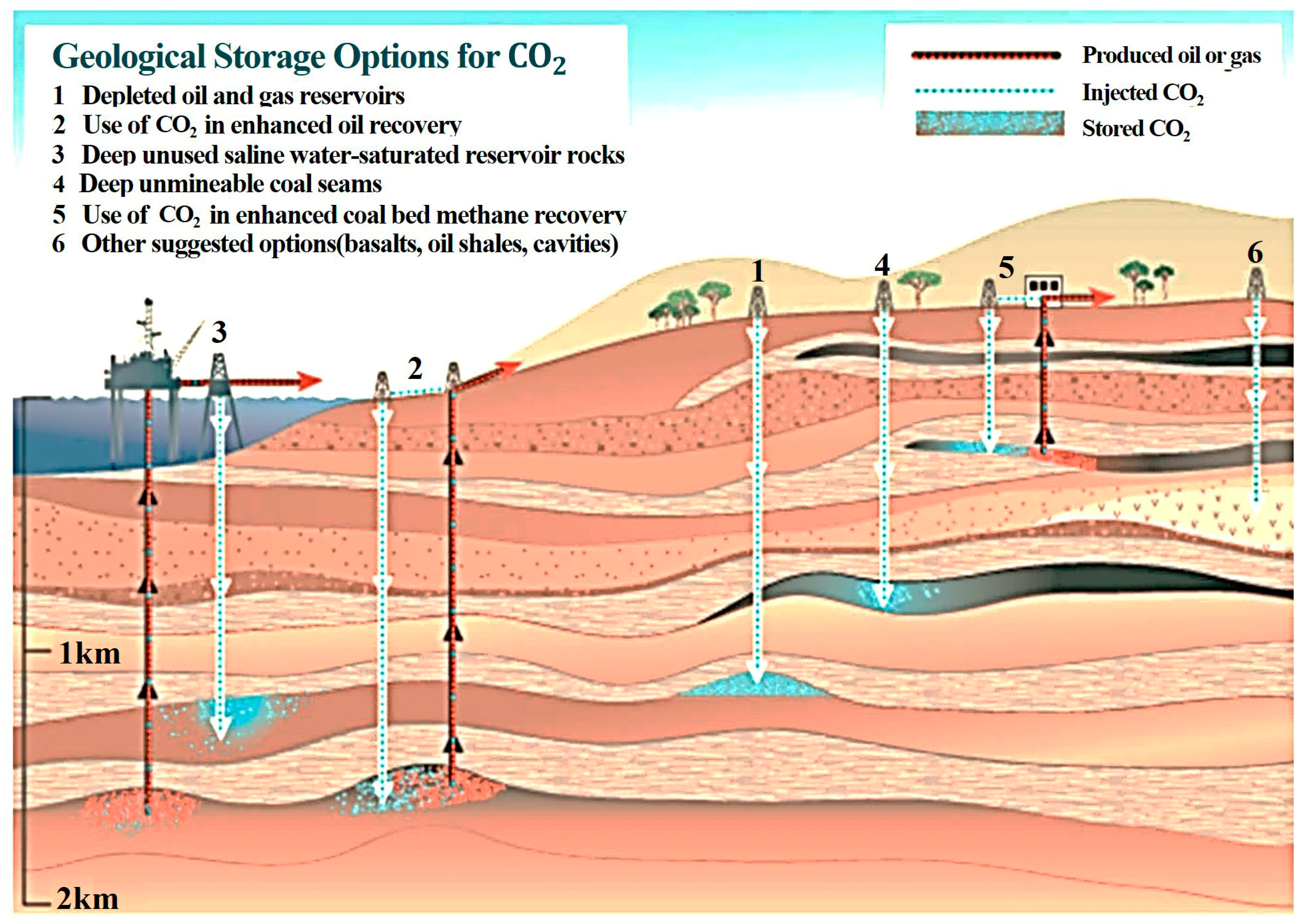
a.

Deep saline aquifers

Advantage: CO₂ storage in saline aquifers is widely regarded as one of the most practical settings for CGS due to the high potential storage capacity [23]. Additionally, the majority of these aquifers are currently unsuitable for other simultaneous or conflicting uses (though future use might include critical elements such as lithium), particularly in densely populated countries (Figure 2) [24].

Disadvantage: Many saline aquifers are currently unattractive for storage options due to the absence of required infrastructure, which is a significant economic drawback. This includes establishing injection wells, surface facilities, pipelines, and the substantial financial investments needed to establish such infrastructure [25].

b.

Depleted oil and gas reservoirs

Advantage: Extensive research conducted during hydrocarbon exploration makes it possible to assess storage capacity. Hydrocarbon-bearing formations demonstrate the long-term effectiveness of caprocks or seals, otherwise the oil and gas stored in them would have been depleted a significantly long time ago [26].

Disadvantage: The high concentration of oxygen in the carbon dioxide stream hampers the efficiency of CO₂-enhanced oil recovery (CO₂-EOR) processes. Excessive oxygen in the reservoir can enhance the growth of microorganisms [27]. This can eventually result in operational challenges, including injection blockage, oil degradation, and oil souring [28]. The environmental issues associated with enhanced oil recovery (EOR) encompass the production of large quantities of water, potentially contaminated with radioactive materials and harmful heavy metals [29].

c.

Unmineable coal seams

Advantage: Utilizing coal seams that cannot be mined offers an alternative solution for the storage of CO₂. The presence of cracks in the coal layer provides some permeability to the coal formation. Additionally, coal contains abundant tiny pores that can absorb large amounts of gas [30].

Disadvantage: Potential routes for CO₂ escape from sequestration in coal seam reservoirs include 1. inherent pathways such as faults and fractures; 2. inadequately cemented wellbores; 3. malfunction of wellbores or cap rock; and 4. dissolution of CO₂ in groundwater (Figure 2) [31].

d.

Basalt formations

Advantage: Constituting about 8% of the Earth’s continents and forming the majority of the oceanic crust, basalt provides significant potential as a storage reservoir for carbon dioxide [32]. These rocks possess the capacity for carbon dioxide sequestration, offering a notable advantage in their high reactivity and abundance of divalent metal ions. This reactivity enables them to immobilize carbon dioxide over extended geological time scales [33].

Disadvantage: The reliability of basalt formations for CO₂ sequestration is questioned due to the potential presence of fissures in the overlying caprock layers. These fractures might lead to CO₂ leakage. On the other hand, CO₂ migrating through these fissures could become mineralized, thereby being trapped within the formation before it can escape to the surface [34]. Therefore, it is critical to conduct comprehensive research to understand the interaction dynamics between CO₂ and basalt formations.

e.

Gas hydrate storage

Advantage: The subsurface sequestration of carbon dioxide in the form of hydrates represents a promising and innovative approach. This method seeks to trap carbon dioxide molecules within the molecular lattice of water (Figure 2) [35]. Rapid formation of carbon dioxide hydrates can occur in the presence of water under specific pressure and temperature conditions [36].

Disadvantage: Given that hydrates maintain stability solely under high pressures and at temperatures below 10 °C, their applicability is limited to certain geological settings. This encompasses shallower sediment layers beneath frigid waters and extensive permafrost areas, which may not always be proximal to significant CO₂ sources [37].

f.

Enhanced geothermal systems

Advantage: CO₂-driven enhanced geothermal systems (EGS) could provide dual-benefit subsurface engineering, removing CO₂ and providing geothermal energy (Figure 2) [38].

Disadvantage: In enhanced geothermal systems (EGS), employing water as the thermal conduction medium is marred by the unavoidable depletion of water resources during the circulation process. Such depletion is of significant concern, given the high value placed on water resources, leading to consequential financial implications [38].

Figure 2. Illustration of different methods for geological CO₂ sequestration [39,40,41,42].

Figure 2. Illustration of different methods for geological CO₂ sequestration [39,40,41,42].

Global commercial-scale integrated carbon capture and storage (CCS) projects are shown in Figure 3. A first challenge of geological storage of carbon dioxide is to select and optimize favorable areas for carbon dioxide storage [43]. The selection and optimization of areas for geological storage of CO₂ requires assessment of reservoir conditions, capping conditions, and safety [44,45,46,47,48]. The safety of geological carbon storage has long been a major concern and is largely influenced by several key factors, including injection pressure and the heterogeneity of fractures and caprocks [49,50]. In order to ensure long-term CO₂ sequestration, a sufficiently large basin and a caprock with good sealing capacity are necessary [51].

At pressures greater than 7.4 MPa and temperatures greater than 31 °C, conditions typical of geological storage, CO₂ will be in a supercritical phase. Supercritical CO₂ exhibits physical properties that fall between those of gas and liquid phases, having lower viscosity than the liquid phase and higher density than the gas phase. As a result, more CO₂ can be stored in the same volume [52,53].

Deep aquifers, typically regarded as confined, are considered viable for CO₂ sequestration and storage and are chosen for disposing of hazardous wastes [54,55,56,57]. Benson and Cole (2008) [54] specifically noted that aquifers deeper than 800 m, capped by thick, extensive aquitards, are appropriate for CO₂ sequestration. However, it is now recognized that leakage is a potential issue for many crucial aquifers globally, and the integrity of underground waste storage may be affected by the varying vertical permeability of confining layers [54,56,58]. Consequently, there exists a persistent risk of CO₂ leakage, underscoring the need for a deeper understanding of factors that contribute to leakage and how subsurface properties may evolve over time.

From this brief overview, we can see that leakage from fractures or faults, the distribution of the surrounding faults, and the high cost are likely the three most important unsolved issues for most geological CO₂ storage methods. Thus, in this paper, we focus on methods to measure and monitor caprock confinement (vertical leakage in the caprock) and fracture properties. In particular, we review how the water level in wells in leaky aquifers can be used to measure hydrogeological and fracture properties using the response of water level to tides—a minimally invasive, convenient, and continuous approach to quantifying these properties and any changes over time.

2. Evaluation of the Confinement of Caprocks

Caprocks, as defined by Fleury et al. (2010) [59] to be strata with low to very low permeability located above CO₂ storage formations, are essential in impeding CO₂ migration and reducing leakage from reservoirs. The evolution of their permeability is predominantly influenced by hydro-chemo-mechanical processes [60,61,62].

2.1. Research Progress in Evaluating the Confinement of Caprocks

The risk assessment methods for CO₂ geological storage were comprehensively reviewed by Bai et al. (2022) [63]. They analyzed the effects of caprock-to-reservoir thickness ratio, caprock thickness, lithology, and other factors on the low-permeability and high-speed leakages of caprock. Their analysis provided theoretical support for the selection of sites and stratigraphy as well as risk assessment of leakage for CGS projects.

Traditional approaches for evaluating aquifer confinement and hydraulic connections have predominantly relied on numerical simulations and isotope tracing methods. However, the absence of detailed physical parameters such as porosity, intrinsic and relative permeability, dispersivity, and chemical parameters from rock and fluid samples, mineral composition, and fluid chemistry may render numerical simulations subject to significant uncertainties [64,65]. This limitation has led to isotopic methods becoming a vital supplemental technique (Figure 4). The isotopic profile of water can occasionally trace its sources, and radiogenic isotopes can offer insights into water age and source, providing a clearer picture of the hydraulic interactions and geochemical processes occurring between aquifers over large areas. Currently, for dating deep aquifers, especially in sedimentary basins, traditional methods such as carbon-14 (¹⁴C) dating are preferred [66]. Yet, the age of deep groundwater often surpasses the effective range of ¹⁴C (1–40 × 10³ years). Additionally, particularly near potential faults, a single index might not suffice to discern the hydraulic connections between diverse water sources. In situations where the water sources or lithologies of adjacent aquifers are similar, the sensitivity of hydrogen and oxygen stable isotopes, along with standard tracers like strontium isotopes (⁸⁷Sr/⁸⁶Sr), might be inadequate for assessing hydraulic connections [67,68,69]. Hence, evaluations based on groundwater age, frequently nearing the ¹⁴C dating threshold, require additional validation. Cosmogenic isotopes, such as ³⁶Cl (half-life: 301 ka), though useful for older water, present challenges due to subsurface production [70]; similarly, cosmogenic ⁸¹Kr (half-life: 229 ka) is viable provided issues related to air contamination are addressed [71]. The utilization of multiple tracers is generally advantageous [72]. Emerging isotopic tracing methods involving elements such as lithium (δ⁷Li), boron (δ¹¹B), calcium (δ⁴⁴/⁴⁰Ca), magnesium (δ²⁶Mg), and uranium (²³⁴U/²³⁸U) are not yet widely employed for determining hydraulic connectivity between aquifers but have potential. Consequently, quantitative and in situ assessments of hydraulic connections in aquifers, particularly those used for CO₂ geological storage, as well as measurements of the age of deep groundwater, remain limited.

The calculation of vertical permeability and the assessment of aquifer confinement can be effectively conducted through analyzing water-level responses to barometric pressure fluctuations and tidal strains, as demonstrated in several studies [73,74,75,76,77]. Rojstaczer (1988) [73] developed a methodology to use water-level reactions to changes in barometric pressure that has been extensively utilized for determining both horizontal and vertical hydraulic parameters, as further explored in subsequent research [76,78]. The implementation of these models, which correlate water-level variations to external drivers, requires that certain parameters are known, such as storage coefficients for aquifers and aquitards. This requirement implies that the models are not entirely autonomous, though the influence of these pre-set parameters is often minimal. Moreover, the application of these models is contingent on the availability of barometric pressure data, an opportunity not uniformly present across groundwater observation stations.

In a recent advance, Wang et al. (2018) [74] developed a comprehensive analytical solution for the tidal response of borehole water levels in semi-confined aquifers, encompassing both horizontal and vertical flows within a leaky aquifer framework. This model, building upon the foundational work of Hantush and Jacob (1955) [79] for leaky and multilayered aquifers, has been applied in various studies, such as analyzing pressure changes due to water injection/extraction in boreholes and in determining hydraulic characteristics of both aquifers and aquitards [58,74,75,76,80]. However, the application of this model, particularly in the context of the semidiurnal M₂ tidal wave, has raised concerns regarding the independence and accuracy of the results [74,76,81]. Meanwhile, Zhang et al. (2021) [58] developed a new calculation method, combining both the M₂ and the O₁ tidal wave responses, to obtain the hydraulic parameters, which enabled the results to be more precise.

2.2. Nondestructive Onsite Exploration of Caprock Confinement from the Tidal Response of Water Level

Utilizing the tidal-response leaky aquifer model developed by Wang et al. (2018) [74], Zhang et al. (2021) carried out an extensive assessment of aquifer confinement within the vast North China Platform, covering an area of over 2.0 million square kilometers (Figure 5) [58]. This comprehensive study involved a range of wells, reaching depths of up to 3.4 km, and was primarily aimed at determining vertical permeability and barometric efficiency, assessing the effectiveness of caprocks in confinement, and examining the influence of significant seismic events, specifically the 2008 M_W 7.9 Wenchuan and 2011 M_W 9.1 Tohoku earthquakes, on aquifer confinement.

The wells included in this study all exceed a depth of 400 m, a criterion set to ensure that capillary effects on water hydraulics are negligible. Additionally, their locations, over 100 km from the coast, minimize the impact of oceanic tides on water-level changes. The North China Platform’s tectonic stability and the uniformity of its geological structures across different areas simplify the task of interpreting and comparing tidal responses from various wells.

The findings of these investigations, as shown in Figure 6, indicate that most of the aquifers under study exhibit leakage. Interestingly, this leakage shows no correlation with either the depth of the aquifers or the thickness of the overlying geological barriers, such as the caprock. A novel approach in this research involved employing both the semidiurnal M₂ (0.5175 days) and diurnal O₁ (1.076 days) tidal waves in the inversion analysis of aquifer parameters, thus providing additional independent constraints on the model parameters [58]. The study compares the results of vertical permeability with barometric efficiency (BE) metrics, as illustrated in Figure 7. The observed leakage prior to large earthquakes suggests that enhanced leakage is not a consequence of seismic activity but is due to inherent geological structures. Notably, wells with more confined characteristics, exhibiting lower vertical permeability K’, displayed higher BE coefficients, corroborating the hypothesis of vertical leakage (Figure 7) [58].

The barometric efficiency and barometric phase shift of water level were calculated from cross-spectral deconvolution of the barometric time series with the water-level time series [58,82]. The barometric response function (BRF) is defined as

$$BRF\left(\omega \right)=\frac{Y_{WB}\left(\omega \right)}{Y_{BB}\left(\omega \right)}$$

(1)

where Y_WB(ω) and Y_BB(ω) are the cross-spectra of the time series of water level and the barometric pressure and the auto-spectrum of the barometric pressure, respectively. The barometric efficiency (BE) and the phase shift are calculated from BRF(ω), respectively,

$$A^{BRF}\left(\omega \right)=\left|BRF\left(\omega \right)\right|$$

(2)

$${\theta }^{BRF}\left(\omega \right)=\mathit{arg}\left[BRF\left(\omega \right)\right]$$

(3)

where arg ($\tilde{k}$) is the argument of the complex number $\tilde{k}$.

Furthermore, Zhang et al. (2021) [58] conducted the first systematic assessment of the confinement of aquifers overlain by mudstones or shales. Their findings indicate that, despite the extremely low permeability of mudstone/shale formations serving as caprocks, a significant number of these aquifers exhibit considerable leakage prior to major seismic events.

As a result, the effectiveness of confining deep aquifers in the North China Platform appears to be less reliable than previously thought. This revelation implies that the storage of CO₂ in these deep aquifers requires a more cautious approach, accompanied by thorough and continuous monitoring.

2.3. Model and Calculation Methods

Equations governing the leaky model of Wang et al. (2018) (see Figure 8) [74] are

$${A^{\prime }}_{M2}/{A^{\prime }}_{O1}=abs\left(\frac{i{\omega }_{M2}S}{\left(i{\omega }_{M2}S+\frac{K^{\prime }}{b^{\prime }}\right)\xi }\right)/abs\left(\frac{i{\omega }_{O1}S}{\left(i{\omega }_{O1}{S}_{aqu}+\frac{K^{\prime }}{b^{\prime }}\right)\xi }\right)$$

(4)

$${\eta }_{M2}=\mathit{arg}\left(\frac{i{\omega }_{M2}S}{\left(i{\omega }_{M2}S+\frac{K^{\prime }}{b^{\prime }}\right)\xi }\right)$$

(5)

$${\eta }_{O1}=\mathit{arg}\left(\frac{i{\omega }_{O1}S}{\left(i{\omega }_{O1}S+\frac{K^{\prime }}{b^{\prime }}\right)\xi }\right)$$

(6)

where

$$\xi =1+{\left(\frac{r_c}{r_w}\right)}^2\frac{i\omega r_w}{2T\beta }\frac{K_0\left(\beta r_w\right)}{K_1\left(\beta r_w\right)}$$

(7)

$$\beta ={\left(\frac{K^{\prime }}{{Tb}^{\prime }}+\frac{i\omega S}{T}\right)}^{\frac{1}{2}}$$

(8)

and A’ represents the absolute amplitude ratio between water-level fluctuations and solid Earth tides, with η denoting the phase shift. The terms “abs” and “arg” refer to the magnitude and angle of complex numbers, respectively, ω is the circular frequency of the tidal wave, K’ is the vertical hydraulic conductivity of the caprock, T is the aquifer’s horizontal transmissivity, S is the aquifer’s storage coefficient, b’ denotes the thickness of the caprock, r_c is the casing radius, and r_w stands for the well radius. The subscripts M₂ and O₁ indicate the M₂ and O₁ tidal frequencies.

Consequently, three input parameters (A’_M2/A’_O1, η_M2, η_O1) are translated into three output parameters (S, T, K’), enhancing stability [58]. The least squares fitting process depends on initial test values of T, S, and K’ [58,69]; the lithologies of the aquifer and caprock, each with specific ranges for hydraulic parameters, set the boundary conditions for the fitting [83]. These processes are elaborated upon in Zhang-Wang et al. (2021) and Yang et al. (2021) [58,69]. Briefly, during the non-linear, least squares inversion (Fsolve, https://www.mathworks.com/help/optim/ug/fsolve.html), initial values function as constraints, ensuring that the derived S and T values align with the parameter ranges of the aquifer rocks, while K’—indicating the vertical leakage of the aquifer—remains positive.

3. Evaluation of the Distribution of Fractures in the Aquifer–Caprock System

The orientation and permeability of fractures significantly influence the movement of fluids (such as water, oil, and gas) and thermal energy within Earth’s crust, particularly in areas with crystalline basement and fine-grained sedimentary rocks where the matrix permeability is generally low [84,85,86,87]. It is important to note that permeability is not static, and changes can follow seismic events [88,89]. The manner in which fractures react to seismic waves from specific azimuths is influenced by fracture orientation [90,91]. Therefore, changes in permeability triggered by earthquakes could be contingent on the characteristics of these fractures.

The likelihood of CO₂ leakage is increased by the presence of faults and fractures. Unidentified faults or fractures are another key factor leading to the loss of caprock integrity and CO₂ leakage, and the impact of transmissive faults on caprock integrity requires further investigation. When the aquifer is confined well, capillary pressure prevents the upward migration of CO₂. However, earthquakes, injections, and other factors could change the structure of the caprock.

3.1. Research Progress in Evaluating the Distribution of Fractures in the Aquifer–Caprock System

Traditional methods for studying deep underground fissures require 3D and expensive active seismic imaging technologies, which can only detect large structures (several hundred meters in length). The low frequency and long wavelength of natural earthquake waves make it impossible to detect shallow fractures and faults in the crust. Developing new methods for detecting shallow features has been a pressing concern [92].

The directional characteristics of water-conducting fractures can be discerned through the use of monitoring wells that capture fluctuations in water levels produced by solid Earth tides [93]. Variations in pressure within these fractures are influenced by their orientation relative to the changing principal directions of tidal strain. Consequently, the phase and amplitude of water-level fluctuations can reveal apparent orientations of these fractures.

3.2. Nondestructive Characterization of Fracture Orientations from the Tidal Response of Water Level

Changes in water level caused by the lunar tide (O₁) and semidiurnal tide (M₂) can provide a convenient, economical, and accurate method for detecting fissures that play a dominant role in fluid flow.

Zhang-Manga et al. (2022) [92] utilized a model that integrates the tidal response of fractures to the O₁ and M₂ tidal components for the calculation of fracture orientations (strikes and dips) within aquifer–caprock systems. The study employed the sign of the phase shift and magnitude of the amplitude ratio of the M₂ and O₁ tides in five wells situated on the North China platform, as illustrated in Figure 9 [92].

Following two significant regional earthquakes, alterations in the phase shift between tidal strain and water-level responses were observed in a number of these wells (Figure 10). These post-earthquake changes were initially ascribed to modifications in aquifer confinement [58], based on a model addressing vertical leakage through confining aquitards [74]. However, Zhang-Manga et al. (2022) [92] reassessed these earthquake responses using a different model that posits tidal responses as being governed by conductive fractures intersecting the wells, a concept initially proposed by Hanson and Owen (1982) [93].

Zhang-Manga et al. (2022) [92] conducted calculations to determine the orientation (strike and dip) of fractures and assessed the effects of significant earthquakes (2008 M_W 7.9 Wenchuan and 2011 M_W 9.1 Tohoku) on these fractures. Their analysis indicated that the fracture orientations in deep wells (ranging from 400 m to 3500 m) predominantly align east–west (Figure 11), mirroring the regional faults and stress patterns (Figure 9). They also observed that seismic waves from the distant Wenchuan earthquake (over 1000 km from the epicenter) and the Tohoku earthquake (more than 2000 km from the epicenter) could alter the apparent orientation of the fractures (Figure 11). Among the four groundwater wells impacted by seismic wave energy densities nearing or exceeding 0.1 J/m³, the orientation of fractures in three wells exhibited significant shifts post-earthquake, whereas one well showed no change (Figure 11). This suggests varying sensitivities of geological formations to seismic activity. The energy density of the 2008 M_W 7.9 Wenchuan earthquake was generally lower compared to the 2011 M_W 9.1 Tohoku earthquake. Nonetheless, the orientation of fractures in five wells altered (three significantly), possibly due to the higher frequency of seismic waves from the Wenchuan earthquake. Therefore, the alteration in apparent fracture orientation might be influenced not just by energy density but also by the frequency of seismic waves. The extent to which seismic wave frequency affects hydrogeological properties is still a topic of ongoing investigation and uncertainty [94].

Given the minimal stress exerted by distant seismic waves, it is highly improbable that seismic waves directly lead to the formation of new fractures. More plausible is that the fluid flow oscillations caused by seismic waves alter the interconnectivity and apparent orientation of existing fractures (Figure 12) by either clearing or obstructing pre-existing flow channels [92]. The process of fracture unclogging is frequently cited as a mechanism for permeability variations due to dynamic stresses: this phenomenon has been observed in laboratory settings [95,96,97,98], field studies [77,99,100,101,102,103,104], and numerical simulations [105], potentially leading to shifts in the apparent direction of hydraulically conductive fractures.

The orientation of fractures could be impacted not only by large earthquakes but also by anthropogenic disturbances. Although the pre-earthquake orientation in 2011 (Figure 11b) is not the same as post-earthquake orientation in 2008 (Figure 11a), the values are similar. For some wells, the re-orientation induced by earthquakes persists for a short time span after the earthquake, while for other wells, it could be permanent [106].

3.3. Model and Calculation Methods

The tidal strain fracture orientation technique was initially developed by Hanson and Owen (1982) [93]. They solved for the amplitudes and phases of O₁ and M₂ tides in the time series of fluid pressure. These solutions are functions of the strike and dip of either a single highly conductive fracture or a set of parallel fractures intersecting the wellbore.

In this framework, let $\widehat{\mathrm{n}}$ represent the normal vector to the fracture plane. This is defined by direction cosines as $\hat{\mathrm{n}}=\left(\cos {\alpha }_1,\cos {\alpha }_2,\cos {\alpha }_3\right)$, where α₁, α₂, and α₃ are the angles between $\widehat{\mathrm{n}}$ and the east, north, and vertical directions, respectively, as detailed by Barbour et al. (2019) [107]. A time-varying tidal strain tensor $\xi (t)$ will produce strain normal to the fracture plane of $\delta (t)=\hat{\mathrm{n}}\xi (t){\hat{\mathrm{n}}}^{\mathrm{T}}$. Consequently, the fluid pressure response in the fracture will be

$$p\left(t\right)=-Q\hat{\mathrm{n}}\xi \left(t\right){\hat{\mathrm{n}}}^{\mathrm{T}}$$

(9)

The proportionality constant Q (positive) depends on elastic parameters of the host rock, fracture size, wellbore storage effects, and fluid compressibility. The tidal strain tensor in the frequency domain is

$$\tilde{\xi }\left({\omega }_Q\right)=\left[\begin{array}{ccc}{\tilde{\xi }}_{\lambda \lambda }\left({\omega }_Q\right)& \frac{1}{2}{\tilde{\xi }}_{\lambda \theta }\left({\omega }_Q\right)& 0\\ \frac{1}{2}{\tilde{\xi }}_{\lambda \theta }\left({\omega }_Q\right)& {\tilde{\xi }}_{\theta \theta }\left({\omega }_Q\right)& 0\\ 0& 0& {\tilde{\xi }}_{zz}\left({\omega }_Q\right)\end{array}\right]$$

(10)

where λ is longitude (positive east), θ is latitude (positive north), and ω_Q is the frequency. When loading by tidal water bodies can be neglected, ${\tilde{\xi }}_{\lambda \lambda }({\omega }_Q)$ and ${\tilde{\xi }}_{\theta \theta }({\omega }_Q)$ are in phase with the tidal potential and ${\tilde{\xi }}_{\lambda \theta }({\omega }_Q)$ leads (diurnal constituents) or lags (semidiurnal constituents) the tidal potential by 90°, and

$$\begin{array}{ll}\hfill & \tilde{p}\left({\omega }_Q\right)=\frac{Qv}{1-v\left[\left|{\tilde{\xi }}_{\theta \theta }\left({\omega }_Q\right)\right|+\left|{\tilde{\xi }}_{\lambda \lambda }\left({\omega }_Q\right)\right|\right]\exp \left(i{\varphi }_Q\right)}\hfill \\ \hfill & -\frac{Q}{1-v\left[\left|{\tilde{\xi }}_{\lambda \lambda }\left({\omega }_Q\right)\right|+v\left|{\tilde{\xi }}_{\theta \theta }\left({\omega }_Q\right)\right|\right]\exp \left(i{\varphi }_Q\right){\cos }^2{\alpha }_1}\hfill \\ \hfill & -\frac{Q}{1-v\left[\left|{\tilde{\xi }}_{\theta \theta }\left({\omega }_Q\right)\right|+v\left|{\tilde{\xi }}_{\lambda \lambda }\left({\omega }_Q\right)\right|\right]\exp \left(i{\varphi }_Q\right){\cos }^2{\alpha }_2}\hfill \\ \hfill & \mp iQ\left|{\tilde{\xi }}_{\lambda \theta }\left({\omega }_Q\right)\right|\exp \left(i{\varphi }_Q\right)\cos {\alpha }_1\cos {\alpha }_2\hfill \end{array}$$

(11)

The phase, relative to the tidal potential, of the pressure change for the kth constituent can be obtained using

$$\begin{array}{ll}\hfill & \tan \left(\mathrm{Arg}\left\{\tilde{p}\left({\omega }_Q\right)\exp \left(-i{\varphi }_Q\right)\right\}\right)=\hfill \\ \hfill & \frac{\mp \left(1-v\right)\left|{\tilde{\xi }}_{\lambda \theta }\left({\omega }_Q\right)\right|\cos {\alpha }_1\cos {\alpha }_2}{v\left[\left|{\tilde{\xi }}_{\theta \theta }\left({\omega }_Q\right)\right|+\left|{\tilde{\xi }}_{\lambda \lambda }\left({\omega }_Q\right)\right|\right]-\left[{\tilde{\xi }}_{\lambda \lambda }\left({\omega }_Q\right)\left|+v\right|{\tilde{\xi }}_{\theta \theta }\left({\omega }_Q\right)\mid \right]{\cos }^2{\alpha }_1-\left[{\tilde{\xi }}_{\theta \theta }\left({\omega }_Q\right)\left|+v\right|{\tilde{\xi }}_{\lambda \lambda }\left({\omega }_Q\right)\mid \right]{\cos }^2{\alpha }_2}\hfill \end{array}$$

(12)

where the + is used for M₂ tides and − is used for O₁ tides. The ratio of the amplitudes for two frequencies ω_k and ω_j is

$$\frac{\left|\tilde{p}\left({\omega }_k\right)\right|}{\left|\tilde{p}\left({\omega }_j\right)\right|}={\left[\frac{\Re {\left[\tilde{p}\left({\omega }_k\right)\right]}^2+\Im {\left[\tilde{p}\left({\omega }_k\right)\right]}^2}{\Re {\left[\tilde{p}\left({\omega }_j\right)\right]}^2+\Im {\left[\tilde{p}\left({\omega }_j\right)\right]}^2}\right]}^{\frac{1}{2}}=\mathrm{Mod}\left\{\frac{\tilde{p}\left({\omega }_k\right)}{\tilde{p}\left({\omega }_j\right)}\right\}$$

(13)

Equations (12) and (13), which are independent of Q, were used to search for fracture strikes and dips that yielded amplitude ratios and phases in agreement with the observed tidal amplitudes and phases. In addition,

$${\cos }^2{\alpha }_1+{\cos }^2{\alpha }_2+{\cos }^2{\alpha }_3=1$$

(14)

The known variables include the amplitudes and phases of the M₂ and O₁ constituents in the solid Earth strain tides. These are calculated using the Mapsis package [108] for each well’s location, as illustrated in Figure 9. Hence, to determine the fracture orientation (dip and strike, inferred from α₁, α₂, α₃), the set of N equations is solved as a nonlinear least squares problem, utilizing the amplitudes and phases of body strain tides at the well locations [92].

4. Effects of Shale-Induced Heterogeneity and Anisotropy on Tidal Response of Water Level

While tidal response models to interpret water-level variations are extensively utilized [73,74,76,77], the impact of heterogeneity in these models, particularly the effects of low-permeability, low-porosity, and anisotropic shale layers, have been mostly overlooked. Shale formations, due to their low porosity and permeability (ranging from 10⁻⁴ to 10⁻³ mD), as well as their interaction with high-porosity and high-permeability surrounding rocks, lead to anisotropic and heterogeneous geological formations. Therefore, aquifers containing shale may show distinctive features [62]. Since most wells are drilled and screened in permeable formations, groundwater wells are typically biased away from containing shale, and few studies have addressed this topic. However, many theoretical analytical models in hydrogeology, such as the barometric-response leaky aquifer model and the tidal-response leaky aquifer model, assume that the rock formations are homogeneous and isotropic, leading to differences between theoretical models and actual conditions and, hence, errors in computed hydrogeological properties [62].

The influence of shale interlayers within aquifers (e.g., Figure 13) on the tidal-response leaky aquifer model, as proposed by Wang et al. (2018) [74], was investigated by Zhang et al. (2023) [62]. Their analyses and comparative studies suggest that wells with minor amounts of shale (exceeding approximately 5%) in the aquifer’s screened segment can lead to pronounced anisotropy and heterogeneity and, as a result, deviations from the ideal analytical solution of the tidal-response leaky aquifer model [74]. Consequently, this model may only offer approximate estimates.

The large deviation in the phase shift for the O₁ wave in the HZ well (Figure 14) is due to the inversion of an excessively flat phase shift (Figure 14 red dots), which is attributed to the unconstrained analytical solution [58]. The vertical permeability coefficient K’ of the HZ well is close to 0 (corresponding to a value of 10⁻¹⁰ m/s). With reference to the analytical solution, K’ becomes “flat” and is no longer sensitive to model parameters when K’ < 10⁻⁷ m/s [58].

Wang et al. (2018) [74] noted that in the tidal-response leaky model, phase shifts are markedly more responsive to permeability changes than amplitude ratios, which was the focus of their analysis. Similarly, Zhang et al. (2021) [58] also concentrated on calculating the phase shift. The degree of phase shift deviation increases with increasing shale content within the aquifer (Figure 15 and Figure 16).

These conclusions were further confirmed through COMSOL numerical simulations (Figure 16). Therefore, in aquifers containing shale, using idealized isotropic and homogeneous models (such as the tidal- and barometric-response leaky aquifer models) can only yield approximate estimates. To avoid data quality issues caused by heterogeneity and anisotropy (such as unstable flow resulting from local pore pressure excess), it is advisable to avoid interpreting data from wells screened near layers of shale.

5. Approximations and Application Limitations in Tidal Response Models

5.1. Idealizations in the Tidal-Response Leaky Aquifer Model

The tidal-response leaky aquifer model is a one-dimensional model with vertical flow in the confining layer and horizontal flow in the aquifer (Figure 8). Further idealizations include the assumption of a homogeneous and isotropic aquifer and aquitard, that aquitard storage is negligible, no basement leakage, periodic discharge of the well will not impact the water table, and the well is a line source [92]. Some wells do not satisfy these approximations, especially the isotropic and homogenous assumptions, and, thus, the model yields rough estimates of properties [92].

5.2. Idealizations in the Tidal-Response Fracture Model

The model developed by Hanson and Owen (1982) [93] is for a single fracture with sufficiently high permeability such that the well senses the change in pressure in the fracture as tidal strains compress and dilate the fracture. Thus, wells intersecting fractures with relatively low fracture permeability could deviate from the solutions obtained from this model [106]. In the context of applying the model to an actual aquifer that may intersect multiple, non-planar fractures and a permeable host aquifer, the best-fit strikes and dips should be interpreted as an average of the hydraulically transmissive fractures that intersect the well that is equivalent to a single most transmissive feature [106].

6. Conclusions, Outlook, and Recommendations

Deformation of the subsurface by external forcings, such as barometric pressure variations at the Earth’s surface or volumetric strains from solid Earth tides, provide an opportunity to measure and monitor properties of subsurface formations including permeability, storage, aquifer leakage, and fracture orientations. However, interpretations can be non-unique and the same observations that suggest that aquifers are leaky can be explained by strains in fractures. The use of multiple forcings and multiple frequencies of tides, such as both the M₂ and O₁ tidal waves [58,92], can help reduce some of the non-uniqueness in determining properties of the subsurface and their changes over time. Recent studies have also highlighted that some of the idealizations in subsurface flow models, such as homogeneity of aquifers and low permeabilities, can lead to inaccurate results when models are applied to data.

Long-term monitoring of deep groundwater has revealed that hydrogeological properties are not constant and can be impacted by the small strains from distant earthquakes. Subsurface changes can be large enough for reservoirs to become leaky. We, thus strongly support construction of monitoring wells, or monitoring existing wells, in regions where CO₂ is disposed in the subsurface. Further, monitoring a range of formations and at a high enough sampling frequency to enable tidal analysis are important in providing a broad perspective on where, when, and why properties of the subsurface change.

References

- He, H.; Lian, J.; Chen, C.; Xiong, Q.; Li, C.C.; Zhang, M. Enabling Multi-Chemisorption Sites on Carbon Nanofibers Cathodes by an In-situ Exfoliation Strategy for High-Performance Zn–Ion Hybrid Capacitors. Nano-Micro Lett. 2022, 14, 106. [Google Scholar] [CrossRef]
- Zhao, Y.; Setzler, B.P.; Wang, J.; Nash, J.; Wang, T.; Xu, B.; Yan, Y. An Efficient Direct Ammonia Fuel Cell for Affordable Carbon-Neutral Transportation. Joule 2019, 3, 2472–2484. [Google Scholar] [CrossRef]
- Cao, C.; Liu, H.; Hou, Z.; Mehmood, F.; Liao, J.; Feng, W. A Review of CO2 Storage in View of Safety and Cost-Effectiveness. Energies 2020, 13, 600. [Google Scholar] [CrossRef]
- IEA. CO2 Emissions from Fuel Combustion—Highlights; IEA: Paris, France, 2016. [Google Scholar]
- NASA—National Aeronautics and Space Administration. Carbon Dioxide. 2017. Available online: https://climate.nasa.gov/vital-signs/carbon-dioxide/ (accessed on 10 August 2017).
- Met-Office. Global Climate in Context as the World Approaches 1 °C above Preindustrial for the First Time. 2015. Available online: http://www.metoffice.gov.uk/research/news/2015/global-average-temperature-2015 (accessed on 15 August 2022).
- IPCC. Special Report on Carbon Dioxide Capture and Storage; IPCC: Cambridge, UK, 2005. [Google Scholar]
- ECF. Roadmap 2050. A Practical Guide to a Prosperous, Low-Carbon Europe; ECF: Brussels, Belgium, 2010. [Google Scholar]
- IEA. CO2 Emissions from Fuel Combustion 2009; OECD Publishing: Paris, France, 2009. [Google Scholar]
- Viebahn, P.; Vallentin, D.; Höller, S. Prospects of carbon capture and storage (CCS) in China’s power sector—An integrated assessment. Appl. Energy 2015, 157, 229–244. [Google Scholar] [CrossRef]
- Kumar, S.; Foroozesh, J.; Edlmann, K.; Rezk, M.G.; Lim, C.Y. A comprehensive review of value-added CO2 sequestration in subsurface saline aquifers. J. Nat. Gas Sci. Eng. 2020, 81, 103437. [Google Scholar] [CrossRef]
- Aminu, M.D.; Nabavi, S.A.; Rochelle, C.A.; Manovic, V. A review of developments in carbon dioxide storage. Appl. Energy 2017, 208, 1389–1419. [Google Scholar] [CrossRef]
- Ajayi, T.; Gomes, J.S.; Bera, A. A review of CO2 storage in geological formations emphasizing modeling, monitoring and capacity estimation approaches. Pet. Sci. 2019, 16, 1028–1063. [Google Scholar] [CrossRef]
- Zhou, N.; Lu, S.; Wang, M.; Liu, W.; Guan, Y.; Tan, H.; Wang, Z. Applicability of fractal capillary pressure models to sandstones. J. Pet. Sci. Eng. 2020, 185, 106626. [Google Scholar] [CrossRef]
- Kalam, S.; Olayiwola, T.; Al-Rubaii, M.M.; Amaechi, B.I.; Jamal, M.S.; Awotunde, A.A. Carbon dioxide sequestration in underground formations: Review of experimental, modeling, and field studies. J. Pet. Explor. Prod. Technol. 2021, 11, 303–325. [Google Scholar] [CrossRef]
- Khudaida, K.J.; Das, D.B. A numerical study of capillary pressure–saturation relationship for supercritical carbon dioxide (CO2) injection in deep saline aquifer. Chem. Eng. Res. Des. 2014, 92, 3017–3030. [Google Scholar] [CrossRef][Green Version]
- Song, J.; Zhang, D. Comprehensive Review of Caprock-Sealing Mechanisms for Geologic Carbon Sequestration. Environ. Sci. Technol. 2013, 47, 9–22. [Google Scholar] [CrossRef]
- Jiao, Z.; Pawar, R.; Duguid, A.; Bourcier, W.; Haussmann, C.; Coddington, K.; Harp, D.; Ganshin, Y.; Quillinan, S.; Mclaughlin, F.; et al. A Field Demonstration of an Active Reservoir Pressure Management through Fluid Injection and Displaced Fluid Extraction at the Rock Springs Uplift a Priority Geologic CO2 Storage Site for Wyoming. Energy Procedia 2017, 114, 2799–2811. [Google Scholar] [CrossRef]
- Das, D.B.; Mirzaei, M.; Widdows, N. Non-uniqueness in capillary pressure–saturation–relative permeability relationships for two-phase flow in porous media: Interplay between intensity and distribution of random micro-heterogeneities. Chem. Eng. Sci. 2006, 61, 6786–6803. [Google Scholar] [CrossRef][Green Version]
- Celia, M.A.; Bachu, S.; Nordbotten, J.M.; Bandilla, K.W. Status of CO2 storage in deep saline aquifers with emphasis on modeling approaches and practical simulations. Water Resour. Res. 2015, 51, 6846–6892. [Google Scholar] [CrossRef]
- Bachu, S. Screening and ranking of sedimentary basins for sequestration of CO2 in geological media in response to climate change. Environ. Geol. 2003, 44, 277–289. [Google Scholar] [CrossRef]
- Eigbe, P.A.; Ajayi, O.O.; Olakoyejo, O.T.; Fadipe, O.L.; Efe, S.; Adelaja, A.O. A general review of CO2 sequestration in underground geological formations and assessment of depleted hydrocarbon reservoirs in the Niger Delta. Appl. Energy 2023, 350, 121723. [Google Scholar] [CrossRef]
- Bachu, S. Sequestration of CO2 in geological media: Criteria and approach for site selection in response to climate change. Energy Convers Manag. 2000, 41, 953–970. [Google Scholar] [CrossRef]
- Trémosa, J.; Castillo, C.; Vong, C.Q.; Kervévan, C.; Lassin, A.; Audigane, P. Long-term assessment of geochemical reactivity of CO2 storage in highly saline aquifers: Application to Ketzin, In Salah and Snøhvit storage sites. Int. J. Greenh. Gas Control 2014, 20, 2–26. [Google Scholar] [CrossRef]
- Li, Z.; Dong, M.; Li, S.; Huang, S. CO2 sequestration in depleted oil and gas reservoirs—Caprock characterization and storage capacity. Energy Convers. Manag. 2006, 47, 1372–1382. [Google Scholar] [CrossRef]
- Heinemann, N.; Wilkinson, M.; Pickup, G.E.; Haszeldine, R.S.; Cutler, N.A. CO2 storage in the offshore UK Bunter Sandstone formation. Int. J. Greenh. Gas Control 2012, 6, 210–219. [Google Scholar] [CrossRef]
- Porter, R.T.J.; Fairweather, M.; Pourkashanian, M.; Woolley, R.M. The range and level of impurities in CO2 streams from different carbon capture sources. Int. J. Greenh. Gas Control 2015, 36, 161–174. [Google Scholar] [CrossRef]
- Morgan, H.; Large, D.; Bateman, K.; Hanstock, D.; Gregory, S. The Effect of Variable Oxygen Impurities on Microbial Activity in Conditions Resembling Geological Storage Sites. Energy Procedia 2017, 114, 3077–3087. [Google Scholar] [CrossRef]
- Igunnu, E.T.; Chen, G.Z. Produced water treatment technologies. Int. J. Low-Carbon Technol. 2014, 9, 157. [Google Scholar] [CrossRef]
- Shukla, R.; Ranjith, P.; Haque, A.; Choi, X. A review of studies on CO2 sequestration and caprock integrity. Fuel 2010, 89, 2651–2664. [Google Scholar] [CrossRef]
- Shi, J.Q.; Durucan, S. CO2 Storage in Deep Unminable Coal Seams. Oil Gas Sci. Technol. Rev. D’ifp Energ. Nouv. 2005, 60, 547–558. [Google Scholar] [CrossRef]
- Gíslason, S.R.; Broecker, W.S.; Gunnlaugsson, E.; Snæbjörnsdóttir, S.Ó.; Mesfin, K.G.; Alfredsson, H.A.; Aradóttir, E.S.; Sigfússon, B.; Gunnarsson, I.; Stute, M.; et al. Rapid solubility and mineral storage of CO2 in basalt. Energy Procedia 2014, 63, 4561–4574. [Google Scholar] [CrossRef]
- Van Pham, T.H.; Aagaard, P.; Hellevang, H. On the potential for CO2 mineral storage in continental flood basalts-PHREEQC batch- and 1D diffusion-reaction simulations. Geochem. Trans. 2012, 13, 5. [Google Scholar] [CrossRef] [PubMed]
- IEAGHG. Geological Storage of CO2 in Basalts; IEAGHG: Cheltenham, UK, 2011. [Google Scholar]
- Yang, H.; Xu, Z.; Fan, M.; Gupta, R.; Slimane, R.B.; Bland, A.E.; Wright, I.G. Progress in carbon dioxide separation and capture: A review. J. Environ. Sci. 2008, 20, 14–27. [Google Scholar] [CrossRef]
- Circone, S.; Stern, L.A.; Kirby, S.H.; Durham, W.B.; Chakoumakos, B.C.; Rawn, C.J.; Rondinone, A.J.; Ishii, Y. CO2 hydrate: Synthesis, composition, structure, dissociation behavior, and a comparison to structure I CH4 hydrate. J. Phys. Chem. B 2003, 107, 5529–5539. [Google Scholar] [CrossRef]
- Singh, R.P.; Shekhawat, K.S.; Das, M.K.; Muralidhar, K. Geological sequestration of CO2 in a water-bearing reservoir in hydrate-forming conditions. Oil Gas Sci. Technol. Rev. IFP Energ. Nouv. 2020, 75, 51. [Google Scholar] [CrossRef]
- Pruess, K. Enhanced geothermal systems (EGS) using CO2 as working fluid—A novel approach for generating renewable energy with simultaneous sequestration of carbon. Geothermics 2006, 35, 351–367. [Google Scholar] [CrossRef]
- Zhao, X.; Liao, X.; Wang, W.; Chen, C.; Rui, Z.; Wang, H. The CO2 storage capacity evaluation: Methodology and determination of key factors. J. Energy Inst. 2014, 87, 297–305. [Google Scholar] [CrossRef]
- Mazzotti, M.; Pini, R.; Storti, G.; Burlini, L. Carbon dioxide (CO2) sequestration in unmineable coal seams and use for enhanced coalbed methane recovery (ECBM). In Developments and Innovation in Carbon Dioxide (CO2) Capture and Storage Technology; Elsevier: Amsterdam, The Netherlands, 2010; pp. 127–165. [Google Scholar] [CrossRef]
- Rochelle, C.A.; Camps, A.P.; Long, D.; Milodowski, A.; Bateman, K.; Gunn, D.; Jackson, P.; Lovell, M.A.; Rees, J. Can CO2 hydrate assist in the underground storage of carbon dioxide? Geol. Soc. Spec. Publ. 2009, 319, 171–183. [Google Scholar] [CrossRef]
- Bui, M.; Adjiman, C.S.; Bardow, A.; Boston, A.; Brown, S.F.; Fennell, P.S.; Fuss, S.; Galindo, A.; Hackett, L.A.; Hallett, J.P.; et al. Carbon capture and storage (CCS): The way forward. Energy Environ. Sci. 2018, 11, 1062–1176. [Google Scholar] [CrossRef]
- Lu, P.; Hao, Y.; Bai, Y.; Liu, W.; Chen, X.; Zheng, H.; Liu, J.; Chen, Y.; Gao, J.-P. Optimal selection of favorable areas for CO2 geological storage in the Majiagou Formation in the Ordos Basin. Int. J. Greenh. Gas Control 2021, 109, 103360. [Google Scholar] [CrossRef]
- Surdam, R.C.; Jiao, Z.; Ganshin, Y.; Bentley, R.D.; García-González, M.; Quillinan, S.A.; Mclaughlin, J.F.; Stauffer, P.H.; Deng, H. Characterizations of the CCUS Attributes of a High-priority CO2 Storage Site in Wyoming, USA. Energy Procedia 2013, 37, 3911–3918. [Google Scholar] [CrossRef][Green Version]
- Wang, X.; Zhang, D.; Su, E.; Jiang, Z.; Wang, C.; Chu, Y.; Ye, C. Pore structure and diffusion characteristics of intact and tectonic coals: Implications for selection of CO2 geological sequestration site. J. Nat. Gas Sci. Eng. 2020, 81, 103388. [Google Scholar] [CrossRef]
- Lu, J.; Mickler, P.J.; Nicot, J.; Yang, C.; Darvari, R. Geochemical impact of O2 impurity in CO2 stream on carbonate carbon-storage reservoirs. Int. J. Greenh. Gas Control 2016, 47, 159–175. [Google Scholar] [CrossRef]
- Blackford, J.; Alendal, G.; Avlesen, H.; Brereton, A.; Cazenave, P.W.; Chen, B.; Dewar, M.; Holt, J.T.; Phelps, J.J. Impact and detectability of hypothetical CCS offshore seep scenarios as an aid to storage assurance and risk assessment. Int. J. Greenh. Gas Control 2020, 95, 102949. [Google Scholar] [CrossRef]
- Park, J.; Lee, S.; Kihm, J.; Kim, J.; Lee, Y.I. Probabilistic evaluation of multi-fluid-phase carbon dioxide storage capacities of saline formations in the Pohang Basin, Korea using three-dimensional geologic modeling and grid-based Monte Carlo simulation. Int. J. Greenh. Gas Control 2018, 79, 289–312. [Google Scholar] [CrossRef]
- Li, Q.; Han, Y.; Liu, X.; Ansari, U.; Cheng, Y.; Yan, C. Hydrate as a by-product in CO2 leakage during the long-term sub-seabed sequestration and its role in preventing further leakage. Environ. Sci. Pollut. Res. 2022, 29, 77737–77754. [Google Scholar] [CrossRef]
- Li, Q.; Wang, F.; Wang, Y.; Forson, K.; Cao, L.; Zhang, C.; Zhou, C.; Zhao, B.; Chen, J. Experimental investigation on the high-pressure sand suspension and adsorption capacity of guar gum fracturing fluid in low-permeability shale reservoirs: Factor analysis and mechanism disclosure. Environ. Sci. Pollut. Res. 2022, 29, 53050–53062. [Google Scholar] [CrossRef]
- Armitage, P.J.; Worden, R.H.; Faulkner, D.; Aplin, A.C.; Butcher, A.R.; Espie, A.A. Mercia Mudstone Formation caprock to carbon capture and storage sites: Petrology and petrophysical characteristics. J. Geol. Soc. 2013, 170, 119–132. [Google Scholar] [CrossRef]
- Lee, Y.; Kim, K.; Sung, W.; Yoo, I. Analysis of the Leakage Possibility of Injected CO2 in a Saline Aquifer. Energy Fuels 2010, 24, 3292–3298. [Google Scholar] [CrossRef]
- Zhang, K.; Xie, J.; Li, C.; Hu, L.; Wu, X.; Wang, Y. A full chain CCS demonstration project in northeast Ordos Basin, China: Operational experience and challenges. Int. J. Greenh. Gas Control 2016, 50, 218–230. [Google Scholar] [CrossRef]
- Benson, S.M.; Cole, D.R. CO2 sequestration in deep sedimentary formations. Elements 2008, 4, 325–331. [Google Scholar] [CrossRef]
- Weingarten, M.; Ge, S.; Godt, J.W.; Bekins, B.A.; Rubinstein, J.L. High-rate injection is associated with the increase in U.S. mid-continent seismicity. Science 2015, 348, 1336–1340. [Google Scholar] [CrossRef]
- U.S. Environmental Protection Agency. Hydraulic Fracturing for Oil and Gas: Impacts from the Hydraulic Fracturing Water Cycle on Drinking Water Resources in the United States; U.S. Environmental Protection Agency: Washington, DC, USA, 2016; Volume 81, pp. 95135–95136.
- Walsh, F.R.; Zoback, M.D. Oklahoma’s recent earthquakes and saltwater disposal. Sci. Adv. 2015, 1, e1500195. [Google Scholar] [CrossRef] [PubMed]
- Zhang, Y.; Wang, C.Y.; Fu, L.Y.; Yang, Q.Y. Are deep aquifers really confined? Insights from deep groundwater tidal responses in the North China Platform. Water Resour. Res. 2021, 57, e2021WR030195. [Google Scholar] [CrossRef]
- Fleury, M.; Pironon, J.; Nindre, Y.M.; Bildstein, O.; Berne, P.; Lagneau, V.; Broseta, D.; Pichery, T.; Fillacier, S.; Lescanne, M.; et al. Evaluating Sealing Efficiency of Caprocks for CO2 Storage: An Overview of the Geocarbone-Integrity Program and Results. Oil Gas Sci. Technol. Rev. De L’institut Français Du Pétrole 2010, 65, 435–444. [Google Scholar] [CrossRef][Green Version]
- Anyim, K.; Gan, Q. Fault zone exploitation in geothermal reservoirs: Production optimization, permeability evolution and induced seismicity. Adv. Geo-Energy Res. 2020, 4, 1–12. [Google Scholar] [CrossRef]
- Cai, J.; Wei, W.; Hu, X.; Liu, R.; Wang, J. Fractal characterization of dynamic fracture network extension in porous media. Fractals 2017, 25, 1750023. [Google Scholar] [CrossRef]
- Zhang, Y.; Fu, L.-Y.; Zhu, A.; Zhao, L.; Qi, S.; Huang, T.; Ma, Y.C.; Zhang, W. Anisotropy and heterogeneity induced by shale in aquifer lithology—Influence of aquifer shale on the leaky model with tidal response analysis. Water Resour. Res. 2023, 59, e2021WR031451. [Google Scholar] [CrossRef]
- Bai, M.; Zhang, Z.; Bai, H.; Du, S. Progress in Leakage Risk Study of CO2 Geosequestration System. Spec. Oil Gas Reserv. 2022, 29, 1–11. [Google Scholar]
- Vilarrasa, V.; Bolster, D.; Olivella, S.; Carrera, J. Coupled hydromechanical modeling of CO2 sequestration in deep saline aquifers. Int. J. Greenh. Gas Control 2010, 4, 910–919. [Google Scholar] [CrossRef]
- Xiao, S.; Praditia, T.; Oladyshkin, S.; Nowak, W. Global sensitivity analysis of a CaO/Ca(OH)2 thermochemical energy storage model for parametric effect analysis. Appl. Energy 2021, 285, 116456. [Google Scholar] [CrossRef]
- Sprenger, M.; Stumpp, C.; Weiler, M.; Aeschbach, W.; Allen, S.T.; Benettin, P.; Dubbert, M.; Hartmann, A.; Hrachowitz, M.; Kirchner, J.W.; et al. The demographics of water: A review of water ages in the critical zone. Rev. Geophys. 2019, 57, 800–834. [Google Scholar] [CrossRef]
- Pang, Z.; Li, Y.; Yang, F.; Duan, Z. Geochemistry of a continental saline aquifer for CO2 sequestration: The Guantao formation in the Bohai Bay Basin, North China. Appl. Geochem. 2012, 27, 1821–1828. [Google Scholar] [CrossRef]
- Warner, N.R.; Jackson, R.B.; Darrah, T.H.; Osborn, S.G.; Down, A.; Zhao, K.; White, A.; Vengosh, A. Geochemical evidence for possible natural migration of Marcellus Formation brine to shallow aquifers in Pennsylvania. Proc. Natl. Acad. Sci. USA 2012, 109, 11961–11966. [Google Scholar] [CrossRef]
- Yang, F.; Pang, Z.; Lin, L.; Jia, Z.; Zhang, F.; Duan, Z.; Zong, Z.H. Hydrogeochemical and isotopic evidence for transformational flow in a sedimentary basin: Implications for CO2 storage. Appl. Geochem. 2013, 30, 4–15. [Google Scholar] [CrossRef]
- Bethke, C.M.; Johnson, T.M. Groundwater age and groundwater age dating. Annu. Rev. Earth Planet. Sci. 2008, 36, 121–152. [Google Scholar] [CrossRef]
- Kim, J.; Ferguson, G.; Person, M.A.; Jiang, W.; Lu, Z.; Ritterbusch, F.; Yang, G.; Tyne, R.L.; Bailey, L.R.; Ballentine, C.J.; et al. Krypton-81 dating constrains timing of deep groundwater flow activation. Geophys. Res. Lett. 2022, 49, e2021GL097618. [Google Scholar] [CrossRef]
- Matsumoto, T.; Zouari, K.; Trabelsi, R.; Hillegonds, D.J.; Jiang, W.; Lu, Z.; Mueller, P.; Zappala, J.C.; Araguás Araguás, L.J.; Romeo, N.; et al. Krypton-81 dating of the deep Continental Intercalaire aquifer with implications for chlorine-36 dating. Earth Planet. Sci. Lett. 2020, 535, 116120. [Google Scholar] [CrossRef]
- Rojstaczer, S. Determination of fluid flow properties from the response of water levels in wells to atmospheric loading. Water Resour. Res. 1988, 24, 1927–1938. [Google Scholar] [CrossRef]
- Wang, C.Y.; Doan, M.L.; Xue, L.; Barbour, A.J. Tidal response of groundwater in a leaky aquifer—Application to Oklahoma. Water Resour. Res. 2018, 54, 8019–8033. [Google Scholar] [CrossRef]
- Yang, Q.Y.; Zhang, Y.; Fu, L.Y.; Ma, Y.C.; Hu, J.H. Vertical leakage occurred after an earthquake: Suggestions for utilizing the mixed flow model. Lithosphere 2021, 2021, 8281428. [Google Scholar] [CrossRef]
- Zhang, H.; Shi, Z.; Wang, G.; Sun, X.; Yan, R.; Liu, C. Large earthquake reshapes the groundwater flow system: Insight from the water-level response to earth tides and atmospheric pressure in a deep well. Water Resour. Res. 2019, 55, 4207–4219. [Google Scholar] [CrossRef]
- Zhang, Y.; Wang, C.Y.; Fu, L.Y.; Zhao, B.; Ma, Y. Unexpected far-field hydrological response to a great earthquake. Earth Planet. Sci. Lett. 2019, 519, 202–212. [Google Scholar] [CrossRef]
- Hussein, M.E.; Odling, N.E.; Clark, R.A. Borehole water level response to barometric pressure as an indicator of aquifer vulnerability. Water Resour. Res. 2013, 49, 7102–7119. [Google Scholar] [CrossRef]
- Hantush, M.S.; Jacob, C.E. Non-steady Green’s functions for an infinite strip of leaky aquifers. Trans. Am. Geophys. Union 1955, 36, 101. [Google Scholar] [CrossRef]
- Cardiff, M.; Barrash, M.; Kitanitis, P.K. Hydraulic conductivity imaging from 3D transient hydraulic tomography at several pumping/observation densities. Water Resour. Res. 2013, 49, 7311–7326. [Google Scholar] [CrossRef]
- Zhang, Y.; Sun, X.; Huang, T.; Qi, S.; Fu, L.; Yang, Q.; Hu, J.; Zheng, B.; Zhang, W. Possible continuous vertical water leakage of deep aquifer: Records from a deep well in Tianjin province, North China. Geofluids 2022, 2022, 4419310. [Google Scholar] [CrossRef]
- Welch, P.D. The use of fast Fourier transform for the estimation of power spectra: A method based on time averaging over short, modified periodograms. IEEE Trans. Audio Electroacoust. 1967, 15, 70–73. [Google Scholar] [CrossRef]
- Wang, H.F. Theory of Linear Poroelasticity with Applications to Geomechanics and Hydrogeology; Princeton University Press: Princeton, NJ, USA, 2000; Volume 2. [Google Scholar]
- Faulkner, D.R.; Jackson, C.A.L.; Lunn, R.J.; Schlische, R.W.; Shipton, Z.K.; Wibberley, C.A.J.; Withjack, M.O. A review of recent developments concerning the structure, mechanics and fluid flow properties of fault zones. J. Struct. Geol. 2010, 32, 1557–1575. [Google Scholar] [CrossRef]
- Hubbert, M.K.; Rubey, W.W. Role of fluid pressure in mechanics of overthrust faulting: I. Mechanics of fluid-filled porous solids and its application to overthrust faulting. Geol. Soc. Am. Bull. 1961, 72, 1445–1451. [Google Scholar] [CrossRef]
- Saffer, D.M. The permeability of active subduction plate boundary faults. Geofluids 2015, 15, 193–227. [Google Scholar] [CrossRef]
- Townend, J.; Zoback, M.D. How faulting keeps the crust strong. Geology 2000, 28, 399–402. [Google Scholar] [CrossRef]
- Elkhoury, J.E.; Brodsky, E.E.; Agnew, D.C. Seismic waves increase permeability. Nature 2006, 441, 1135–1138. [Google Scholar] [CrossRef] [PubMed]
- Manga, M.; Beresnev, I.A.; Brodsky, E.E.; Elkhoury, J.E.; Elsworth, D.; Ingebritsen, S.E.; Mays, D.C.; Wang, C. Changes in permeability by transient stresses: Field observations, experiments and mechanisms. Rev. Geophys. 2012, 50, RG2004. [Google Scholar] [CrossRef]
- Crampin, S. Effective anisotropic elastic constants for wave propagation through cracked solids. Geophys. J. Int. 1984, 76, 135–145. [Google Scholar] [CrossRef]
- Hudson, J.A. Wave speeds and attenuation of elastic waves in material containing cracks. Geophys. J. Int. 1981, 64, 133–150. [Google Scholar] [CrossRef]
- Zhang, Y.; Manga, M.; Fu, L.Y.; Yang, Q.Y.; Cui, Z.D.; Huang, Y. Changes of hydraulic transmissivity orientation induced by tele-seismic waves. Water Resour. Res. 2022, 58, e2022WR033272. [Google Scholar] [CrossRef]
- Hanson, J.M.; Owen, L.B. Fracture orientation analysis by the solid earth tidal strain method. In Proceedings of the SPE Annual Technical Conference and Exhibition, New Orleans, LA, USA, 26–29 September 1982; Society of Petroleum Engineers: Dallas, TX, USA, 1982. [Google Scholar] [CrossRef]
- Wang, C.-Y.; Manga, M. Water and Earthquakes; Springer: Berlin/Heidelberg, Germany, 2021. [Google Scholar] [CrossRef]
- Elkhoury, J.E.; Niemeijer, A.; Brodsky, E.E.; Marone, C. Laboratory observations of permeability enhancement by fluid pressure oscillation of in situ fractured rock. J. Geophys. Res. 2011, 116, B02311. [Google Scholar] [CrossRef]
- Liu, W.; Manga, M. Changes in permeability caused by dynamic stresses in fractured sandstone. Geophys. Res. Lett. 2009, 36, L20307. [Google Scholar] [CrossRef]
- Candela, T.; Brodsky, E.E.; Marone, C.; Elsworth, D. Laboratory evidence for particle mobilization as a mechanism for permeability enhancement via dynamic stressing. Earth Planet. Sci. Lett. 2014, 392, 279–291. [Google Scholar] [CrossRef]
- Candela, T.; Brodsky, E.E.; Marone, C.; Elsworth, D. Flow rate dictates permeability enhancement during fluid pressure oscillations in laboratory experiments. J. Geophys. Res. Solid Earth 2015, 120, 2037–2055. [Google Scholar] [CrossRef]
- Brodsky, E.E.; Roeloffs, E.; Woodcock, D.; Gall, I.; Manga, M. A mechanism for sustained groundwater pressure changes induced by distant earthquakes. J. Geophys. Res. 2003, 108, 2390. [Google Scholar] [CrossRef]
- Wang, C.Y.; Manga, M.; Dreger, D.; Wong, A. Streamflow increase due to rupturing of hydrothermal reservoirs: Evidence from the 2003 San Simeon, California, earthquake. Geophys. Res. Lett. 2004, 31. [Google Scholar] [CrossRef]
- Weingarten, M.; Ge, S. Insights into water level response to seismic waves: A 24 year high-fidelity record of global seismicity at Devils Hole. Geophys. Res. Lett. 2014, 41, 74–80. [Google Scholar] [CrossRef]
- Shi, Z.; Wang, G. Sustained groundwater level changes and permeability variation in a fault zone following the 12 May 2008, Mw 7.9 Wenchuan earthquake. Hydrol. Process. 2015, 29, 2659–2667. [Google Scholar] [CrossRef]
- Vittecoq, B.; Fortin, J.; Maury, J.; Violette, S. Earthquakes and extreme rainfall induce long term permeability enhancement of volcanic island hydrogeological systems. Sci. Rep. 2020, 10, 20231. [Google Scholar] [CrossRef] [PubMed]
- Huang, X.; Zhang, Y. Various far-field hydrological responses during 2015 Gorkha earthquake at two distant wells. Earth Planets Space 2021, 73, 119. [Google Scholar] [CrossRef]
- Barbosa, N.D.; Hunziker, J.; Lissa, S.; Saenger, E.H.; Lupi, M. Fracture unclogging: A numerical study of seismically induced viscous shear stresses in fluid-saturated fractured rocks. J. Geophys. Res. Solid Earth 2019, 124, 11705–11727. [Google Scholar] [CrossRef]
- Zhang, Y.; Manga, M.; Fu, L.Y.; Zhang, H.; Huang, T.M.; Yang, Q.Y.; Cui, Z.D.; Qi, S.W.; Huang, Y. Long- and short-term effects of seismic waves and co-seismic pressure changes on fractured aquifers. J. Geophys. Res. Solid Earth 2024, 129, e2023JB027970. [Google Scholar] [CrossRef]
- Barbour, A.J.; Xue, L.; Roeloffs, E.; Rubinstein, J.L. Leakage and increasing fluid pressure detected in Oklahoma’s wastewater disposal reservoir. J. Geophys. Res. Solid Earth 2019, 124, 2896–2919. [Google Scholar] [CrossRef]
- Lu, Y.Z.; Li, S.L.; Deng, Z.H.; Pan, H.W.; Che, S.; Li, Y.L. Seismology Analysis and Prediction System Based on GIS, Mapseis Software; Chengdu Map Press: Chengdu, China, 2002. [Google Scholar]
Disclaimer/Publisher’s Note: The statements, opinions and data contained in all publications are solely those of the individual author(s) and contributor(s) and not of MDPI and/or the editor(s). MDPI and/or the editor(s) disclaim responsibility for any injury to people or property resulting from any ideas, methods, instructions or products referred to in the content. |
© 2024 by the authors. Licensee MDPI, Basel, Switzerland. This article is an open access article distributed under the terms and conditions of the Creative Commons Attribution (CC BY) license (https://creativecommons.org/licenses/by/4.0/).
Share and Cite
Zhang, Y.; Chu, B.; Huang, T.; Qi, S.; Manga, M.; Zhang, H.; Zheng, B.; Zhou, Y. Using the Tidal Response of Groundwater to Assess and Monitor Caprock Confinement in CO2 Geological Sequestration. Water 2024, 16, 868. https://doi.org/10.3390/w16060868
Zhang Y, Chu B, Huang T, Qi S, Manga M, Zhang H, Zheng B, Zhou Y. Using the Tidal Response of Groundwater to Assess and Monitor Caprock Confinement in CO2 Geological Sequestration. Water. 2024; 16(6):868. https://doi.org/10.3390/w16060868
Chicago/Turabian StyleZhang, Yan, Bingfei Chu, Tianming Huang, Shengwen Qi, Michael Manga, Huai Zhang, Bowen Zheng, and Yuxin Zhou. 2024. "Using the Tidal Response of Groundwater to Assess and Monitor Caprock Confinement in CO2 Geological Sequestration" Water 16, no. 6: 868. https://doi.org/10.3390/w16060868
APA StyleZhang, Y., Chu, B., Huang, T., Qi, S., Manga, M., Zhang, H., Zheng, B., & Zhou, Y. (2024). Using the Tidal Response of Groundwater to Assess and Monitor Caprock Confinement in CO2 Geological Sequestration. Water, 16(6), 868. https://doi.org/10.3390/w16060868