Abstract
Flood forecasting helps anticipate floods and evacuate people, but due to the access of a large number of data acquisition devices, the explosive growth of multidimensional data and the increasingly demanding prediction accuracy, classical parameter models, and traditional machine learning algorithms are unable to meet the high efficiency and high precision requirements of prediction tasks. In recent years, deep learning algorithms represented by convolutional neural networks, recurrent neural networks and Informer models have achieved fruitful results in time series prediction tasks. The Informer model is used to predict the flood flow of the reservoir. At the same time, the prediction results are compared with the prediction results of the traditional method and the LSTM model, and how to apply the Informer model in the field of flood prediction to improve the accuracy of flood prediction is studied. The data of 28 floods in the Wan’an Reservoir control basin from May 2014 to June 2020 were used, with areal rainfall in five subzones and outflow from two reservoirs as inputs and flood processes with different sequence lengths as outputs. The results show that the Informer model has good accuracy and applicability in flood forecasting. In the flood forecasting with a sequence length of 4, 5 and 6, Informer has higher prediction accuracy, and the prediction accuracy is better than other models under the same sequence length, but the prediction accuracy will decline to a certain extent with the increase in sequence length. The Informer model stably predicts the flood peak better, and its average flood peak difference and average maximum flood peak difference are the smallest. As the length of the sequence increases, the number of fields with a maximum flood peak difference less than 15% increases, and the maximum flood peak difference decreases. Therefore, the Informer model can be used as one of the better flood forecasting methods, and it provides a new forecasting method and scientific decision-making basis for reservoir flood control.
1. Introduction
Our country is one of the countries with frequent flood disasters; different types and different degrees of floods may happen on about two-thirds of the land area. According to the statistics of the National Center for Disaster Reduction under the Ministry of Water Resources and the Ministry of Emergency Management, from 1991 to 2020, the number of people killed or missing due to floods in China reached 2020, with a total of more than 60,000 deaths. Therefore, we need to predict the flood flow of the reservoir according to the information of rainfall and flow in the upstream of the basin through a time series prediction, so as to give early warning and try to avoid safety accidents caused by sudden flood peaks [1,2]. In the past, hydrological models were generally used, but these models required a lot of parameters, such as temperature, soil moisture, soil type, slope, terrain, etc., and different parameters also contained very complex relationships [3]. In recent years, machine learning technology has developed rapidly, and many researchers have found that its efficient data parallel processing ability can be applied to the field of flood prediction [4,5].
The Artificial Neural Network (ANN), one of the data-driven techniques, has been widely used in hydrology as an alternative to physical-based and conceptual models [6,7]. Liu Heng et al. [8] proposed a flood classification forecast model, which greatly improved the forecast accuracy. Li Dayang et al. [9] proposed the VBLSTM model combining Stochastic Variational Inference (SVI) and Long Short-Term Memory (LSTM) and these experiments found that the prediction accuracy is higher than that of traditional hydrological models. XU et al. [10] proposed to use Particle Swarm Optimization (PSO) to optimize LSTM hyperparameters for flood prediction tasks in Fenhe Jingle Basin and Luohe Luoshi Basin, improving the accuracy of the LSTM model for flood prediction. Cui Zhen et al. [11] constructed a mixed model of GR4J (modele du Genie Rural a4 parametres Journalier) and LSTM based on the conceptual hydrological model to forecast the inflow of a land water reservoir. The results show that GR4J-LSTM has a better flood forecasting performance than a single model. Compared with traditional hydrological models and shallow machine learning models [12,13,14], machine learning models show superior performance in flood prediction.
The Transformer model [15] proposed in 2017 supports parallel computing, is faster to train, can simultaneously model long-term and short-term dependencies and has shown good results in processing temporal data series [16,17]. In order to better realize the time series prediction under different tasks, scholars in related fields have improved it in many ways. For example, The MCST-Transformer [18] (Multi-channel spatiotemporal Transformer) is used to predict the traffic flow, the XGB-Transformer (Gradient Boosting Decision) Tree transformer model [19] has been used for power load prediction, solving the problem of the Transformer model being insensitive to local information in time series prediction tasks [20], and the Transformer-based dual encoder model is used for the prediction of the monthly runoff of the Yangtze River [21].
However, Transformers have three problems: high computational complexity, large memory usage, and low prediction efficiency. In 2021, Zhou [22] from Beihang University proposed the Informer model based on the classic Transformer encoder–decoder structure to solve these problems to some extent. In this study, the data collection interval was long, and the Informer model was used for the prediction and then compared with other models.
The main objectives of this experiment are as follows: (1) Build three deep learning models (ANN, LSTM, and Informer) for flood flow prediction and compare their prediction results under different prediction time periods (seq len = 4, 5, 6) and loss functions (MAE, MSE, and Huber). (2) Further improve the accuracy and reliability of flood flow prediction and the quality of prediction results which will be quantified by four statistical indicators (NSE, R2, RMSE, and RE).
2. Methodology
In the past, we have generally used ANN and LSTM models for flood prediction, but their prediction accuracy is not high and the calculation takes a lot of time. If the data span a long time and the network is very deep, the calculation will be large and time-consuming. Therefore, we use the Informer model for flood prediction, which has a higher prediction accuracy and takes less time.
2.1. Development of the Approach
Figure 1 shows the process of the reservoir flood discharge prediction method. Firstly, the flood discharge data of Wan’an Reservoir over the years were collected and pre-processed, including dividing the data into a training set (70%) and a prediction set (30%). Then data normalization is carried out, and the flood flow prediction is realized by using the three models of ANN, LSTM, and Informer. NSE, RMSE, R2, and RE were calculated as evaluation criteria according to the flood flow prediction results. At the same time, the number of flood fields with flood peak gap less than 15%, total flood gap 15%, NSE greater than 0.8, and the maximum flood peak difference were counted as reference.
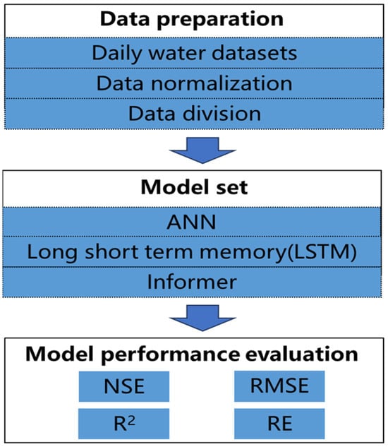
Figure 1.
The flow chart of the proposed approach for forecasting.
2.2. Deep Learning Models
2.2.1. ANN
Artificial Neural Network (ANN) is a powerful tool for dealing with machine learning problems in the computer field. It is widely used in regression and classification problems. It simulates the operation principle of biological nerve cells and forms a network structure of artificial neurons with hierarchical relationship and connection relationship. By means of mathematical expression, the signal transmission between neurons can be simulated, so as to establish a nonlinear equation with input and output relationship, and can be visualized through the network; we call it artificial neural network. Generally speaking, ANN can fit any nonlinear function through reasonable network structure configuration, so it can also be used to deal with nonlinear systems or black box models with complex internal expression.
2.2.2. Long Short-Term Memory
The LSTM network is a modified recurrent neural network proposed by Hochreiter and Schmidhuber. In recent years, the research on sequence prediction problem mainly focuses on the prediction of short sequences. LSTM network is used to conduct experiments on a set of data for short time series (12 data points, 0.5 days of data) and long time series (480 data points, 20 days of data). The results show that with the increase in sequence length, the prediction error increases significantly, and the prediction speed decreases sharply. And LSTM models have several serious problems: high prediction error—when dealing with long time series data, the prediction error of LSTM model is high, which makes it perform unsatisfactorily in some application scenarios; slow prediction speed—the LSTM model has a relatively slow prediction speed, which is mainly caused by its internal complex calculation process; more model parameters—the LSTM model has more parameters to train, which makes it require more computing resources and time when dealing with large-scale data; and prone to mode switching—when dealing with non-stationary time series data, the LSTM model is prone to mode switching, which will lead to instability of the model prediction results.
2.2.3. Informer
Recent studies have shown that compared with RNN-type models, Transformers show high potential in the expression of long-distance dependencies. However, Transformers have the following three problems: the quadratic computational complexity of self-attention mechanism—the time complexity and memory usage of each layer due to the dot product operation of self-attention mechanism; high memory usage problem—when stacking long sequence inputs, the stack of J encoder–decoder layers makes the total memory usage high, which limits the scalability of the model when accepting long sequence inputs; and efficiency in predicting long-term outputs—the dynamic decoding process of the Transformer, where the output comes one after another, and the subsequent output depends on the prediction of the previous time step, results in very slow inference.
The authors of Informer target Transformer models with the following goal: can Transformer models be improved to be more computationally, memory, and architecturally efficient while maintaining higher predictive power? To achieve these goals, this paper designs an improved Transformer-based LSTF model, namely Informer model, which has three notable features: a ProbSpare self-attention mechanism, which can achieve a low degree of time complexity and memory usage; in the self-attention distillation mechanism, a Conv1D is set on the results of each attention layer, and a Maxpooling layer is added to halve the output of each layer to highlight the dominant attention, and effectively deal with too long input sequences; and the parallel generative decoder mechanism outputs all prediction results for a long time sequence instead of predicting in a stepwise manner, which greatly improves the inference speed of long sequence prediction in Figure 2.
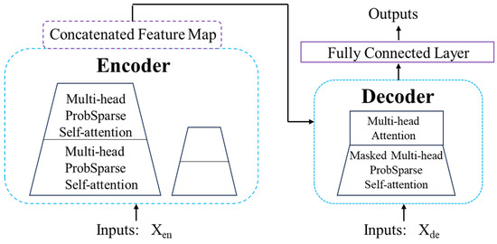
Figure 2.
Conceptual diagram of Informer.
The model belongs to the Encoder–Decoder structure, in which the self-attention distillation mechanism is located in the Encoder layer. This operation essentially consists of several encoders and aims to extract stable long-term features. The network depth of each Encoder gradually decreases, and the length of the input data also decreases, and finally, the features extracted by all encoders are concatenated. It should be noted that in order to distinguish encoders from each other, the authors gradually decrease the depth of each branch by determining the number of repetitions of the self-attention mechanism of each branch. At the same time, in order to ensure the size of the data to be merged, each branch only takes the second half of the input value of the previous branch as input.
The self-attention distillation mechanism is an efficient method to improve the efficiency and accuracy of the model by training a smaller model to guide the learning of a larger model. The core idea of the self-attention distillation mechanism is to use the attention distribution of the large model to guide the training of the small model when training the small model, so that the small model can better imitate the large model.
The principle of the self-attention distillation mechanism is that it captures the global characteristics of the input data by computing the attention distribution of the input data. Then, these features are passed to the small model so that the small model can better imitate the large model.
The generative Decoder is located in the Decoder layer. In the past time series prediction, it was often necessary to perform multi-step prediction separately to obtain the prediction results of several future time points. However, with the continuous increase of the prediction length, the cumulative error will become larger and larger, resulting in the lack of practical significance of long-term prediction. In this paper, the authors propose a generative decoder to obtain the sequence output, which only requires a single derivation process to obtain the prediction result of the desired target length, effectively avoiding the accumulation of error diffusion during multi-step prediction.
Another innovation is the probabilistic sparse self-attention mechanism, which is proposed from the author’s thinking about the feature map of the self-attention mechanism. The authors visualize Head1 and Head7 of the first layer of self-attention mechanism and find that there are only a few bright stripes in the feature map. At the same time, a small part of the scores of the two heads have large values, which is consistent with the distribution characteristics of long-tailed data, as shown in the figure above. The conclusion is that a small fraction of the dot product pairs contributes the main attention, while the others can be ignored. According to this characteristic, the authors focus on the high-scoring dot product pairs, trying to calculate only the high-scoring parts in each operation of the self-attention module, so as to effectively reduce the time and space cost of the model. It allows the model to automatically capture the relationship between the individual elements of the input sequence, so as to better understand the input sequence. This mechanism enables the model to process all elements of the input sequence in parallel, avoiding the problem of computational order dependence in sequence models such as RNN/LSTM, and thus processing more efficiently.
2.3. Model Application
The water flow data of Wan’an Reservoir is used as the dataset for prediction. The dam site of Wan’an Reservoir is located 2 km upstream of Furong Town, Wan’an County, Jiangxi Province. The upstream is 90 km away from Ganzhou City and the downstream is 90 km away from Ji’an City, and the control basin area is 36,900 square kilometers, as seen in Figure 3.
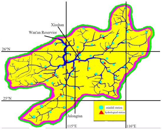
Figure 3.
Map of the Wan’an Reservoir basin.
There are several hydrological stations and rainfall stations in the basin of Wan’an Reservoir. In this paper, the rainfall information of five regions around the reservoir (PQJ1, PQJ2, PQJ3, PQJ4, and PQJ5) and the flow information of Xiashan hydrological Station and Julongtan hydrological station are selected to predict the flow of Wan’an Reservoir. In total, 1176 precipitation and discharge data were collected from a total of 28 floods in the region from 17 May 2014, to 14 June 2020, and the collection interval was 6 h. Some of the collected datasets are shown in Table 1.

Table 1.
Dataset of Wan’an reservoir.
Due to the noise and jitter of the initial data, the smooth function is used to smooth the data, and the value at time t after processing is the average value at time t − 1, t, and t + 1. In addition, the flow at the flood peak needs to be recorded, so the flow at the flood peak is not smoothed.
In this experiment, considering the long sampling time, the seq length is set to 4, 5, and 6, and the output length is 1, respectively. When the seq length is 4, four pieces of data are used to predict one piece of data in the future.
The normalization method uses max–min normalization.
The commonly used loss functions in machine learning regression problems include mean absolute error (MAE), mean square error (MSE), and Huber Loss. MSE loss usually converges faster than MAE, but MAE loss is more robust to outliers, that is, less susceptible to outliers. Huber Loss is a Loss function that combines MSE and MAE and takes the advantages of both, also known as Smooth Mean Absolute Error Loss. The principle is simple: MSE is used when the error is close to 0 and MAE is used when the error is large.
In this paper, more attention is paid to the peak flood flow since it has the greatest impact on reality, and MAE, MSE, and Huber Loss functions are used in this experiment to compare the prediction effect.
In the predictions of the two models, the common parameters are learning rate, training epochs, patience, and batch size which is 0.0005, 100, 10, and 10 respectively.
All numerical experiments in this study were implemented on a Windows system (CPU: Intel i7-12700H (Intel, Santa Clara, CA, USA), GPU: NVIDIA GeForce RTX 3070 (NVIDIA, Santa Clara, CA, USA) using Python (3.9) based on the Pytorch (1.8.0)).
2.4. Model Performance Measures
Four indicators are finally used to measure the prediction results, namely NSE (Nash coefficient), R2 (determination coefficient), RMSE (mean square error), and RE (mean difference).
Four hydrological concepts were used to measure the prediction results, namely, the number of fields with the peak discharge gap being less than 0.15, the number of fields with the total flood gap being less than 0.15, the number of fields with the Nash coefficient greater than 0.8, and the maximum flood peak gap. The calculation formulae [23] are as follows:
where xi and yi are observed and simulated values, respectively; x and y are average observed and simulated values, respectively; and n is the number of samples.
NSE (Nash coefficient): It is used to verify the quality of hydrological model simulation results. The value of NSE is negative infinity to 1, and NSE is close to 1, indicating that the model quality is good.
R2 (Coefficient of Determination): The proportion that reflects the total variation of the dependent variable can be explained by the independent variable through the regression relationship. It ranges from 0 to 1. The greater the coefficient of determination, the better the prediction effect.
RMSE (mean square error): The square root of the ratio between the squared deviation of the predicted value from the true value and the number of observations. It tells you how discrete a dataset is.
RE (mean difference): the ratio of the absolute error caused by a measurement to the measured (agreed) true value multiplied by 100%, which reflects the confidence of the measurement.
Peak discharge: The maximum instantaneous discharge in a flood discharge process, that is, the highest discharge on the flood process line. It may be the measured value, or it may be the calculated value using the water–flow relationship curve or the calculation value of the hydrodynamic formula.
Total flood water: The total amount of flood water flowing from the outlet section of the basin in a certain period of time. The total amount of a flood caused by rainfall is often calculated in the forecast of rainfall runoff, which can be obtained from the area between the beginning time of the flood flow and the end time on the retreating section of the flood process line.
3. Result
Using thirty percent of the data as the prediction set, the different seq lengths and prediction accuracy metrics based on the loss types (MAE, MSE, and Huber) of the three deep learning models (ANN, LSTM, and Informer) are shown in Table 2.

Table 2.
Wan’an reservoir forecast results table (prediction set).
In addition, considering that this study is application-oriented, the trained model is used to predict all datasets, and the results are obtained and compared with the original data, as shown in Table 3. The best results of the three models are marked in red.

Table 3.
Wan’an reservoir forecast results table (all data).
The numbers of the following four indicators are shown in Table 4: flood peak difference values less than 15%, total flood difference less than 15%, NSE more than 0.8, a max flood peak gap. Bigger is better for the first three metrics, and smaller is better for the last one. The best results of the three models are marked in red.

Table 4.
Four indicators of Wan’an reservoir prediction results table (all data).
4. Discussion
In Table 2 and Table 3, the best prediction results of the three models are marked in red, and the best prediction results are based on the statistical results of the Informer. The result with the highest NSE (Nash coefficient) is selected, that is, the seq length is four and the loss function is MAE. Two floods (No. 1 and No. 2) are selected to draw the rainfall flow diagram, see Figure 4 and Figure 5.
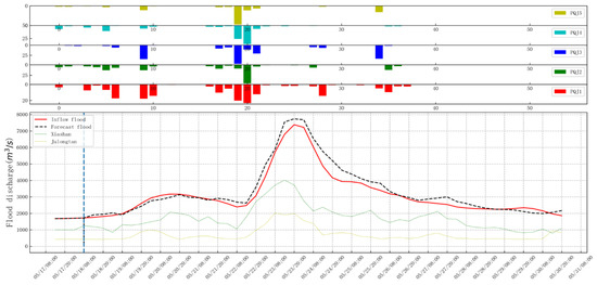
Figure 4.
No. 1 Flood rainfall flow chart (Informer).
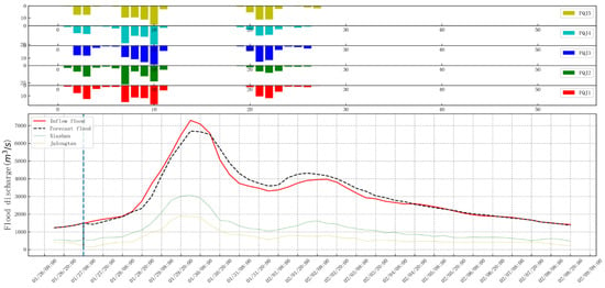
Figure 5.
No. 2 Flood rainfall flow chart (Informer).
From Figure 4 and Figure 5, it can be found that the predicted flood process line has a high degree of agreement with the actual flood process, and compared with the flood peak of Xiashan and Julongtan, the flood peak is lagged behind, which better reflects the spatiotemporal information of the flood.
According to Table 2, 30% of the data are taken as the prediction set. For four statistical indicators (NSE, R2, RMSE, and RE), the average value of three different seq length predictions is taken as the result to draw the bar chart, as shown in Figure 6, the horizontal axis is the three loss functions, and the vertical axis is the average value of the indicators. (a), (b), (c), and (d) are bar charts of the four indicators, respectively. Larger values of NSE and R2 lead to better results, while smaller values of RMSE and RE lead to better results. We can find from Figure 6 that the Informer has better NSE, RMSE, and RE, and similar R2 compared with ANN and LSTM.
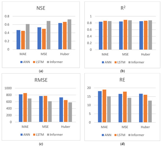
Figure 6.
Prediction results indicator bar chart (prediction set). (a) NSE bar chart, (b) R2 bar chart, (c) RMSE bar chart, (d) RE bar chart.
According to Table 3, all datasets are used for prediction, and the bar charts of the four indicators are shown in Figure 7. a–d are bar charts of the four indicators, respectively. We can find from Figure 7 that the Informer has better NSE, RMSE, RE, and R2 compared with ANN and LSTM.
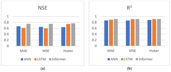
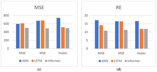
Figure 7.
Prediction results indicator bar chart. (a) NSE bar chart, (b) R2 bar chart, (c) RMSE bar chart, (d) RE bar chart.
According to Table 4, a table is made for each hydrological indicator. The average of the three different sequence length predictions is taken as the result to draw a bar graph, as shown in Figure 8. The horizontal axis shows the three different loss functions, and the vertical axis shows the number of flood fields or the maximum flood peak difference satisfying the hydrological index in the 28 floods. (a), (b), (c), and (d) are bar charts of the four indicators, respectively. Among them, a larger number of flood fields satisfying the conditions indicates a better result, and a smaller maximum flood peak difference indicates a better result. We can find from Figure 8 that the four indicators (a flood peak difference values less than 15%, a total flood difference less than 15%, NSE more than 0.8, a max flood peak gap) of the Informer are better than ANN and LSTM.
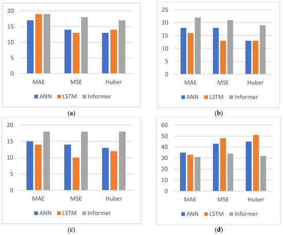
Figure 8.
Histogram of hydrographic indicators bar chart. (a) flood peak difference values less than 15%, (b) total flood difference less than 15%, (c) NSE more than 0.8, (d) max flood peak gap.
5. Conclusions
In this study, the Informer model and traditional hydrology methods were combined to study the effect of the ANN, LSTM, and Informer models in predicting the flood discharge of the Wan’an Reservoir, and NSE, RMSE, R2, and RE were used to evaluate the accuracy and reliability of the prediction, all of which showed satisfactory results. Therefore, using a machine learning method to predict flood flow is reliable. The results show that the Informer is superior to ANN and LSTM in most cases.
The R2 of the LSTM model is better than the Informer model, except for in three cases (loss = MAE, seq length = 4), (loss = MAE, seq length = 5), and (loss = MSE, seq length = 4). In other cases, the statistical indicators of the Informer model are better than the other two models. However, when predicting with the full dataset, the R2 of the LSTM model (los = MAE, seq length = 5) is better than that of the Informer model in both cases (loss = MSE, seq length = 6). In one case (loss = Huber, seq length = 5), the LSTM model has better RE than the Informer model, and in the remaining cases, the Informer model predicts the best result. In terms of hydrological indicators, LSTM outperforms the Informer in three cases, ANN outperforms the Informer in four cases, and the Informer predicts better in the remaining cases. Therefore, we can conclude that the Informer performs better than the ANN and LSTM models in predicting the Wan’an reservoir.
According to Figure 6, Figure 7 and Figure 8, we can get the final conclusion that the average values of the four indicators (NSE, R2, RMSE, and RE) of the Informer model are better than those of ANN and LSTM under nine different conditions.
However, we find that the Informer model still has the following two problems: although the prediction accuracy is higher than ANN and LSTM, there is still the possibility of improvement; the three indicators, NSE, MSE, and RE, of the Informer are better than the other two models, but the R2 of the three models are similar. Recently, the diffusion model has become popular, which works by iteratively adding noise to an image and then training a neural network to learn the noise and recover the image. It is widely used in the fields of time series data prediction and images like CSDI and GLIDE. My next research direction is to combine the diffusion model and the Informer, and use the powerful generation ability of the diffusion model and the powerful computing power of the Informer to improve the prediction accuracy and get better results.
Author Contributions
Conceptualization: J.Z. and B.W.; Investigation: Y.X.; Resources: J.W. and J.C.; Software: Y.X.; Writing—original draft: Y.X.; Writing—review & editing: J.Z. and B.W.; Supervision: J.Z. All authors have read and agreed to the published version of the manuscript.
Funding
This work was supported by the “Science and Technology + Water Conservancy” Joint Plan Project “Research and Application Demonstration of Reservoir Flood Forecasting and Dispatching Technology Based on Artificial Intelligence Driven by Big Data” (2023KSG01007), Science and Technology Department of Jiangxi Province, PRC.
Data Availability Statement
Due to the nature of this research, participants of this study did not agree for their data to be shared publicly, so supporting data is not available.
Conflicts of Interest
Author Jun Wan was employed by the company Wuhan Luoshui Intelligent Technology Co., Ltd. The remaining authors declare that the research was conducted in the absence of any commercial or financial relationships that could be construed as a potential conflict of interest.
References
- Martina, M.L.V.; Todini, E.; Libralon, A. A Bayesian decision approach to rainfall thresholds based flood warning. Hydrol. Earth Syst. Sci. Discuss. 2006, 2, 413–426. [Google Scholar] [CrossRef]
- Bartholmes, J.C.; Thielen, J.; Ramos, M.H.; Gentilini, S. The european flood alert system EFAS-Part 2: Statistical skill assessment of probabilistic and deterministic operational forecasts. Hydrol. Earth Syst. Sci. 2009, 13, 141–153. [Google Scholar] [CrossRef]
- Park, D.; Markus, M. Analysis of a changing hydrologic flood regime using the variable infiltration capacity model. J. Hydrol. 2014, 515, 267–280. [Google Scholar] [CrossRef]
- Qiao, G.C.; Yang, M.X.; Liu, Q. Monthly runoff forecast model of Danjiangkou Reservoir in autumn flood season based on PSO-SVRANN. Water Conserv. Hydropower Technol. 2021, 52, 69–78. [Google Scholar]
- Tan, Q.F.; Wang, X.; Wang, H.; Lei, X. Application comparison of ANN, ANFIS and AR models in daily runoff time series prediction. S. N. Water Transf. Water Conserv. Sci. Technol. 2016, 14, 12–17+26. [Google Scholar]
- Salas, J.D.; Markus, M.; Tokar, A.S. Streamflow forecasting based on artificial neural networks. Artif. Neural Netw. Hydrol. 2000, 36, 23–51. [Google Scholar]
- Tokar, A.S.; Johnson, P.A. Rainfall-runoff modeling using artificial neural networks. J. Hydrol. Eng. 1999, 4, 232–239. [Google Scholar] [CrossRef]
- Liu, H. Research on flood classification and prediction based on neural network and genetic algorithm. Water Resour. Hydro Power Technol. 2020, 51, 31–38. [Google Scholar]
- Li, D.Y.; Yao, Y.; Liang, Z.M.; Zhou, Y.; Li, B. Hydrological probability prediction method based on variable decibel Bayesian depth learning. Water Sci. Prog. 2023, 34, 9. [Google Scholar]
- Xu, Y.; Hu, C.; Wu, Q.; Jian, S.; Li, Z.; Chen, Y.; Zhang, G.; Zhang, Z.; Wang, S. Research on particle swarm optimization in LSTM neural networks for rainfall-runoff simulation. J. Hydrol. 2022, 608, 553. [Google Scholar] [CrossRef]
- Cui, Z.; Guo, S.L.; Wang, J.; Wang, H.; Yin, J.; Ba, H. Flood forecasting research based on GR4J-LSTM hybrid model. People Yangtze River 2022, 53, 1–7. [Google Scholar]
- Ouyang, W.Y.; Ye, L.; Gu, X.Z.; Li, X.Y.; Zhang, C. Review of the progress of in-depth study on hydrological forecasting II—Research progress and prospects. S. N. Water Transf. Water Conserv. Technol. 2022, 20, 862–875. [Google Scholar]
- Yin, H.; Wang, F.; Zhang, X.; Zhang, Y.; Chen, J.; Xia, R. Rainfall-runoff modeling using long short-term memory based step-sequence framework. J. Hydrol. 2022, 610, 901. [Google Scholar] [CrossRef]
- Li, B.; Tian, F.Q.; Li, Y.K.; Ni, G. Deep-learning hydrological model integrating temporal and spatial characteristics of meteorological elements. Prog. Water Sci. 2022, 33, 904–913. [Google Scholar]
- Vaswani, A.; Shazeer, N.; Parmar, N.; Uszkoreit, J.; Jones, L.; Gomez, A.N.; Kaiser, L.; Polosukhin, I. Attention is all you need. Neural Inf. Process. Syst. 2017, 5998, 008. [Google Scholar]
- Schwaller, P.; Laino, T.; Gaudin, T.; Bolgar, P.; Hunter, C.A.; Bekas, C.; Lee, A.A. Molecular transformer: A model for uncertainty-calibrated chemical reaction prediction. ACS Cent. Sci. 2019, 5, 1572–1583. [Google Scholar] [CrossRef]
- Wang, W.; Xie, E.; Li, X.; Fan, D.-P.; Song, K.; Liang, D.; Lu, T.; Luo, P.; Shao, L. Pyramid vision transformer: A versatile backbone for dense prediction without convolutions. In Proceedings of the 2021 IEEE/CVF International Conference on Computer Vision (ICCV), Montreal, QC, Canada, 10–17 October 2021; pp. 548–558. [Google Scholar]
- Zhou, C.H.; Lin, P.Q. Traffic volume prediction method based on multi-channel transformer. Comput. Appl. Res. 2023, 40, 435–439. [Google Scholar]
- Dong, J.F.; Wan, X.; Wang, Y.; Ye, R.; Xiong, Z.; Fan, H.; Xue, Y. Short-term power load forecasting based on XGB-Transformer model. Power Inf. Commun. Technol. 2023, 21, 9–18. [Google Scholar]
- Li, S.; Jin, X.; Xuan, Y.; Zhou, X.; Chen, W.; Wang, Y.X.; Yan, X. Enhancing the locality and breaking the memory bottleneck of transformer on time series forecasting. Neural Inf. Process. Syst. 2019, 32. preprint. [Google Scholar]
- Liu, C.; Liu, D.; Mu, L. Improved transformer model for enhanced monthly streamflow predictions of the Yangtze River. IEEE Access 2022, 10, 58240–58253. [Google Scholar] [CrossRef]
- Zhou, H.Y.; Zhang, S.H.; Peng, J.Q.; Zhang, S.; Li, J.; Xiong, H.; Zhang, W. Informer: Beyond efficient transformer for long sequence time series forecasting. In Proceedings of the 35th AAAI Conference on Artificial Intelligence, the 33rd Conference on Innovative Applications of Artificial Intelligence, the 11th Symposium on Educational Advances in Artificial Intelligence, Virtual Event, 2–9 February 2021; AAAI: Menlo Park, CA, USA, 2021; pp. 11106–11115. [Google Scholar]
- Li, G.; Liu, Z.J.; Zhang, J.W.; Han, H.; Shu, Z.K. Bayesian model averaging by combining deep learning models to improve lake water level prediction. Sci. Total Environ. 2024, 906, 167718, ISSN 0048-9697. [Google Scholar] [CrossRef] [PubMed]
Disclaimer/Publisher’s Note: The statements, opinions and data contained in all publications are solely those of the individual author(s) and contributor(s) and not of MDPI and/or the editor(s). MDPI and/or the editor(s) disclaim responsibility for any injury to people or property resulting from any ideas, methods, instructions or products referred to in the content. |
© 2024 by the authors. Licensee MDPI, Basel, Switzerland. This article is an open access article distributed under the terms and conditions of the Creative Commons Attribution (CC BY) license (https://creativecommons.org/licenses/by/4.0/).