Estimating Climate Change’s Impacts on the Recharge of an Ungauged Tropical Aquifer (Togolese Coastal Sedimentary Basin)

Abstract

The aquifers of the Togolese coastal sedimentary basin are the principal sources of water for almost half of the country’s population. These aquifers’ features have not been adequately monitored and studied. The resource is threatened by human activities, notably agriculture, industry, and withdrawals for drinking water supplies. This situation is exacerbated by the potential effects of climate change. For this research, a basin-scale study was conducted to estimate current groundwater recharge and its future evolution in response to climate change. A recharge model based on Thornthwaite–Mather balance equations using runoff coefficients characterizing land use was fed with current and future climate data from an optimistic scenario (RCP 4.5) and a pessimistic scenario (RCP 8.4). Despite the associated uncertainties, the soil–water balance model at monthly time steps predicts a recharge of 3 to 455 mm per year from 2020 to 2039, and 40 to 420 mm per year from 2040 to 2059 under the optimistic RCP 4.5 scenario. According to the pessimistic RCP 8.5 scenario, the recharge will range between 16 and 515 mm per year from 2020 to 2049 and from 1 to 467 mm per year between 2040 and 2059. As a result, the basin’s groundwater recharge range, which is currently 47 to 225 mm, will significantly increase. This study provides a scientific basis for the sustainable management of groundwater in the Togolese coastal sedimentary basin. The recharge of the groundwater in the basin will increase regardless of the climate scenario and will support future development in the Togolese coastal sedimentary basin.

1. Introduction

Climate change is real [1], and it will modify the water cycle [2,3]. The hydrological cycle is affected by climatic variations and the interactions between precipitation, temperature, and evapotranspiration [4,5,6,7,8,9,10,11]. As a result, each change in the climate system induces a difference in the water system and vice versa [4], resulting in variations in water availability over time and space. Water excesses or deficits are likely to increase the severity of extreme weather events [12,13], including floods and droughts. The risk of deficit is, for its part, accentuated due to the overexploitation of water resources already observed in many regions of the world [14,15,16,17]. The impacts of climate change also manifest themselves on a social [18,19] and economic level, with the weakening of production systems [20,21,22], particularly in agriculture [23]. They are also illustrated by the increase in drilling costs, the reduction in well yields [24], and threats to ecosystems [25,26]. Finally, also due to climate change, pollution and the degradation of the quality of water resources from anthropogenic activities are accentuated [4,27,28,29].

This is why climate change is on the political agenda at the national and international levels [1], and also because regional adaptation strategies rely on water resources [30,31,32,33,34]. Assessments of the impacts of climate change on water resources have, therefore, become essential, with those concerning groundwater being even more essential because they represent approximately 98% of global freshwater resources [4,35].

Studies on the impacts of climate change on groundwater have multiplied in recent years, and they often focus on the evolution of recharge [4]. This is because precipitation and temperature determine the availability and movement of water in the environment, which, in turn, influences groundwater recharge rates [31]. It is then useful for authorities to know about the trends in groundwater recharge over time and space so they can make appropriate arrangements and develop effective water resources management plans [31,36,37,38].

Recharge is defined herein as the downward flow of water reaching the water table, adding to the groundwater storage [39]. However, the rate of aquifer recharge is one of the most difficult factors to measure when evaluating groundwater resources [36] and, by whatever method, is normally subject to many uncertainties and errors [40]. In fact, groundwater recharge depends on several factors, such as hydraulic conditions and the scale of estimation [38]. It should also be noted that unmanaged contexts may differ significantly from managed conditions, as recharge may vary depending on system boundary conditions. In addition, the determination of recharge variability in space and time, which is high, creates a number of unresolved problems that require additional investigation [36].

Groundwater recharge is generally estimated based on monitoring well data and measurements. The most common methods for estimating groundwater recharge are the soil–water balance method, the zero flux plane method, the one-dimensional soil–water flow model, the inverse modeling technique, the groundwater level fluctuation method, the hybrid water fluctuation method, the groundwater balance method, and isotope and solute profile techniques [40,41]. However, in many areas of the world [42], especially in sub-Saharan Africa, spatial and temporal coverage is scarce, and in situ measurements are nonexistent because they are relatively expensive [43]. Expense is a common limitation when applying some recharge estimation methods [44]. When considering such challenges, the water-budget method proves to be the most suitable because it is universal and adaptable [39]. Water budgets are fundamental to the conceptualization of hydrologic systems at all scales [39]. Building a preliminary water budget from existing data is an easy and logical first step in any study, regardless of whether water-budget methods will subsequently be used to estimate recharge [39]. It is based on the principle that the water input is equal to the quantity released plus (or minus) the change in the volume of water stored [45]. The balance can be estimated with semiempirical equations using precipitation and temperature, indirect estimates of evapotranspiration, and runoff [39,45,46,47]. Using these approaches, it is possible to estimate the recharge rate of a specific aquifer over extended areas, such as at the watershed scale [45]. Despite the uncertainties inherent in this method, it provides relevant information in terms of the characterization of anthropogenic and climate impacts on groundwater at a low cost and with few resources [11,30,48,49,50,51,52,53].

On a global scale, the worst projections related to reductions in recharge were identified for arid and desert areas; the highest recharges were identified in the northern regions and in areas at high altitudes, where recharge capacity is maintained or increases due to rapid snow and glacial melting from temperature increases [4]. Despite the advances achieved, more studies should be undertaken to analyze groundwater assessment at other latitudes to reach a complete and comprehensive understanding [4].

In Africa, characterizing the impacts of climate change on groundwater is crucial, due to the fact that more than half of the population depends on groundwater for their needs and economic activities [54]. In a continent where human and material resources are often limited, groundwater has the advantage of generally being of good quality and abundant [55]. This interest is also explained by the fact that groundwater has a buffering effect that mitigates the seasonal water availability fluctuations [56], which is a notable advantage in the face of climate change. However, there are questions, especially about the long-term renewability of groundwater in the African context. These questions are part of a more general reflection on the potential impacts of climate change on groundwater in Africa, in the face of increasing withdrawals, growing pollution, poor monitoring of the resource, and the uncertainties inherent in climate change and modeling [57].

On the African continent, work must be carried out on a case-by-case basis, due to complex local dynamics. If, in the Sahel and southern Africa, the trend is toward a future decline in recharge [33,58,59,60,61], other areas will experience notable increases in recharge, particularly in tropical and equatorial climates [32], due to climate change.

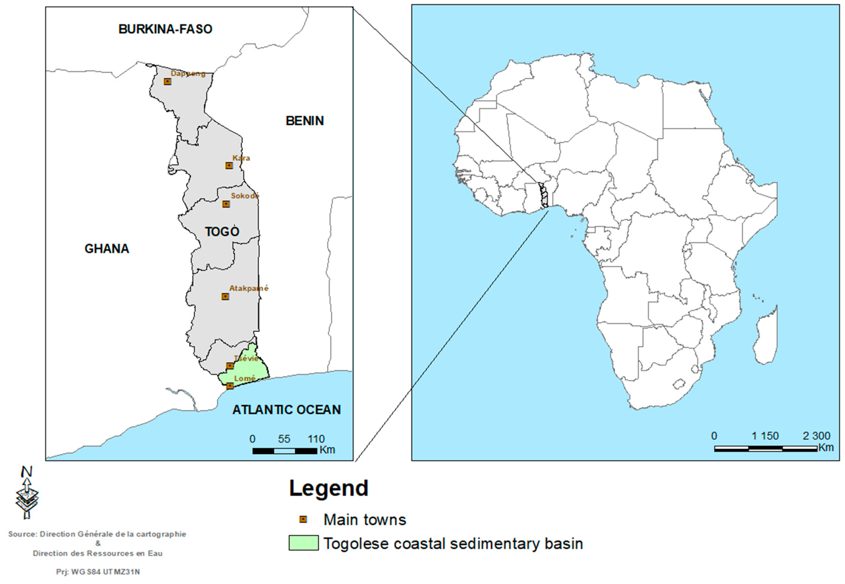
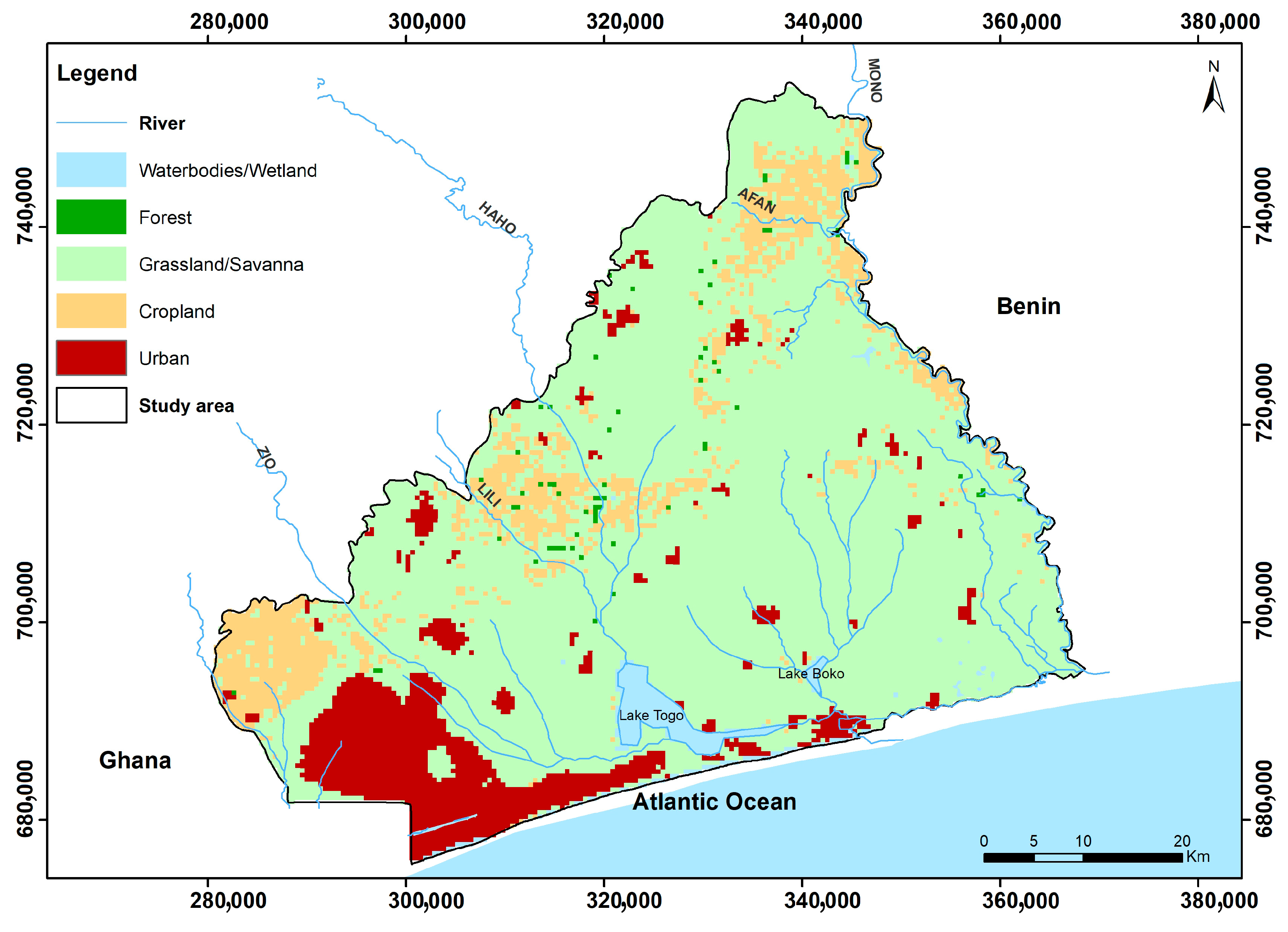
This study aims to estimate the current and future groundwater recharge in an aquifer system located in the Togolese coastal sedimentary basin in West Africa. This less-monitored aquifer is in an area marked by strong economic and demographic growth. This translates into significant water withdrawals associated with pollution risks, all within the context of climate change. Because of the region’s economic importance, the basin is undergoing rapid urbanization. This has resulted in increased groundwater abstraction, as well as pollution problems caused by inadequate sanitation infrastructure. It is important for decision makers to know how recharge will evolve over time and space, and therefore the future availability of groundwater. This will enable them to make the best choices in terms of decision making.

For this purpose, this study used the simple and robust Thornthwaite and Mather method [47]. The originality of this study, considering the rarity of the available data, lies in the use of data freely available on the Web (such as current and future local climate data, elevation models, and land-use data). All data were used to identify water balance parameters to support groundwater resource management strategies.

2. Materials and Methods

2.1. Study Area

The coastal sedimentary basin of Togo covers 3500 km² and is in the maritime region situated in the extreme south of Togo, bordering the Atlantic Ocean (Figure 1). In all, 50% of the population is concentrated in less than 10% of its territory, making it the political and economic heart of the country. Groundwater contributes, almost completely, to satisfying human water demand and economic activities [62]. The morphology shows plateaus sloping toward the south with an elevation below 150 m. The basin has a humid tropical climate [63] characterized by a long rainy season from April to June and a brief rainy season from September to October, separated by dry seasons. From 1991 to 2020, the average annual precipitation ranged from 800 mm near the coast to 1400 mm north of the basin, and the average annual air temperature ranges from 24 to 30 °C. Land cover is characterized by settlements with a high proportion of bare soil surrounded by savannah, cropland, and water bodies [64,65].

The geology of the basin comprises two sedimentary series covering the crystalline basement (Figure 2 and Figure 3): Maastrichtian/Eocene deposits (sand, marly limestone, marl, and clay) and a Quaternary series of continental and coastal origin resting horizontally and unconformably on the marine series [66]. The groundwater consists mainly of water flowing in the unconfined sand-and-gravel aquifer of the Continental Terminal, the confined aquifer in the Paleocene sand and limestone, and the semi-confined aquifer in the Maastrichtian sand [67,68,69,70]. Groundwater monitoring started in 2015 with some piezometers, with an irregularity in the frequency of measurements that does not yet allow for a relevant analysis.

The soils of the area are predominantly sandy and clayey with some silty layers [71]. Five types of soil dominate the basin [71,72]: soils that have evolved little, such as erosion soils, contribution soils, and verticals; hydromorphic and tropical ferruginous soil concretions; non-indurated ferralitic soils; flooded, advanced, and hydromorphic soils in alluvial valleys; and marine sands of the coastline and lagoons. Over 60% of the soils in the maritime region where the basin is located are moderately or significantly degraded, while only 35% are slightly degraded. Soils that have not deteriorated are almost nonexistent. Urbanization, mining (phosphate, limestone, gravel, etc.), quarrying (sand, gravel, etc.), and coastal erosion are the main causes of this degradation trend.

To characterize groundwater recharge under current conditions, we relied on climatic conditions over the past 30 years (1991–2020). The current climate data are produced by the Climatic Research Unit (CRU) of the University of East Anglia, and data are presented at a 0.5° × 0.5° (50 km × 50 km) resolution [73,74]. The current tropical climate has average temperatures that oscillate between 26 and 28 °C during the year. Rainfall has two peaks that characterize the long rainy season from March to July and the short rainy season from September to November (Figure 4).

2.2. Methodology

The Thornthwaite–Mather water balance approach was selected for the recharge estimation [75]. This method of monthly accounting is predicated on the idea that the amount of water in the soil (including the partially saturated zone) can be conceptualized by a single water stock value (Si) stated in millimeters at the end of month i with a maximum water stock capacity (Smax). Depending on whether Pi (rainfall in month i) is more or less than PETi (potential evapotranspiration in month i), moisture is either added to or withdrawn from the total. The estimation of excess water is based on both runoff and groundwater recharge, and if Si rises, it cannot exceed Smax. When Si falls, its value cannot be less than zero, resulting in a probable water deficit and ETi (evapotranspiration for month i) being less than PETi.

In the first stage, a surface runoff map is built to calculate the infiltrated rain by overlaying maps of soil, land cover, and terrain slope according to their permeability capacities (Figure 5). It is derived from the many maps that have been assigned coefficients. The soil permeability map is created by reclassifying the region’s soil map based on its qualities and the percentage of clay/silt or organic matter. Sandy (high permeability or low runoff), silty (middle permeability or medium runoff), and clayey (low permeability or heavy runoff) are the three categories. Land use is used to generate the infiltration capacity map. As a result, the soil types are classed based on their infiltration capacity. Finally, the slope map is generated using the reclassified digital elevation model (DEM) of the study area. The soil permeability, land cover infiltration capacity, and terrain slope maps were input into an QGIS database and processed to produce the final surface runoff map (Figure 5).

The objective of the second step is to estimate the amount of water that can reach the aquifer based on climatic conditions (temperatures and precipitation) for each class of runoff coefficient. At each time step, soil moisture is calculated from the balance between what enters the soil by precipitation and what leaves it by evapotranspiration until the field capacity of a soil is reached.

In the third and final stage, the recharge values obtained are grouped together to produce a map of the groundwater recharge zone. In detail, the water balance equation is used to calculate the change in soil moisture (∆S) over successive months through the following equation:

∆S = S_i − S_i−1

(1)

where S_i and S_i−1 are soil moisture storage values in the current month and the previous month, respectively.

According to the change in soil moisture storage of the current month, current evapotranspiration (AE) is calculated using the following:

AE = PET, when P ≥ PET
AE = P + ∆S when P < PET

(2)

where P is the precipitation and PET is the potential evaporation; the soil moisture deficit (D) is taken as the difference between PE and AE (Equation (2)), while the surplus is calculated using P, PE, and S as follows:

D = PET – AE

(3)

When the conditions allow, the recharge is obtained (when P > PET) in the following way:

R = S_i−1 + (P − PET)_i − Smax; when S_i = S_max

(4)

2.2.1. Data Collection

Our study is based on current and future monthly temperature and precipitation data for the maritime region covering the study area, which are available on the World Bank’s Climate Change Knowledge Portal [76]. Monthly potential evapotranspiration was estimated using the empirical formula created by Thornthwaite (1948), which requires only air temperature data [39].

The current and future monthly potential evapotranspiration were calculated from the monthly heat index for the 5° N latitude where the basin is located and the current and future monthly temperatures.

In addition to temperatures and precipitation, the water balance data collected for the study include soil moisture and the runoff coefficient. These are terms from within the water balance that are not directly available and are based on the literature, the soil map of Togo [71], the Shuttle Radar Topography Mission (SRTM) topographic data [77], and the MODIS Land Cover image [78] of the area.

2.2.2. Groundwater Recharge Estimation

• The following sections detail the methods for estimating soil moisture (WS) and surface runoff (C) as well as the procedure for estimating recharge at the basin scale.

Soil moisture or the soil water content for a given month is calculated as follows:

WS = (WS_max) 10^b(Inf-PET).

(5)

where WS_max is the water-storing capacity of the soil, Inf is the infiltration during the month, PET is the potential evapotranspiration during the month, and b is a coefficient determined as follows [79]:

b = 0.455/(WS_max)

(6)

In our study, the WS_max value is 100 mm. In the absence of specific studies on the area, we retained this value from recent work in the neighboring regions to the north in the Mono Basin and to the east in Benin [80,81].

• Runoff classes estimation

We determined the runoff from a runoff coefficient C, according to Equation (1) proposed by the American Society of Civil Engineers (ASCE) [82] (

Table 1. Values of the coefficients for runoff calculation adapted for the study area from the ASCE [82] tabulation.

Type of Area		C′
Soil (C′1)	Clay	0.1
	Silt	0.2
	Sand	0.4
Land cover (C′2)	Cropland	0.1
	Urban	0.1
	Grassland/Savanna	0.2
	Forest	0.2
Slope (C′3)	<2%	0.3
	2–7%	0.2
	>7%	0.1

), which represents the portion of rainfall that is converted to runoff before entering the soil budget calculation [45,46].

C = 1 − (C′₁ + C′₂+ C′₃),

(7)

Here, C′₁ is the soil permeability coefficient, C′₂ is the infiltration capacity coefficient, and C′₃ is the slope coefficient.

⚬

Soil permeability coefficient (C′₁): This was obtained from the soil map of Togo [71] by reclassifying soils into three types according to grain size: low (clay), moderate (sandy loam), and high permeability (sand).

⚬

Infiltration capacity coefficient (C′₂): To characterize land cover and thus infiltration capacity, we used MODIS satellite imagery of the study area taken in 2019 [78]. The image was reclassified according to the infiltration capacities contained in Table 1.

⚬

Slope coefficient (C′₃): The slope coefficient over the basin was generated as a map (Figure 6) from the STRM data [77]. Three slope intervals were defined: <2% (low slopes) with C′₃ = 0.3; 2-7% (moderate slopes) with C′₃ = 0.2; and >7% (high slopes) with C′₃ = 0.1 [45,46,82].

Using the data described above, one may estimate groundwater recharge at any site in the basin based on its surface runoff coefficient. Appendix A describes the details of the recharge estimation technique [41,42,45,46].

2.2.3. Modeling Scenarios

In the following section, we sought to estimate the groundwater recharge in the basin under current and future climate conditions. Here, current and future climate data for the marine region where the study area is located are presented and described.

The future climate data for the region are CMIP5 [83] indicators investigated as a multi-model ensemble, presented at 1.0° × 1.0° (100 km × 100 km) resolution. Following global climate warming, the climate scenarios over the basin are RCP 2.6, RCP 4.5, RCP 6.0, and RCP 8.5, i.e., from the most optimistic to the most pessimistic [84] (Figure 6).

Figure 6. Projected mean temperature in the maritime region, Togo; (Ref, Period: 1986–2005), Multi-Model Ensemble [84].

Figure 6. Projected mean temperature in the maritime region, Togo; (Ref, Period: 1986–2005), Multi-Model Ensemble [84].

For our study, we did not retain the RCP 2.6 and RCP 6.0 scenarios. Indeed, RCP 2.6 seemed to us, at this stage, to be too optimistic and, thus, not very realistic. Then, between RCP 6.0 and RCP 4.5, we retained the latter because, until 2060, which is the horizon of our study, the two scenarios present similar trends. The estimation of future groundwater recharge was therefore based on the RCP 4.5 scenario for the optimistic option and RCP 8.4 (Figure 7 and Figure 8) for the pessimistic evolution. The RCP 4.5 scenario [85] is an intermediate pathway that places the stable warming level at around 4.5 W/m². The worst-case scenario RCP 8.5 is a reference scenario and represents the highest RCP scenario for GHG emissions without any explicit climate policy leading to 8.5 W/m² in 2100 [86].

The climate projections predict an increasing trend in temperature (up to +2° and +2.5°) and precipitation (up to +125 and +170 mm) in the region under all scenarios. However, the RCP 4.5 scenario shows smaller increases than the RCP 8.5 scenario. In other words, the pessimistic scenario will see a higher rainfall and temperature than the optimistic scenario. It is important to keep in mind that this difference will become more prominent over time. The increase will be greater between 2040 and 2059 than between 2020 and 2039 (Figure 7 and Figure 8).

Note that the distribution of annual precipitation will also change. Increases will be more pronounced during the short rainy season. Ultimately, the two peaks will merge into a single rainy season from March to November (Figure 7 and Figure 8).

3. Results

3.1. Soil Permeability Map

The soil permeability map (Figure 9) shows a basin consisting mostly of sandy loam. The sands are located on the Atlantic coastline and riverbeds, while the clays are concentrated in the near upstream part of Lake Togo.

3.2. Land Cover Map

The result obtained in the form of a map (Figure 10) distinguishes between areas of high permeability (forest and grassland/savanna with C′₂ = 0.2), which comprise most of the basin, and areas of medium and low permeability (cropland and urban with C′₂ = 0.1).

3.3. Slope Map

Figure 11 shows relatively flat topographic slopes, mainly 2%. Gradients between 2% and 7% are usually on the banks, while gradients above 7% are almost nonexistent.

3.4. Runoff Coefficient Map

Computation of the runoff coefficient: the application of Formula (7) with the different values of C₁, C₂, and C₃ identified previously allowed us to determine the values of C that can be obtained in the basin (

Table 2. Values for runoff coefficient (C) adopted.

Soil Permeability	C′1	Infiltration Capacity	C′2	Slope	C′3	Runoff Coefficient. C
High permeability	0.4	Forest	0.2	<2%	0.3	0.1
	0.4		0.2	2–7%	0.2	0.2
	0.4		0.2	>7%	0.1	0.3
	0.4	Grass/Sav	0.2	<2%	0.3	0.1
	0.4		0.2	2–7%	0.2	0.2
	0.4		0.2	>7%	0.1	0.3
	0.4	Cropland	0.1	<2%	0.3	0.2
	0.4		0.1	2–7%	0.2	0.3
	0.4		0.1	>7%	0.1	0.4
	0.4	Urban	0.1	<2%	0.3	0.2
	0.4		0.1	2–7%	0.2	0.3
	0.4		0.1	>7%	0.1	0.4
Moderate permeability	0.2	Forest	0.2	<2%	0.3	0.3
	0.2		0.2	2–7%	0.2	0.4
	0.2		0.2	>7%	0.1	0.5
	0.2	Grass/Sav	0.2	<2%	0.3	0.3
	0.2		0.2	2–7%	0.2	0.4
	0.2		0.2	>7%	0.1	0.5
	0.2	Cropland	0.1	<2%	0.3	0.4
	0.2		0.1	2–7%	0.2	0.5
	0.2		0.1	>7%	0.1	0.6
	0.2	Urban	0.1	<2%	0.3	0.4
	0.2		0.1	2–7%	0.2	0.5
	0.2		0.1	>7%	0.1	0.6
Low permeability	0.1	Forest	0.2	<2%	0.3	0.4
	0.1		0.2	2–7%	0.2	0.5
	0.1		0.2	>7%	0.1	0.6
	0.1	Grass/Sav	0.2	<2%	0.3	0.4
	0.1		0.2	2–7%	0.2	0.5
	0.1		0.2	>7%	0.1	0.6
	0.1	Cropland	0.1	<2%	0.3	0.5
	0.1		0.1	2–7%	0.2	0.6
	0.1		0.1	>7%	0.1	0.7
	0.1	Urban	0.1	<2%	0.3	0.5
	0.1		0.1	2–7%	0.2	0.6
	0.1		0.1	>7%	0.1	0.7

). C thus varied from 0.1 for low runoff areas to 0.7 for high runoff areas.

The same operation was performed on the C₁, C₂, and C₃ coefficient maps using QGIS software. The resulting runoff coefficient (C) map (Figure 12) shows C values ranging from 0.1 to 0.6. Indeed, due to the resolution (500 m), slopes higher than 7% located on the cliffs around the quarries were ignored.

This mapping work revealed that the runoff coefficients are unevenly distributed across the basin (

Table 3. Spatial distribution of runoff coefficients in the basin.

Surface Runoff Coef C	Surface
	km2	in %
C6	28.0	1%
C5	138.3	4%
C2	241.7	7%
C1	322.8	10%
C4	997.1	29%
C3	1659.2	49%

). Half the basin has a runoff coefficient of 0.3 (C3). These are areas with low slopes (<2%) covered by savannah or grassland. Areas with a runoff coefficient of 0.4 (C4) are also important in the basin. They cover almost 30% of its surface area and correspond to urban areas located in low-slope zones (<2%).

3.5. Current Groundwater Recharge Map

The introduction of current climate data into the recharge calculation model for all runoff coefficient classes provided the results contained in

Table 4. Recharge under the current climate computation.

Surface Runoff Coef C	Jan	Feb	Mar	Apr	May	Jun	Jul	Aug	Sep	Oct	Nov	Dec	Total
0.1				12.0	0.0	106.5	16.0		32.7	57.5			224.7
0.2					31.4	72.3	12.6		21.7	42.5			180.5
0.3						53.4	1.3		10.5	27.4			92.6
0.4						34.5				12.3			46.7
0.5
0.6
Maximum potential monthly recharge (mm)				12.0	31.4	266.6	30.0		64.9	139.6			544.5

. Under the current climate, it is noted that recharge is only possible on land with runoff coefficients between 0.1 and 0.4. The recharge ranges associated with these coefficients are spatially between 225 and 47 mm per year, for an average current groundwater recharge of about 136 mm.

Over the course of the year, there are two clear peaks in recharge in response to the two rainy seasons. The first recharge peak is related to the major rainy season, followed by a second, smaller peak after the minor rainy season (Figure 13). They correspond to the months in which the water table rises in the current period.

To better appreciate the distribution of recharge at the basin scale, the runoff coefficient map was reclassified with the corresponding recharge values. The current recharge map obtained (Figure 14) shows that the areas with medium (93 mm) and high (225 mm) recharge are located in the sandy soils (especially on the coast) and in the alluvial deposits on both sides of the riverbeds. Recharge is rather low (47 mm) in agricultural areas (cropland) and areas on sandy loam soils. Finally, recharge is zero in urbanized areas and areas on clay-type soils.

3.6. Future Groundwater Recharge

• RCP 4.5 scenario in 2020–2039 and in 2040–2059

The introduction of climate projections according to the RCP 4.5 scenario over the period 2020–2059 into the recharge model provided the results contained in

Table 5. Recharge under the RCP 4.5 scenario in the 2020–2039 computation.

Surface Runoff Coef C	Jan	Feb	Mar	Apr	May	Jun	Jul	Aug	Sep	Oct	Nov	Dec	Total
0.1						109.1	76.7	104.4	86.9	79.6			456.7
0.2						82.6	63.3	82.7	68.0	61.2			357.8
0.3						56.4	49.2	61.2	49.2	42.9			258.8
0.4						30.4	34.4	40.0	30.4	24.6			159.8
0.5						4.8	19.1	18.9	11.7	6.3			60.7
0.6							3.3						3.3
Maximum potential monthly recharge (mm)						283.3	246.0	307.1	246.2	214.6			1297.2

and

Table 6. Recharge under the RCP 4.5 scenario in the 2040–2059 computation.

Surface Runoff Coef C	Jan	Feb	Mar	Apr	May	Jun	Jul	Aug	Sep	Oct	Nov	Dec	Total
0.1						78.2	108.4	90.2	84.3	59.4			420.4
0.2						58.6	86.1	70.5	65.6	42.7			323.5
0.3							63.7	50.8	46.9	26.0			187.5
0.4							41.4	31.2	28.3	9.4			110.2
0.5							19.1	11.5	9.6				40.2
0.6
Maximum potential monthly recharge (mm)						136.8	318.7	254.1	234.6	137.5			1081.8

. Thus, depending on the streamflow coefficient, the annual recharge in the basin will be between 3.31 mm (for C = 0.6) and 456.71 mm (for C = 0.1). In this scenario, areas with runoff coefficients of 0.5 and 0.6 have recharges contrary to what was observed in the previous 30 years. Finally, in the period 2040–2059, during the year, the recharge process will take place in a single phase, unlike the two peaks observed in the current period This trend is explained by the general increase in precipitation that characterizes this scenario over these periods.

It is also noted that recharge thresholds will be lower in the 2040–2059 period than in the 2020-2039 period. This is because precipitation will be higher than in the current period but lower in 2040–2059 than in 2020–2039 (Figure 7b and Figure 8b).

• RCP 8.4 scenario in 2020–2039 and in 2040–2059

Table 7. Recharge under the RCP 8.4 scenario in the 2020–2039 computation.

Surface Runoff Coef C	Jan	Feb	Mar	Apr	May	Jun	Jul	Aug	Sep	Oct	Nov	Dec	Total
0.1						78.8	125.4	126.9	104.3	79.9			515.5
0.2						59.6	101.5	103.6	83.6	61.3			409.6
0.3					0.4		77.6	80.2	62.8	42.7			263.8
0.4							53.7	56.8	42.1	24.1			176.7
0.5							29.8	33.4	21.4	5.5			90.1
0.6							5.9	10.0	0.6				16.5
Maximum potential monthly recharge (mm)					0.4	138.5	394.0	410.9	314.8	213.7			1472.3

and

Table 8. Recharge under the RCP 8.4 scenario in the 2040–2059 computation.

Surface Runoff Coef C	Jan	Feb	Mar	Apr	May	Jun	Jul	Aug	Sep	Oct	Nov	Dec	Total
0.1						66.0	122.3	115.3	77.8	85.9			467.3
0.2						47.2	97.8	92.5	59.2	65.8			362.4
0.3						28.3	73.4	69.6	40.6	45.7			257.6
0.4							49.0	46.7	22.0	25.6			143.4
0.5							24.6	23.9	3.5	5.5			57.4
0.6							0.1	1.0					1.1
Maximum potential monthly recharge (mm)						141.5	367.2	349.0	203.0	228.5			1289.3

present the results from the recharge model using climate data under scenario 8.4. They show the same observations and trends as in scenario 4.5. Except that, in this case, the values are significantly higher.

For example, for C = 0.1 the recharge reaches 515 mm and for the least favorable areas (C = 0.6) the recharge is over 16 mm. As such, the 4.5 scenario, the 2040–2059 period, which is less rainy than the 2020–2039 period (Figure 7b and Figure 8b), consequently shows lower recharge.

4. Discussion

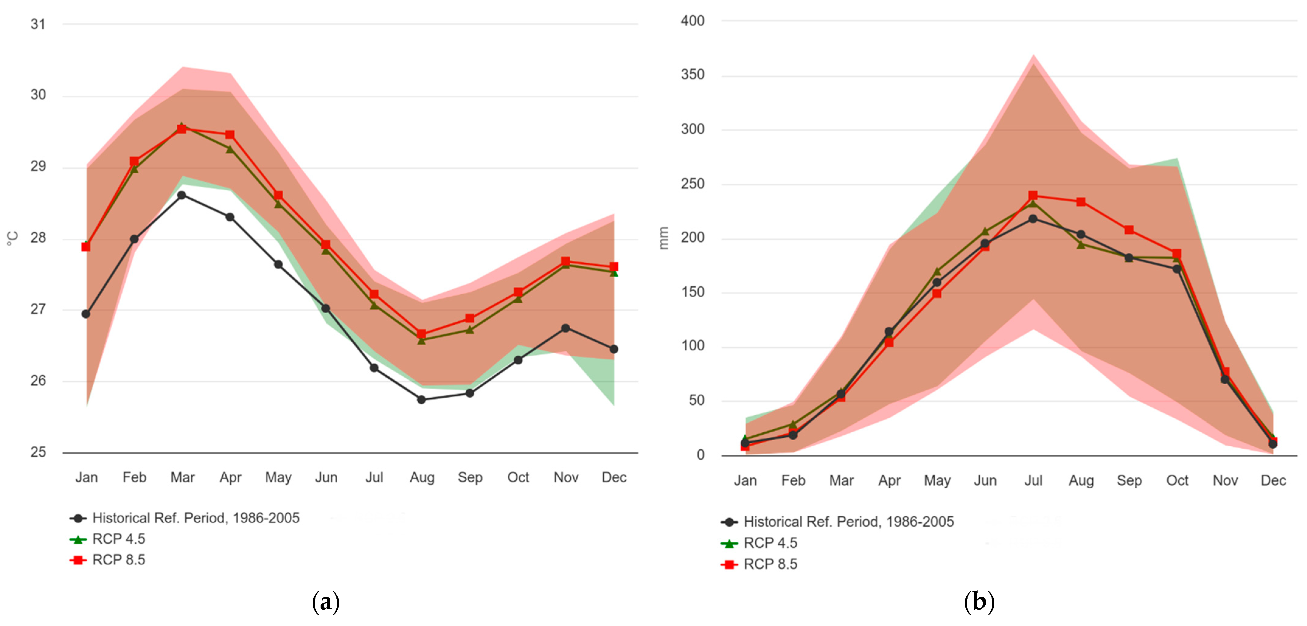
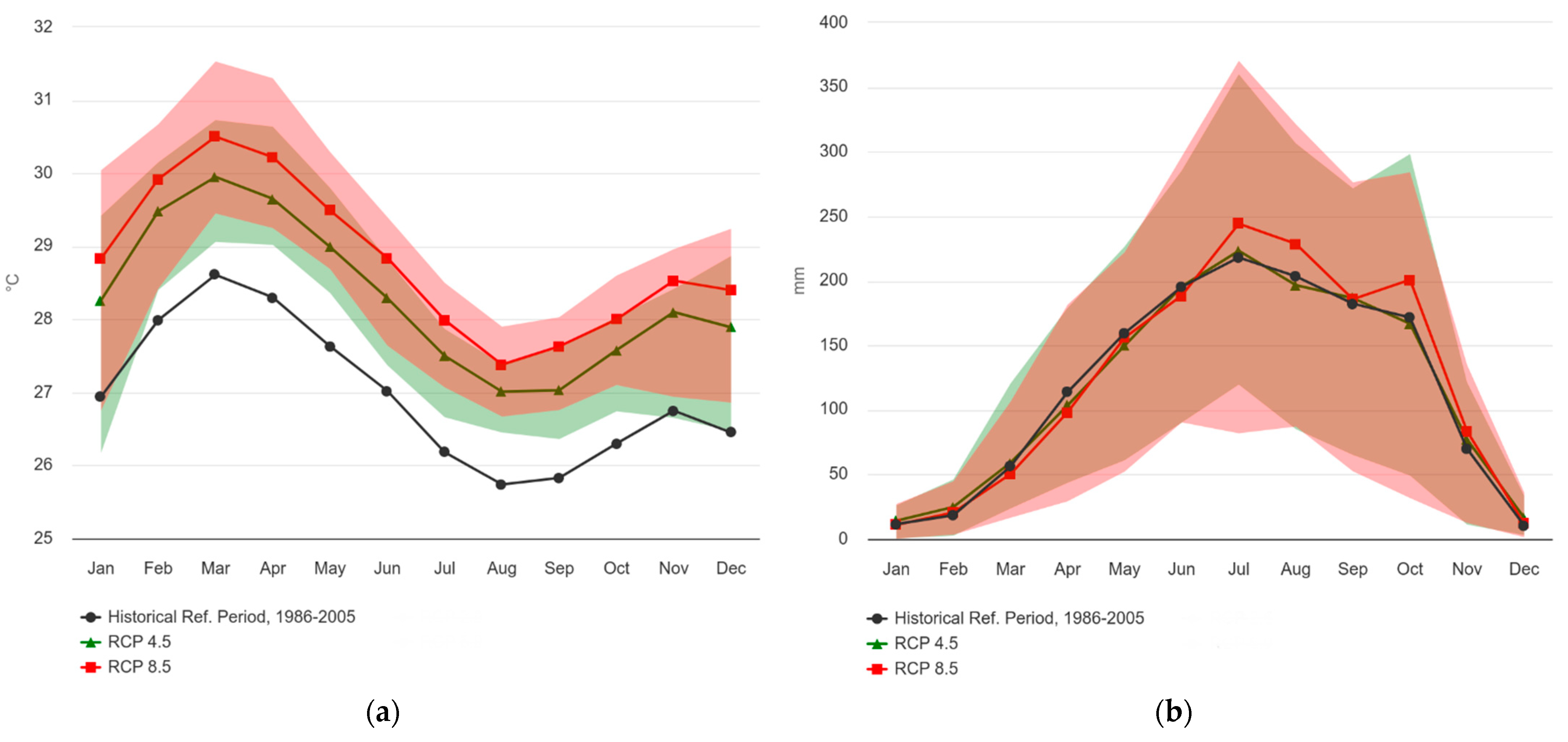
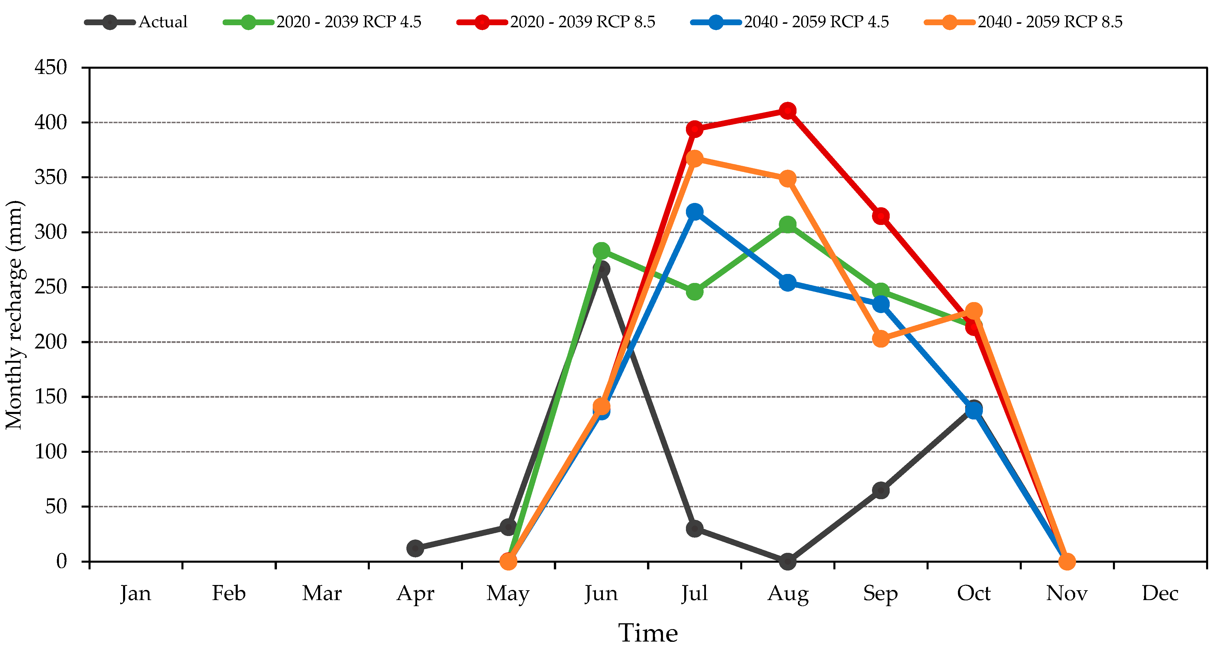
As described above, the Thornthwaite model was used to estimate current and future recharge under the RCP 4.5 and RCP 8.5 scenarios (for the periods 2020–2039 and 2040–2059) in the Togolese coastal sedimentary basin.

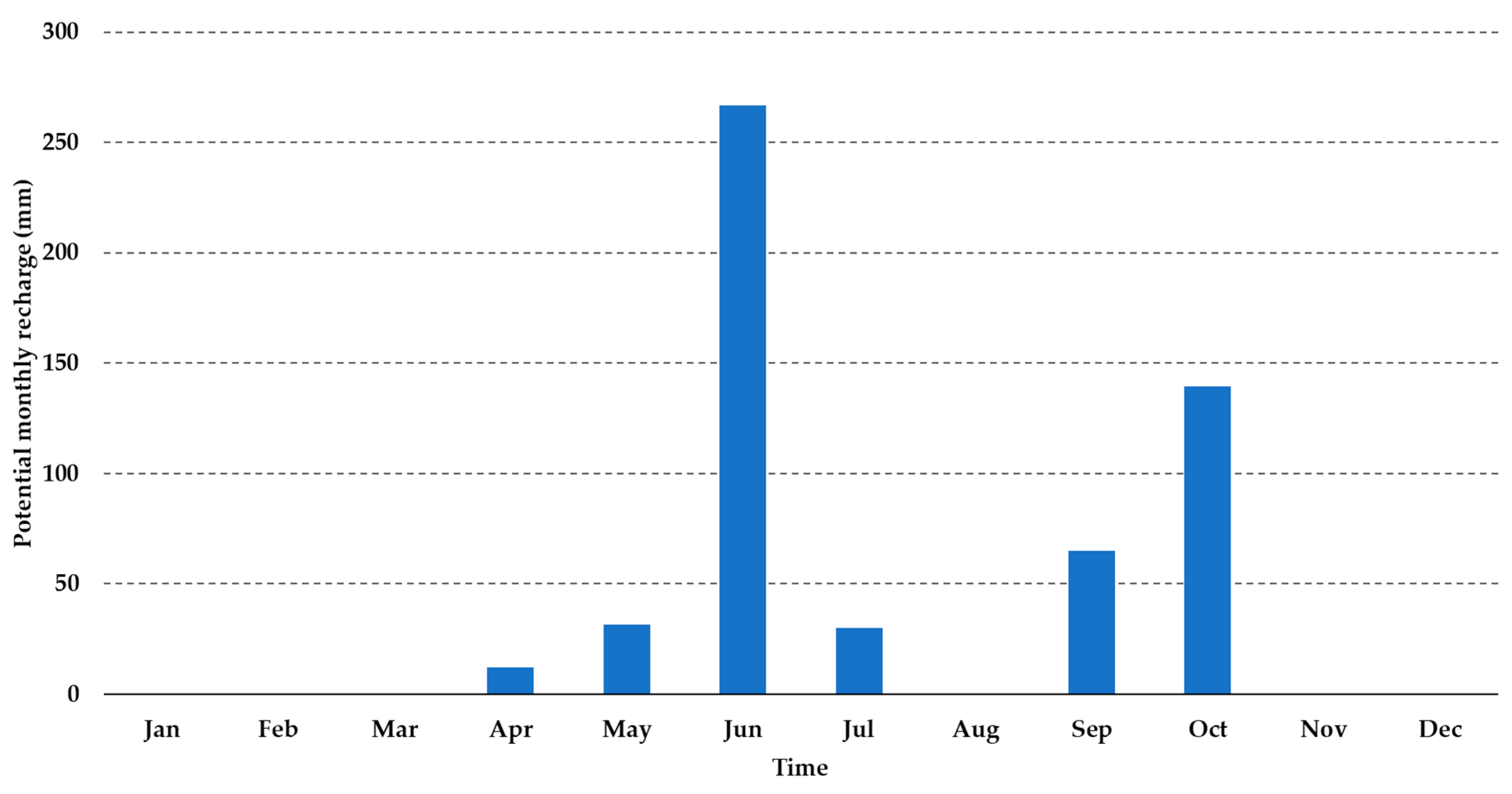
Our results, summarized in Figure 15, show that, in both scenarios, compared to the current period, groundwater recharge increases more under RCP 8.5 than under RCP 4.5. They also demonstrate that, in the future, recharge will occur in a single block, in contrast to the two peaks of recharge currently observed. This is because the groundwater recharge calculated by the Thornthwaite model is directly dependent on rainfall, and in both scenarios the area in which the basin is located will have only one rainy season, as opposed to the two seasons currently observed.

It is not easy to situate the trends observed in this study within major global trends. It can, however, be noted that the Togolese coastal aquifers are not part of the 44% of global aquifers that will experience recharge difficulties due to climate change [51]. Indeed, in a recent global review, Cárdenas Castillero, Kuráž, and Rahim Cárdenas Castillero, Kuráž and Rahim [4] located aquifers that experience decreases in recharge occurring in semi-arid and arid areas, while increases in recharge will be observed in regions where snow predominates in winter and at high altitudes such as the Alps and the Himalayas. Even though the author recognizes that the African continent where the study area is located remains to be studied, a relationship between the recharge and the quantity of water available on the surface in the future may also emerge in Africa. Thus, the regions in which a drop in precipitation is expected—in the Sahel, in North or southern Africa—will experience drops in groundwater recharge [33,58,59,60,61]. On the other hand, in equatorial and tropical regions, recharges are expected to increase due to future increases in precipitation [32,34].

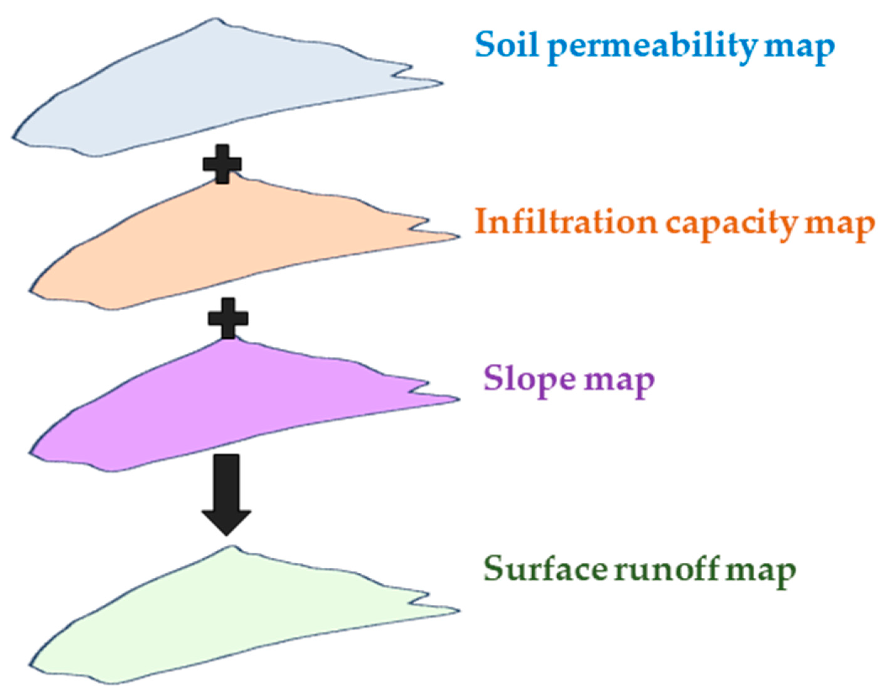
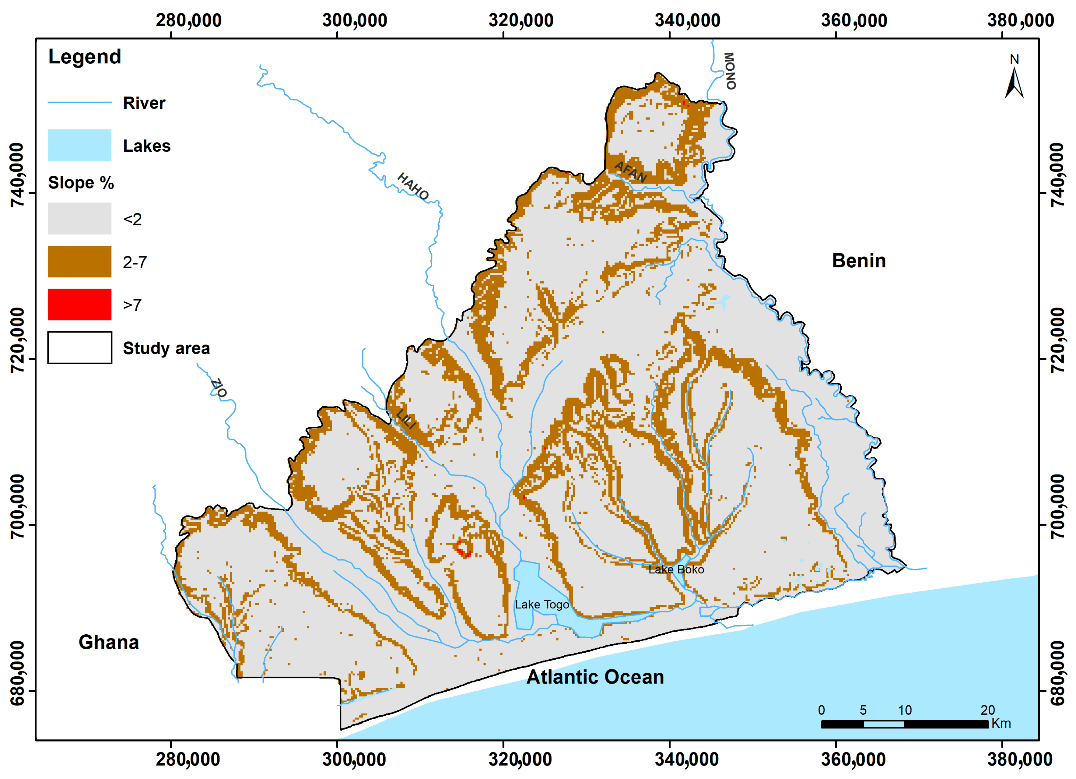
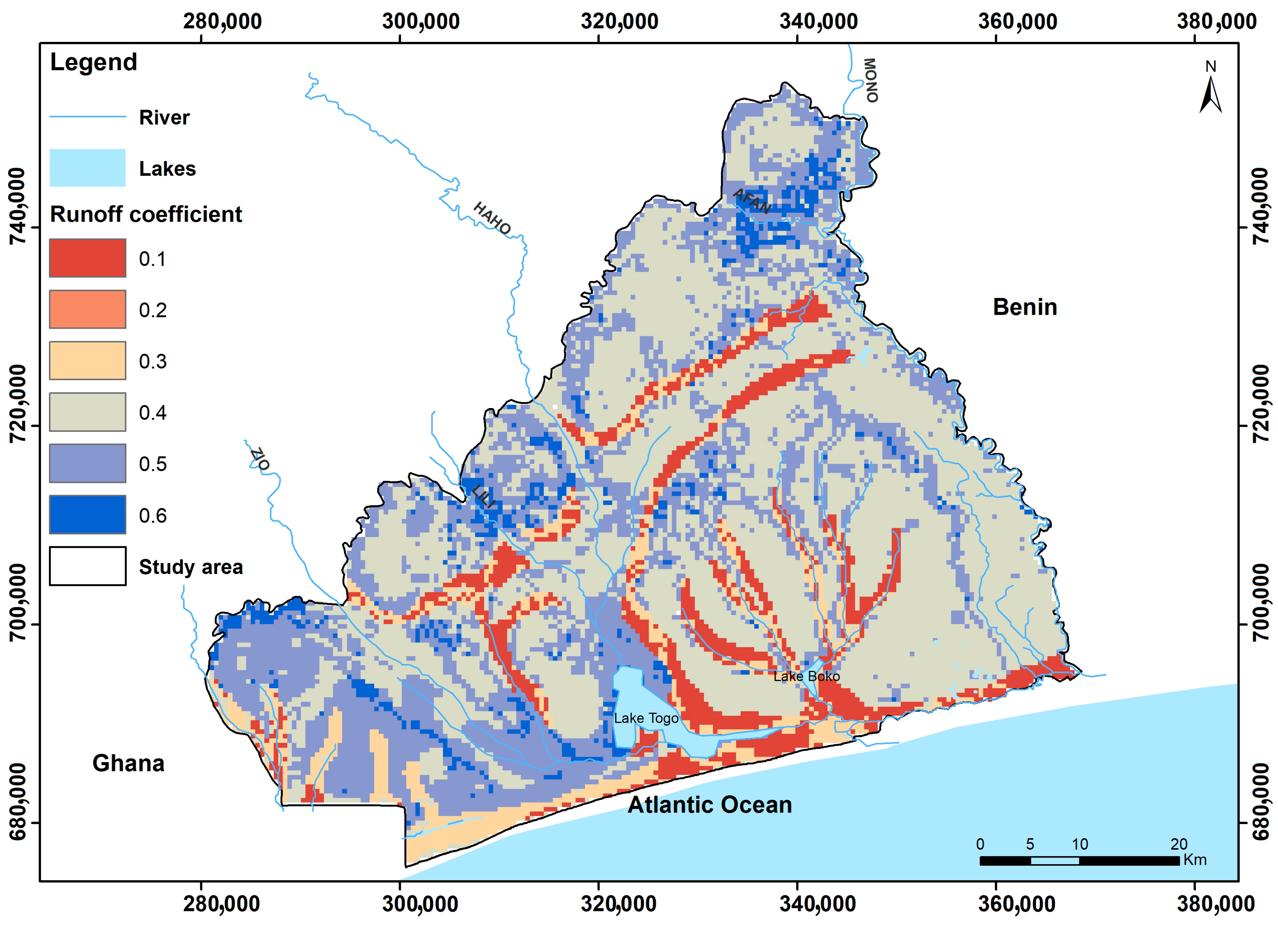
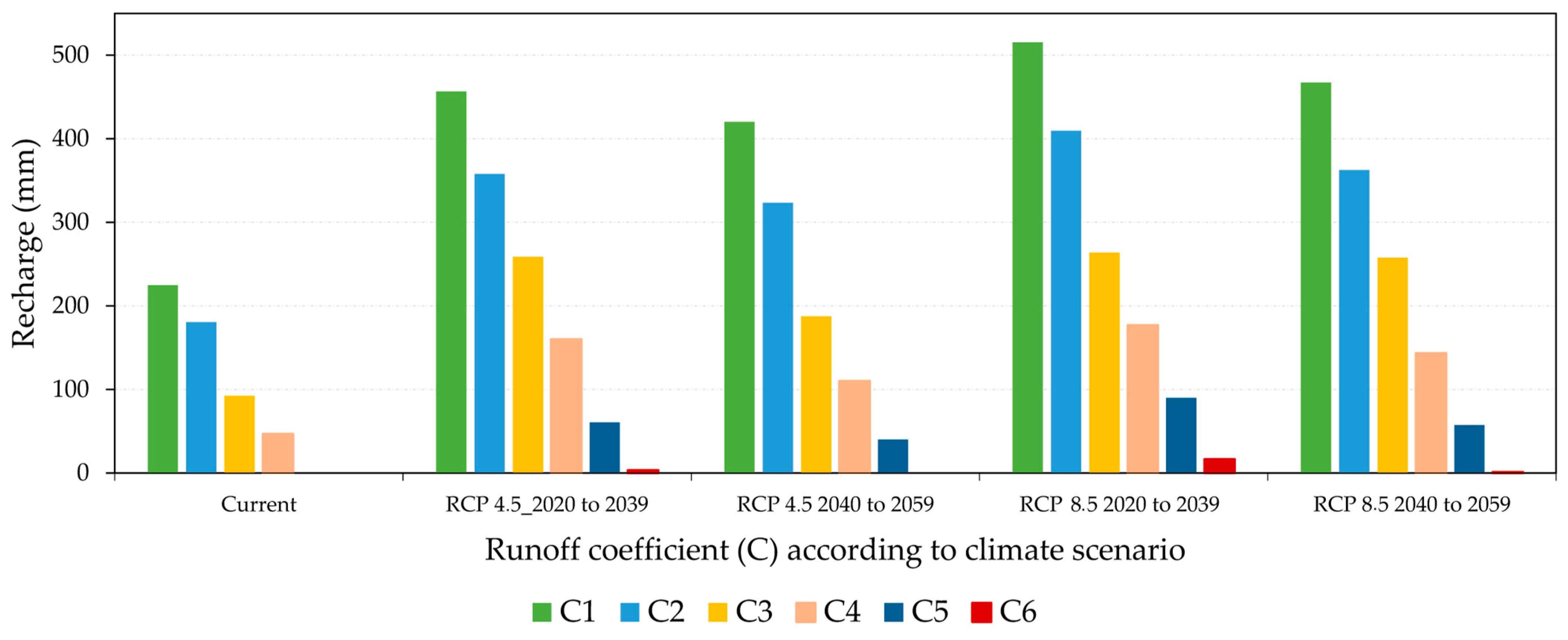
While climate has a significant impact on groundwater recharge, local physical characteristics also play a role. The runoff coefficient, which reflects the impact of slope, soil permeability, and infiltration capacity, serves as an example. As may be seen from Figure 16, the recharge is inversely related to the runoff coefficient value. Whatever the climatic scenario, C₁ = 0.1 is found to have the highest recharge. These are regions with very permeable soils, a mild slope (2%), and forest or savannah vegetation. Therefore, these circumstances favor groundwater recharge. The high runoff zones C₆ = 0.6, which are situated on steep slopes (>7%) and where water does not have time to permeate the soil, are at the other end of the spectrum.

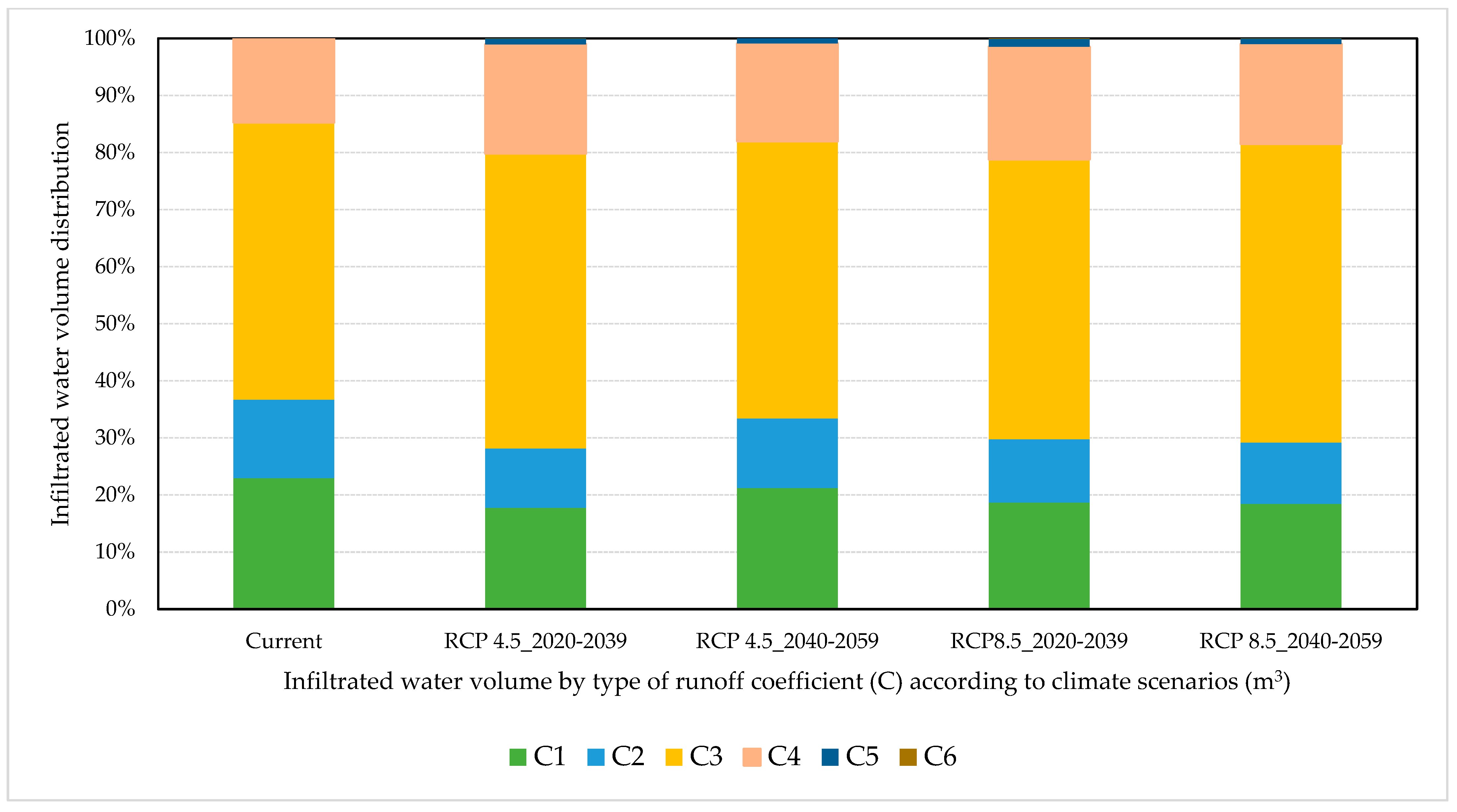
Although, in theory, the runoff coefficient determines the recharge in the basin, the surface area covered by each runoff coefficient will also have an absolute impact on the volume of groundwater that actually reaches the aquifer. Since C3 areas (0.3) constitute a larger portion of the basin’s surface area than C1 areas (0.1), it is clear that these areas experience higher recharge volumes (

Table 9. Recharged volume evolution as a function of runoff coefficient.

	Infiltrated Water Volume (106 m3)
Surface Runoff Coef C	Surface (km2)	Current	RCP 4.5_2020–2039	RCP 4.5_2040–2059	RCP 8.5_2020–2039	RCP 8.5_2040–2059
C1	322.8	72.5	147.4	135.7	166.4	150.8
C2	241.7	43.6	86.5	78.2	99	87.6
C3	1659.2	153.6	429.5	311.2	437.7	427.5
C4	997.1	46.6	159.4	109.9	176.2	142.9
C5	138.3		8.4	5.6	12.5	7.9
C6	28.0		0.09		0.5	0.03

and Figure 17).

It is also critical to remember that we cannot have blind faith in these outcomes. The anticipated intensity of precipitation may result in more runoff than expected, which will lower the anticipated recharge, given the projected increase in extreme events. Therefore, to produce a more accurate estimate of recharge, information on past, present, and projected changes in rainfall intensity will be required. It is precisely the projected increase in rainfall variability, in both intensity and frequency, that, according to Aizebeokhai [87], will most likely result in a reduction in recharge in most of southern Nigeria, a region subject to a climate comparable to that of our study area.

Second, changes in land use can also reduce recharge if soils are sealed or increase expected recharge if developments lead to artificial recharge. Favreau et al. [88] describe an increase in recharge in the Nigerien Sahel due to the type of land use, despite the reduced rainfall observed. On the other hand, even if recharge does occur, it will only supply the unconfined aquifer and the Maastrichtian semi-captive aquifer. The risk of emptying and therefore losing the confined Paleocene aquifer cannot therefore be ruled out.

Finally, a rapid increase in recharge cannot be good news, given that the terminal continental unconfined aquifer is almost outcropping, particularly in the city of Lomé. Groundwater levels could rise significantly in the area, which could cause geotechnical issues and more frequent flooding.

To conclude this section, the results obtained need to be contextualized not as absolute values, but as relative values. Using the methodology adopted, besides considering its own uncertainties related to the water balance, it is necessary to add the many uncertainties related to the climate projections and their scaling [89]. These results therefore provide directions and trends that must be clarified in the future.

5. Conclusions

In this study, the current groundwater recharge and its future evolution under the RCP 4.5 “optimistic” and RCP 8.4 “pessimistic” climate scenarios were estimated in an ungauged basin in the tropics using the Thornthwaite–Mather balance method. In the context of limited data on groundwater, it was a question of estimating the future evolution of recharge and its distribution in space.

The work was based on current temperature and precipitation data observed in the region between 1991 and 2020 and future climate projections for the periods 2020–2039 and 2040–2059. Evapotranspiration was achieved using the Thornthwaite method, and runoff was estimated based on a coefficient that considers the slope, infiltration capacity, and permeability of the soil.

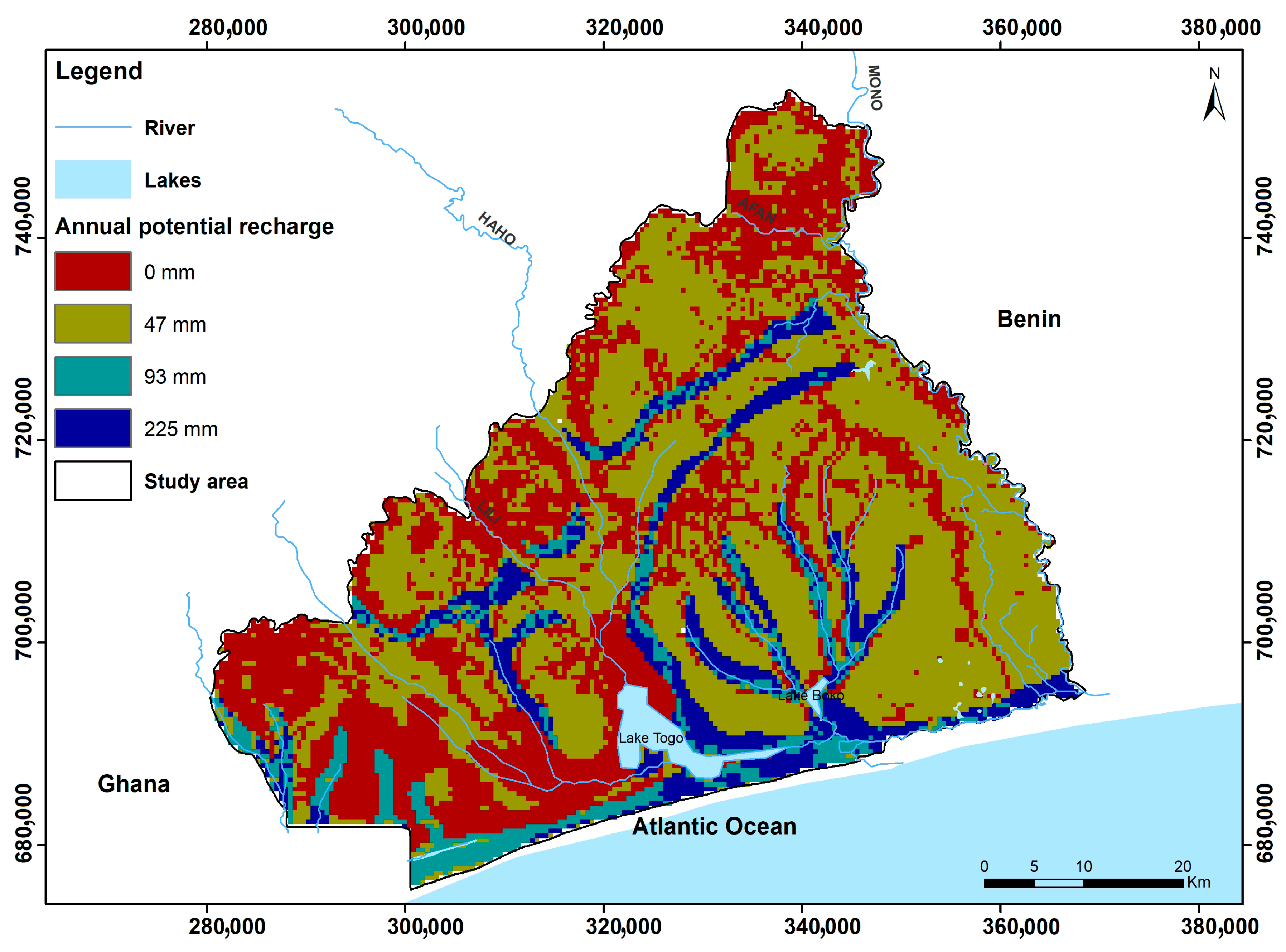
In today’s climate, annual recharge ranges from 47 to 225 mm. The spatial distribution map of the current recharge obtained from the different runoff classes indicated that recharge in the Togolese coastal sedimentary basin depends almost entirely on the nature of the soil. The highest recharge occurs in the sandy deposits along the shoreline and riverbanks. The lowest recharges are in the sandy loam, especially those marked by urbanization and agriculture. The estimate of future recharge is trending upwards. Under the optimistic RCP 4.5 scenario, recharge will be between 3 and over 455 mm per year from 2020 to 2039 and between 40 and 420 mm per year over the period 2040–2059. Under the pessimistic 8.5 scenario, recharge in the basin will be between 16 and 515 mm per year from 2020 to 2049 and between 1 and 467 mm per year over the period 2040–2059.

This study, which is the first to focus on the issue of recharge in the area, illustrates elements of great importance. First, it shows that the recharge in the basin correlated to precipitation will increase. As a result, from a quantitative standpoint, the risk of water scarcity is low if soil artificialization is controlled and withdrawals are reasonable. On the other hand, the study allowed us to identify the preferential zones of groundwater recharge. This offers the possibility to better target the actions to protect the resource from the risk of pollution, but also to guard against the risks linked to a possible excess of water, such as rising water tables. In the context of limited resources, this is valuable information which will be available to local water resource managers. Indeed, if recharge tends to increase in the future, decision makers can consider directing the limited resources available to preserving water quality to make optimal use of them. However, to determine precise answers, efforts are needed to monitor the resource and to manage land cover and waterproofing, and research is needed to better characterize water balance conditions in time and space, such as evapotranspiration, runoff, and soil moisture.

References

1. GIEC. Changements Climatiques 2014: Rapport de Synthèse; Contribution des Groupes de Travail I, II et III au Cinquième Rapport D’évaluation du Groupe D’experts Intergouvernemental sur L’évolution du Climat [Sous la Direction de L’équipe de Rédaction Principale, R.K. Pachauri et L.A. Meyer]; GIEC: Genève, Suisse, 2014; pp. 60–79. [Google Scholar]
2. Oni, S.K.; Futter, M.N.; Molot, L.A.; Dillon, P.J.; Crossman, J. Uncertainty assessments and hydrological implications of climate change in two adjacent agricultural catchments of a rapidly urbanizing watershed. Sci. Total Environ. 2014, 473–474, 326–337. [Google Scholar] [CrossRef] [PubMed]
3. Porporato, A.; Associate Editor: William, F.F.; Daly, E.; Rodriguez-Iturbe, I. Soil Water Balance and Ecosystem Response to Climate Change. Am. Nat. 2004, 164, 625–632. [Google Scholar] [CrossRef] [PubMed]
4. Cárdenas Castillero, G.; Kuráž, M.; Rahim, A. Review of Global Interest and Developments in the Research on Aquifer Recharge and Climate Change: A Bibliometric Approach. Water 2021, 13, 3001. [Google Scholar] [CrossRef]
5. Brouyère, S.; Carabin, G.; Dassargues, A. Climate change impacts on groundwater resources: Modelled deficits in a chalky aquifer, Geer basin, Belgium. Hydrogeol. J. 2003, 12, 123–134. [Google Scholar] [CrossRef]
6. Earman, S.; Dettinger, M. Potential impacts of climate change on groundwater resources—A global review. J. Water Clim. Change 2011, 2, 213–229. [Google Scholar] [CrossRef]
7. Green, T.R. Linking climate change and groundwater. In Integrated Groundwater Management: Concepts, Approaches and Challenges; Jakeman, A.J., Barreteau, O., Hunt, R.J., Rinaudo, J.-D., Ross, A., Eds.; Springer International Publishing: Cham, Switzerland, 2016; pp. 97–141. [Google Scholar]
8. Ranjan, P.; Kazama, S.; Sawamoto, M. Effects of climate change on coastal fresh groundwater resources. Glob. Environ. Chang. 2006, 16, 388–399. [Google Scholar] [CrossRef]
9. Rivera, A.; Allen, D.M.; Maathuis, H. Climate Variability and Change-Groundwater Resources. In Threats to Water Availability in Canada; National Water Research Institute (NWRI): Burlington, ON, Canada, 2004; pp. 77–83. [Google Scholar]
10. Stagl, J.; Mayr, E.; Koch, H.; Hattermann, F.F.; Huang, S. Effects of climate change on the hydrological cycle in Central and Eastern Europe. In Managing Protected Areas in Central and Eastern Europe under Climate Change; Springer: Dordrecht, The Netherlands, 2014; pp. 31–43. [Google Scholar]
11. Erturk, A.; Ekdal, A.; Gurel, M.; Karakaya, N.; Guzel, C.; Gonenc, E. Evaluating the impact of climate change on groundwater resources in a small Mediterranean watershed. Sci. Total Environ. 2014, 499, 437–447. [Google Scholar] [CrossRef] [PubMed]
12. Shrestha, S.; Bhatta, B.; Shrestha, M.; Shrestha, P.K. Integrated assessment of the climate and landuse change impact on hydrology and water quality in the Songkhram River Basin, Thailand. Sci. Total Environ. 2018, 643, 1610–1622. [Google Scholar] [CrossRef]
13. Archer, D.R.; Fowler, H.J. Spatial and temporal variations in precipitation in the Upper Indus Basin, global teleconnections and hydrological implications. Hydrol. Earth Syst. Sci. 2004, 8, 47–61. [Google Scholar] [CrossRef]
14. Collignon, B. Impact des activités humaines sur les ressources en eau souterraine en Afrique sahélienne et soudanienne. In Enregistreurs et Indicateurs de L’évolution de L’environnement en Zone Tropicale; Presses Universitaires de Bordeaux: Pessac, France, 1994; pp. 11–26. [Google Scholar]
15. Richey, A.S.; Thomas, B.F.; Lo, M.H.; Reager, J.T.; Famiglietti, J.S.; Voss, K.; Swenson, S.; Rodell, M. Quantifying renewable groundwater stress with GRACE. Water Resour. Res. 2015, 51, 5217–5238. [Google Scholar] [CrossRef]
16. Konikow, L.F. Long-term groundwater depletion in the United States. Ground Water 2015, 53, 2–9. [Google Scholar] [CrossRef]
17. Lall, U.; Josset, L.; Russo, T. A Snapshot of the World’s Groundwater Challenges. Annu. Rev. Environ. Resour. 2020, 45, 171–194. [Google Scholar] [CrossRef]
18. Brett-Crowther, M.R. Taming the Anarchy: Groundwater Governance in South Asia. Int. J. Environ. Stud. 2009, 66, 818–821. [Google Scholar] [CrossRef]
19. Easter, K.W.; Hearne, R. Book Review: Groundwater Markets and Irrigation Development: Political Economy and Practical Policy. Land Econ. 1995, 71, 261–264. [Google Scholar] [CrossRef]
20. Kumar, R.; Singh, V.P.; Jhajharia, D.; Mirabbasi, R. Agricultural Impacts of Climate Change; CRC Press: Boca Raton, FL, USA, 2019. [Google Scholar] [CrossRef]
21. Dietz, T.; Shwom, R.L.; Whitley, C.T. Climate Change and Society. Annu. Rev. Sociol. 2020, 46, 135–158. [Google Scholar] [CrossRef]
22. Nhamo, G.; Mjimba, V. (Eds.) Sustainability, Climate Change and the Green Economy; Africa Institute of South Africa: Pretoria, South Africa, 2016. [Google Scholar]
23. Subedi, R.C.; Bhuju, D.R.; Bhatta, G.D.; Pant, R.R. Climatic variability and livelihood of rural farmers in Chisapani, Ramechhap, Nepal. Nepal J. Environ. Sci. 2018, 6, 47–59. [Google Scholar] [CrossRef]
24. Giordano, M. Global Groundwater? Issues and Solutions. Annu. Rev. Environ. Resour. 2009, 34, 153–178. [Google Scholar] [CrossRef]
25. Bergkamp, G.; Cross, K. Groundwater and ecosystem services: Towards their sustainable use. In Proceedings of the International Symposium on Groundwater Sustainability; InterAcademy Panel: Alicante, Spain, 2006; pp. 177–193. [Google Scholar]
26. Sophocleous, M. Environmental implications of intensive groundwater use with special regard to streams and wetlands. In Intensive Use of Groundwater: Challenges and Opportunities; Swets & Zeitlinger BV: Lisse, The Netherlands, 2003; pp. 93–112. [Google Scholar]
27. Milly, P.C.; Dunne, K.A.; Vecchia, A.V. Global pattern of trends in streamflow and water availability in a changing climate. Nature 2005, 438, 347–350. [Google Scholar] [CrossRef]
28. Marhaento, H.; Booij, M.J.; Hoekstra, A.Y. Hydrological response to future land-use change and climate change in a tropical catchment. Hydrol. Sci. J. 2018, 63, 1368–1385. [Google Scholar] [CrossRef]
29. Barbieri, M.; Barberio, M.D.; Banzato, F.; Billi, A.; Boschetti, T.; Franchini, S.; Gori, F.; Petitta, M. Climate change and its effect on groundwater quality. Env. Geochem Health 2023, 45, 1133–1144. [Google Scholar] [CrossRef]
30. Epting, J.; Michel, A.; Affolter, A.; Huggenberger, P. Climate change effects on groundwater recharge and temperatures in Swiss alluvial aquifers. J. Hydrol. X 2021, 11, 100071. [Google Scholar] [CrossRef]
31. Sun, Y.; Zhang, W.; Peng, H.; Zhou, F.; Jiang, A.; Chen, X.; Wang, H. The Impacts of Climate Change on the Hydrological Process and Water Quality in the Three Gorges Reservoir Area, China. Water 2023, 15, 1542. [Google Scholar] [CrossRef]
32. Nyenje, P.M.; Batelaan, O. Estimating the effects of climate change on groundwater recharge and baseflow in the upper Ssezibwa catchment, Uganda. Hydrol. Sci. J. 2009, 54, 713–726. [Google Scholar] [CrossRef]
33. Ascott, M.J.; Macdonald, D.M.J.; Sandwidi, W.J.P.; Black, E.; Verhoef, A.; Zongo, G.; Tirogo, J.; Cook, P. Time of emergence of impacts of climate change on groundwater levels in sub-Saharan Africa. J. Hydrol. 2022, 612, 128107. [Google Scholar] [CrossRef]
34. Mileham, L.; Taylor, R.G.; Todd, M.; Tindimugaya, C.; Thompson, J. The impact of climate change on groundwater recharge and runoff in a humid, equatorial catchment: Sensitivity of projections to rainfall intensity. Hydrol. Sci. J. 2009, 54, 727–738. [Google Scholar] [CrossRef]
35. Margat, J.; Van der Gun, J. Groundwater around the World: A Geographic Synopsis; CRC Press: Boca Raton, FL, USA, 2013. [Google Scholar]
36. Sophocleous, M.A. Combining the soilwater balance and water-level fluctuation methods to estimate natural groundwater recharge: Practical aspects. J. Hydrol. 1991, 124, 229–241. [Google Scholar] [CrossRef]
37. Yun, S.-M.; Jeon, H.-T.; Cheong, J.-Y.; Kim, J.; Hamm, S.-Y. Combined Analysis of Net Groundwater Recharge Using Water Budget and Climate Change Scenarios. Water 2023, 15, 571. [Google Scholar] [CrossRef]
38. Seiler, K.-P.; Gat, J.R. Groundwater Recharge from Run-Off, Infiltration and Percolation; Springer Science & Business Media: Berlin/Heidelberg, Germany, 2007; Volume 55. [Google Scholar]
39. Thornthwaite, C.W. An approach toward a rational classification of climate. Geogr. Rev. 1948, 38, 55–94. [Google Scholar] [CrossRef]
40. Kumar, C.P. Estimation of Natural Ground Water Recharge. ISH J. Hydraul. Eng. 1997, 3, 61–74. [Google Scholar] [CrossRef]
41. Barbecot, F.; Guillon, S.; Pili, E.; Larocque, M.; Gibert-Brunet, E.; Hélie, J.-F.; Noret, A.; Plain, C.; Schneider, V.; Mattei, A.; et al. Using Water Stable Isotopes in the Unsaturated Zone to Quantify Recharge in Two Contrasted Infiltration Regimes. Vadose Zone J. 2018, 17, 1–13. [Google Scholar] [CrossRef]
42. Taylor, C.J.; Alley, W.M. Ground-Water-Level Monitoring and the Importance of Long-Term Water-Level Data; US Geological Survey: Denver, CO, USA, 2001; Volume 1217.
43. Albert, T.; Foster, S.; Kemper, K.; Garduno, H.; Nanni, M. Groundwater Monitoring Requirements for Managing Aquifer Response and Quality Threats; The World Bank: Washington, DC, USA, 2004. [Google Scholar]
44. Healy, R.W. Estimating Groundwater Recharge; Cambridge University Press: Cambridge, UK, 2010. [Google Scholar]
45. Galvão, P.; Hirata, R.; Conicelli, B. Estimating groundwater recharge using GIS-based distributed water balance model in an environmental protection area in the city of Sete Lagoas (MG), Brazil. Environ. Earth Sci. 2018, 77, 398. [Google Scholar] [CrossRef]
46. Mattei, A.; Barbecot, F.; Goblet, P.; Guillon, S. Pore water isotope fingerprints to understand the spatiotemporal groundwater recharge variability in ungauged watersheds. Vadose Zone J. 2020, 19, e20066. [Google Scholar] [CrossRef]
47. Thornthwaite, C.W.; Mather, J.R. The water budget and its use in irrigation. In Water: The Yearbook of Agriculture; U. S. Department of Agriculture: Washington, DC, USA, 1955; pp. 346–358. [Google Scholar]
48. Boutt, D.F.; Allen, M.; Settembrino, M.; Bonarigo, A.; Ingari, J.; Demars, R.; Munk, L.A. Groundwater recharge to a structurally complex aquifer system on the island of Tobago (Republic of Trinidad and Tobago). Hydrogeol. J. 2021, 29, 799–818. [Google Scholar] [CrossRef]
49. Carretero, S.; Rodrigues Capítulo, L.; Kruse, E. Evolution of groundwater recharge as a result of forest development on the east coast of the province of Buenos Aires, Argentina. Hydrogeol. J. 2021, 29, 783–797. [Google Scholar] [CrossRef]
50. Carvalho Resende, T.; Longuevergne, L.; Gurdak, J.J.; Leblanc, M.; Favreau, G.; Ansems, N.; Van der Gun, J.; Gaye, C.B.; Aureli, A. Assessment of the impacts of climate variability on total water storage across Africa: Implications for groundwater resources management. Hydrogeol. J. 2018, 27, 493–512. [Google Scholar] [CrossRef]
51. Cuthbert, M.O.; Gleeson, T.; Moosdorf, N.; Befus, K.M.; Schneider, A.; Hartmann, J.; Lehner, B. Global patterns and dynamics of climate–groundwater interactions. Nat. Clim. Chang. 2019, 9, 137–141. [Google Scholar] [CrossRef]
52. Dubois, E.; Larocque, M.; Gagné, S.; Braun, M. Climate Change Impacts on Groundwater Recharge in Cold and Humid Climates: Controlling Processes and Thresholds. Climate 2022, 10, 6. [Google Scholar] [CrossRef]
53. Dubois, E.; Larocque, M.; Gagné, S.; Meyzonnat, G. Simulation of long-term spatiotemporal variations in regional-scale groundwater recharge: Contributions of a water budget approach in cold and humid climates. Hydrol. Earth Syst. Sci. 2021, 25, 6567–6589. [Google Scholar] [CrossRef]
54. Carter, S.-S.A.R.; Bevan, J. Groundwater development for poverty alleviation in sub-Saharan Africa. In Applied Groundwater Studies in Africa; CRC Press: Boca Raton, FL, USA, 2008; pp. 35–52. [Google Scholar]
55. MacDonald, A.M.; Bonsor, H.C.; Dochartaigh, B.É.Ó.; Taylor, R.G. Quantitative maps of groundwater resources in Africa. Environ. Res. Lett. 2012, 7, 024009. [Google Scholar] [CrossRef]
56. Masiyandima, M.; Giordano, M. Sub-Saharan Africa: Opportunistic exploitation. In The Agricultural Groundwater Revolution: Opportunities and Threats to Development; CABI: Wallingford, UK, 2007; pp. 79–99. [Google Scholar]
57. Taylor, R.G.; Koussis, A.D.; Tindimugaya, C. Groundwater and climate in Africa—A review. Hydrol. Sci. J. 2009, 54, 655–664. [Google Scholar] [CrossRef]
58. Kusangaya, S.; Warburton, M.L.; Archer van Garderen, E.; Jewitt, G.P.W. Impacts of climate change on water resources in southern Africa: A review. Phys. Chem. Earth Parts A/B/C 2014, 67–69, 47–54. [Google Scholar] [CrossRef]
59. Dennis, I.; Dennis, R. Climate change vulnerability index for South African aquifers. Water SA 2012, 38, 417–426. [Google Scholar] [CrossRef]
60. Cullis, J.; Strzepek, K.; Tadross, M.; Sami, K.; Havenga, B.; Gildenhuys, B.; Smith, J. Incorporating climate change into water resources planning for the town of Polokwane, South Africa. Clim. Chang. 2010, 108, 437–456. [Google Scholar] [CrossRef]
61. Chikozho, C. Globalizing Integrated Water Resources Management: A Complicated Option in Southern Africa. Water Resour. Manag. 2007, 22, 1241–1257. [Google Scholar] [CrossRef]
62. Barry, R.; Barbecot, F.; Rodriguez, M.; Djongon, A.; Akakpo, W. Urban development and intensive groundwater use in African coastal areas: The case of Lomé urban area in Togo. In Groundwater for Sustainable Livelihoods and Equitable Growth; CRC Press: Boca Raton, FL, USA, 2022; pp. 77–94. [Google Scholar]
63. Adjoussi, P. Changement Climatique Global: Évaluation de L’évolution des Paramètres au Togo; Mémoire de maitrise, Université de Lomé: Lomé, Togo, 2000. [Google Scholar]
64. Akakpo, K.M.; Quensière, J.; Gadal, S. État actuel des occupations du sol le long des cours d’eau au Togo: Etude de cas dans la vallée du Mono. In Proceedings of the Séminaire Theia 2016, Géoinformation Pour les Surfaces Continentales au Service de la Recherche et des Politiques Publiques; Agropolis International Montpellier: Montpellier, France, 2016. [Google Scholar]
65. Kpedenou, K.D.; Boukpessi, T.; Tchamie, T.T.K. Quantification des changements de l’occupation du sol dans la préfecture de Yoto (sud-est Togo) à l’aide de l’imagerie satellitaire Landsat. Rev. Des. Sci. L’environnement 2016, 13, 137–156. [Google Scholar]
66. Johnson, A.K. Le Bassin Côtier à Phosphates du Togo: Maastrichtien-Eocène Moyen. Ph.D. Thesis, Université de Dijon, Dijon, France, 1987. [Google Scholar]
67. Gnazou, M.D.T.; Sabi, B.E.; Lavalade, J.L.; Schwartz, J.; Akakpo, W.; Tozo, A. Multilayered aquifer modeling in the coastal sedimentary basin of Togo. J. Afr. Earth Sci. 2017, 125, 42–58. [Google Scholar] [CrossRef]
68. DHE. Surveillance Piezométrique et Chimique des Nappes du Bassin Sédimentaire Côtier du Togo- Synthese des Connaissances Hydrogéologiques; Direction de l’Hydraulique et de l’Energie (DGE): Lomé, Togo, 1982. [Google Scholar]
69. Akouvi, A.; Dray, M.; Violette, S.; de Marsily, G.; Zuppi, G.M. The sedimentary coastal basin of Togo: Example of a multilayered aquifer still influenced by a palaeo-seawater intrusion. Hydrogeol. J. 2008, 16, 419–436. [Google Scholar] [CrossRef]
70. Akouvi, A. Etude Géochimique et Hydrogéologique des Eaux Souterraines d’un Bassin Sedimentaire Cotier en Zone Tropicale. Ph.D. Thesis, University Paris VI, Paris, Frace, 2001. [Google Scholar]
71. Lamouroux, R. Carte pédologique du togo. In Office de la Recherche cientifique et Technique Outre-Mer (ORSTOM); Institut de Recherche et Développement (IRD): Marseille, France, 1960. [Google Scholar]
72. Avumadi, A. Dynamique des Apports Fluviaux Dissous et Particuliaires au lac Togo: Bilans, Origines et Devenir, Mécanismes et Facteurs de Contrôle; Institut National Polytechnique de Toulouse (INPT): Toulouse, France, 2019. [Google Scholar]
73. CCKP. Observed Climatology of Mean-Temperature 1991–2020 Togo. Available online: https://climateknowledgeportal.worldbank.org/country/togo/climate-data-historical (accessed on 20 July 2022).
74. CCKP. Observed Climatology of Precipitation 1991–2020 Togo. Available online: https://climateknowledgeportal.worldbank.org/country/togo/climate-data-historical (accessed on 20 July 2022).
75. Thornthwaite, C.W.; Mather, J.R. Instructions and Tables for Computing Potential Evapotranspiration and the Water Balance; Drexel Institue of Technology Laboratory of Climatology: Centerton, NJ, USA, 1957. [Google Scholar]
76. CCKP. Climate Change Knowledge Portal The Climate Change Knowledge Portal (CCKP). Available online: https://www.worldbank.org/en/about/legal (accessed on 20 July 2022).
77. USGS. Shuttle Radar Topography Mission (SRTM). In USGS EROS Archive—Digital Elevation—Shuttle Radar Topography Mission (SRTM); United States Geological Survey (USGS): Sioux Falls, SD, USA, 2021. [Google Scholar]
78. Friedl, M.; Sulla-Menashe, D. MCD12Q1 MODIS/Terra+Aqua Land Cover Type Yearly L3 Global 500m SIN Grid V006. Available online: https://lpdaacsvc.cr.usgs.gov/appeears/help (accessed on 20 July 2022).
79. Koerner, R.M.; Daniel, D.E. Final Covers for Solid Waste Landfills and Abandoned Dumps; Thomas Telford: London, UK, 1997. [Google Scholar]
80. Totin, V.S.H. Assessment of Global Change Impacts on Groundwater in the Coastal Sedimentary Basin of Benin (West Africa); Global Change SysTem for Analysis, Research and Training (START): Washington, DC, USA, 2009. [Google Scholar]
81. Koudjega, K.H.; Kodja, D.J.; Vissin, W.E. Evaluation de la Recharge des Eaux Souterraines Profonde de l’Aquifère du Paléocène Supérieure dans le Bassin du Mono-Couffo au Benin. Int. J. Progress. Sci. Technol. 2020, 20, 11. [Google Scholar]
82. Task Force on Effect of Urban Development on Flood Discharges. Effect of Urban Development on Flood Discharge-Current Knowledge and Future-Needs. J. Hydrau. Div. 1969, 95, 287–310. [Google Scholar] [CrossRef]
83. Taylor, K.E.; Stouffer, R.J.; Meehl, G.A. An overview of CMIP5 and the experiment design. Bull. Am. Meteorol. Soc. 2012, 93, 485–498. [Google Scholar] [CrossRef]
84. CCKP. Climate Projections CMIP5 Data, Togo. Available online: https://climateknowledgeportal.worldbank.org/country/togo/cmip5 (accessed on 20 July 2022).
85. Thomson, A.M.; Calvin, K.V.; Smith, S.J.; Kyle, G.P.; Volke, A.; Patel, P.; Delgado-Arias, S.; Bond-Lamberty, B.; Wise, M.A.; Clarke, L.E. RCP4. 5: A pathway for stabilization of radiative forcing by 2100. Clim. Chang. 2011, 109, 77–94. [Google Scholar] [CrossRef]
86. Riahi, K.; Rao, S.; Krey, V.; Cho, C.; Chirkov, V.; Fischer, G.; Kindermann, G.; Nakicenovic, N.; Rafaj, P. RCP 8.5—A scenario of comparatively high greenhouse gas emissions. Clim. Chang. 2011, 109, 33–57. [Google Scholar] [CrossRef]
87. Aizebeokhai, A. Potential impacts of climate change and variability on groundwater resources in Nigeria. Afr. J. Environ. Sci. Technol. 2011, 5, 760–768. [Google Scholar] [CrossRef]
88. Favreau, G.; Cappelaere, B.; Massuel, S.; Leblanc, M.; Boucher, M.; Boulain, N.; Leduc, C. Land clearing, climate variability, and water resources increase in semiarid southwest Niger: A review. Water Resour. Res. 2009, 45. [Google Scholar] [CrossRef]
89. Aslam, R.A.; Shrestha, S.; Pandey, V.P. Groundwater vulnerability to climate change: A review of the assessment methodology. Sci. Total Environ. 2018, 612, 853–875. [Google Scholar] [CrossRef]
Figure 1. Location of the study area.
Water 16 00731 g001
Figure 2. Geomorphological units of the coastal sedimentary basin in Togo and limits of Lomé (adapted from DHE [68]).
Water 16 00731 g002
Figure 3. Transverse N-S geological cross-sections (a), as reported in Figure 2 from DHE [68].
Water 16 00731 g003
Figure 4. Monthly climatology of min temperature, mean temperature, max temperature, and precipitation for 1991–2020 in the maritime region, Togo [73,74].
Water 16 00731 g004
Figure 5. Surface runoff map design method.
Water 16 00731 g005
Figure 7. (a) Projected climatology of mean temperature for the 2020–2039 maritime region of Togo; (Reference Period: 1986–2005). RCP 4.5 and RCP 8.5. Multi-Model Ensemble; (b) projected climatology of precipitation for the 2020–2039 maritime region of Togo; (Reference Period: 1986–2005). RCP 4.5 and RCP 8.5. Multi-Model Ensemble [84].
Water 16 00731 g007
Figure 8. (a) Projected climatology of mean temperature for the 2040–2059 maritime region of Togo; (Reference Period: 1986–2005). RCP 4.5 and RCP 8.5. Multi-Model Ensemble; (b) projected climatology of precipitation for the 2040–2059 maritime region of Togo; (Reference Period: 1986–2005). RCP 4.5 and RCP 8.5. Multi-Model Ensemble [84].
Water 16 00731 g008
Figure 9. Soil (permeability) map.
Water 16 00731 g009
Figure 10. Land cover map.
Water 16 00731 g010
Figure 11. Slope map.
Water 16 00731 g011
Figure 12. Runoff coefficient map.
Water 16 00731 g012
Figure 13. Annual distribution of current groundwater recharge.
Water 16 00731 g013
Figure 14. Current groundwater recharge distribution map.
Water 16 00731 g014
Figure 15. Groundwater recharge evolution in the Togolese coastal sedimentary basin.
Water 16 00731 g015
Figure 16. Recharge evolution according to runoff coefficient in the Togolese coastal sedimentary basin.
Water 16 00731 g016
Figure 17. Recharge evolution according to volumes infiltrated in the Togolese coastal sedimentary basin.
Water 16 00731 g017