Article

Dissolved Oxygen Forecasting for Lake Erie’s Central Basin Using Hybrid Long Short-Term Memory and Gated Recurrent Unit Networks

1
School of Engineering, University of Guelph, 50 Stone Road East, Guelph, ON N1G 2W1, Canada
2
Lakes Environmental, 170 Columbia St. W, Waterloo, ON N2L 3L3, Canada
*
Authors to whom correspondence should be addressed.
Water 2024, 16(5), 707; https://doi.org/10.3390/w16050707
Submission received: 13 January 2024 / Revised: 23 February 2024 / Accepted: 25 February 2024 / Published: 28 February 2024
(This article belongs to the Special Issue Water Quality, Ecological Health and Ecosystem Restoration)

Abstract

:
Dissolved oxygen (DO) concentration is a pivotal determinant of water quality in freshwater lake ecosystems. However, rapid population growth and discharge of polluted wastewater, urban stormwater runoff, and agricultural non-point source pollution runoff have triggered a significant decline in DO levels in Lake Erie and other freshwater lakes located in populated temperate regions of the globe. Over eleven million people rely on Lake Erie, which has been adversely impacted by anthropogenic stressors resulting in deficient DO concentrations near the bottom of Lake Erie’s Central Basin for extended periods. In the past, hybrid long short-term memory (LSTM) models have been successfully used for the time-series forecasting of water quality in rivers and ponds. However, the prediction errors tend to grow significantly with the forecasting period. Therefore, this research aimed to improve the accuracy of DO forecasting models by taking advantage of Lake Erie’s real-time water quality (water temperature and DO concentration) monitoring network to establish temporal and spatial links between adjacent monitoring stations. We developed hybrid LSTM models that combine LSTM, convolutional neuron network LSTM (CNN-LSTM), hybrid CNN with gated recurrent unit (CNN-GRU) models, and convolutional LSTM (ConvLSTM) to forecast near-bottom DO concentrations in Lake Erie’s Central Basin. These hybrid LSTM models improve their capacity to handle complicated datasets with spatial and temporal variability. These models can serve as accurate and reliable tools for forecasting DO concentrations in freshwater lakes to help environmental protection agencies better access and manage the health of these vital ecosystems. Following analysis of a 21-site Lake Erie dataset for 2020 and 2021, the ConvLSTM model emerged as the most accurate and reliable, boasting an MSE of 0.51 mg/L, MAE of 0.42 mg/L, and an R-squared of 0.95 over the 12 h prediction range. The model foresees future hypoxia in Lake Erie. Notably, the temperature near site 713 holds significance for Central Basin DO forecasting in Lake Erie, as indicated by outcomes derived from the Shapley additive explanations (SHAP).

1. Introduction

Dissolved oxygen (DO) is essential for sustaining aquatic life, including maintaining the well-being of fish and benthic communities [1,2,3,4]. Seasonal fluctuations in DO levels, where the minimum DO concentrations drop below 2 mg/L for extended periods, can significantly disrupt aquatic ecosystems. Recent studies emphasize the need to better understand and more accurately forecast DO concentrations, which are crucial for maintaining ecological balance and mitigating long-term environmental changes. DO levels below 4 mg/L are detrimental to fish populations, with further decreases leading to a marked decline in aquatic biodiversity. Extreme cases of hypoxia, where DO falls below 2 mg/L, signal severe ecological distress [1,2,3,4,5,6].
Recognizing the imperative significance of DO, the determination of its concentration emerges as a necessity. A research endeavor delved into the DO concentrations across temperate lakes between latitudes 23.5° and 60° both north and south. The findings revealed a concerning reduction in DO levels, specifically a decline of 5.5% in surface water and a more substantial decrease of 18.6% in the deeper layers of the lake [7]. These outcomes serve as a clear signal for governments and the relevant authorities to take concerted action to safeguard and revitalize the water ecosystem.
Lake Erie, one of the largest freshwater lakes in a temperate region with over 25 thousand square kilometers of surface area, is a hub of ecological diversity and economic activity, housing a rich array of 107 different fish species and supporting over 11 million people. Its fertile surrounding lands and temperate climate fuel thriving agriculture, while its industrial and commercial sectors bolster the regional economy [8]. However, this vibrant freshwater ecosystem faces challenges. Historical eutrophication from runoff and pollution led to detrimental algal blooms, affecting water quality and oxygen levels. Recent studies on Lake Erie have shown the prominent role that DO plays in the dynamics of Lake Erie’s benthic community [1,8,9]. These studies identify hypoxia, or low levels of DO, as a major factor influencing the composition and health of benthic communities, especially in the central basin of Lake Erie [1,9].
Considering these pressing concerns, the practice of DO forecasting emerges as a valuable tool that empowers professionals to make informed decisions. Well-informed recommendations and strategies can be developed to mitigate potential challenges by extrapolating and analyzing future data trends. In a temperate region such as Lake Erie, the specter of decreasing DO levels looms large. It necessitates proactive measures.

1.1. The DO Prediction Models and Previous Work

The forecasting of DO concentration is a focal point within the realm of water quality assessment. This dynamic field has witnessed the application of diverse algorithms, ranging from intricate mathematical fusion models to the robust capabilities of machine learning techniques. Among the arsenal of predictive tools, machine learning models have garnered widespread acclaim for their efficacy in forecasting DO concentration trends [10,11,12,13,14,15,16]. Deep learning has been successfully used to improve DO concentration prediction accuracy in rivers and reservoirs [17,18,19].
Li et al. in 2021 revealed an enhanced predictive method by integrating the support vector regression (SVR) model with various complex metaheuristic algorithms. This innovative amalgamation encompassed the adaptive and nature-inspired Chicken Swarm Optimization, the collaborative and socially driven dynamics of Social Ski-Driver Optimization, the sophisticated and predatory allure of Black Widow Optimization, and the cutting-edge prowess of the Algorithm of the Innovative Gunner. Specifically, a remarkably low root mean square error (RMSE) of 0.644 mg/L attested to its precision, while a determination coefficient ( R 2 ) value of 0.963 was achieved. This prowess became even more pronounced when juxtaposed against the solitary SVR model, revealing a remarkable enhancement in accuracy ranging from 6.52% to 1.75% [20]. However, even amidst the triumphant achievement of this advanced model, it is prudent to acknowledge the inherent complexity it embodies.
In the realm of DO prediction, the year 2020 witnessed a notable contribution by Li et al. [21], who embarked on an insightful exploration of the maximal information coefficient-SVR (MIC-SVR) approach. The fruits of their labor bore witness to a robust model, as evidenced by an RMSE of 3.01%, an impressive Nash–Sutcliffe efficiency (NSE) of 62.36%, and a R 2 of 0.9, outperforming the conventional SVR approach. However, SVR and MIC-SVR are inherently tethered to their decision functions, limiting their capacity to unveil deeper insights, such as the intricate temporal interplay between time and DO concentration.
Zhu et al. contributed a seminal paper that delved into the realm of DO prediction, explicitly focusing on the urban rivers surrounding the Three Gorges Reservoir [22]. Their investigation took an innovative avenue by harnessing the extreme learning machine’s (ELM’s) capabilities and the intricate dynamics of an artificial neural network (ANN). By synergizing these methodologies, they endeavored to unravel the complexities of DO levels within city river systems. Their evaluative arsenal encompassed the RMSE, the mean absolute error (MAE), the R 2 , and the Willmott Index of Agreement.
However, even with the resounding success of their study, certain limitations of machine learning methods cast a shadow upon their accuracy and reliability. These methodologies grapple with the challenge of capturing the intricate interplay of anthropogenic influences, particularly those stemming from changing environmental factors.
Within a study in 2021, the Attention-Gated Recurrent Unit-Gradient Boosting Regression Tree (Attention-GRU-GBRT) emerged as a potent tool for forecasting DO concentrations in pond culture environments. The results reverberated with clarity, showcasing the preeminence of the Attention-GRU-GBRT model with strikingly low MSE, MAE, and RMSE scores of 0.121, 0.219, and 0.348, respectively. However, Cao’s model was tested and optimized within the confines of a specific pond [23]. The heterogeneity of DO variations in deeper systems remains a challenge that could offer deeper insights into the complex interplay of factors shaping DO levels.
Data fusion algorithms have demonstrated significant success in this study. The employed algorithms include the collection of dissolved oxygen (DO) datasets, utilizing the Sparrow Search Algorithm for feature extraction. Subsequently, Attention-GRU was employed for both dataset prediction and interpretation [23]. This methodology effectively integrates optimization algorithms with deep learning, showcasing exceptional predictive capabilities, and can be widely applied in various watersheds.
The long short-term memory (LSTM) model [24], a derivative of recurrent neural networks (RNNs) [25,26], has proven effective in handling data with long-term dependencies, making it highly capable of capturing information. In recent years, research into time-series water quality prediction using LSTM-based models has gained momentum [27,28,29,30,31,32,33,34]. Kim et al. [35] examined various methods for 24 h DO prediction, discovering that LSTM models outperformed traditional machine learning approaches like support vector machines regarding precision and applicability.
Many researchers have come up with methods for forecasting the DO in water. In Cao’s paper, the K-means clustering method predicts the DO and water quality. In their research, their approach provides better performance and higher accuracy compared with PCA-CNN (principal component analysis–convolutional neural network), PCA-LSTM, and PCA-ELM models [36]. However, the authors mainly focus on ponds, with a simple and constant external environment. Lakes have more factors that influence the DO and more complex ecosystems. Thus, there are doubts that K-means models cannot fit the variable environments.
Meanwhile, another paper was published in 2020 [37]. This paper compared four models, including LSTM, ELM, Hammerstein–Weiner, and general regression neural network (GRNN). According to their paper, the four methods had their advantages. The paper proved that these four methods were successfully applied in DO forecasting. However, the four methods were used to analyze availability only. Making the performance better should be investigated in further work.
Zhu et al. [38] introduced a DO forecasting model that improves low DO scenario accuracy by refining the loss function used in LSTM backpropagation. Using the sine function, they adjusted the network weights by assigning different weights to DO at different content levels. In another study, Zhu et al. [39] developed a DO prediction model utilizing advanced deep learning techniques like ResNets, BiLSTM, and attention, highlighting the effectiveness of LSTM as a neural network framework in DO forecasting.
Convolutional neural networks (CNNs) [40,41], a crucial branch of deep learning models, possess strong sequence feature extraction capabilities, effectively modeling long-term dependencies between data points. As a result, more and more researchers have introduced CNNs into hydrology research. Khosravi et al. [42] used a CNN to create a flood risk map in Iran. Chen et al. [43] devised an advanced CNN model to quantitatively analyze water pollution using near-infrared data. Yan et al. [44] applied a one-dimensional residual CNN for water quality prediction. Barzegar et al. [45,46] improved water level and quality predictions with a CNN-LSTM hybrid model. Baek et al. [47] employed a combined CNN-LSTM approach for forecasting water level and quality. In 2021, Yang et al. [48] introduced a CNN-LSTM water quality prediction model that employed two convolutional layers for feature extraction. After processing the time-series data through two LSTM units, an attention mechanism was used to assign weights to the time-series features. As of 2024, the CNN-LSTM model developed by Hu continues to offer a highly efficient method for forecasting dissolved oxygen (DO) [49].
When analyzing data from multiple monitoring stations, analyzing both temporal relationships and spatial trends in data sources is crucial [50]. Convolutional LSTM (ConvLSTM) [51] is a recurrent neural network variant designed to effectively analyze both temporal dynamics and spatial patterns. It integrates convolutional mechanisms into input-to-state and state-to-state transitions, theoretically suitable for DO prediction in different stations across time and space sequences. However, there has been limited research in this area prior to this study.
In a paper published in 2021, the researchers applied three different artificial intelligence models to predict DO concentration in Fanno Creek [52]. The three models discussed are the Deep Recurrent Neural Network (DRNN), SVM, and ANN models. According to their results, the DRNN models performed the best in these three models. The root mean square error (RMSE) was 0.43, and NSE was 0.948. To enhance the performance of artificial neural networks (ANNs), a combination of biogeography-based optimization (BBO) and atom search optimization (ASO) has been employed [53]. Yang applied a similar concept of integrating optimization techniques with artificial neural networks (ANNs). He explored the combination of four optimization methods with a multi-layer perceptron neural network (MLPNN). According to his research findings, the electromagnetic field optimization–MLPNN exhibited the best performance among the tested combinations [50].
Ayesha Jasmin et al. employed the random forest (RF) algorithm to forecast dissolved oxygen (DO) in a shrimp culture system [54]. Despite its simplicity, RF demonstrated strong performance in DO prediction, achieving an R 2 of 0.709, 98.26% accuracy, and a score of 0.7381 [54,55]. Ahmed and Lin published a paper that uses quantile regression forest (QRF) to predict the DO concentration in running water. They forecasted three rivers using QRF, a better RF model. According to their paper, the QRF model can obtain the mean value of DO concentration and give a prediction under defined percentiles. The QRF model is a simple model that allows users to have low related professed knowledge. Their model demonstrates superior performance compared to the multi-layer perceptron neural network and models developed by the U.S. Environmental Protection Agency. The temperature and pH change are the main reasons for the DO change [16]. However, there are still some drawbacks to their model. This model cannot predict the DO concentration outside of training data.
Another paper in 2021 compared three different deep learning methods to forecast the DO levels in the fishery ponds. In their paper, the three methods analyzed were RNN, LSTM, and gated recurrent unit (GRU). The MAE, MSE, mean absolute percentage error (MAPE), and the R 2 were used to determine the performance of the three methods. Based on the result, the GRU method with 0.450 mg/L for MAE, 0.411 for MSE, 0.054 MAPE, and 0.994 for R 2 , respectively, showed the best performance of the three methods [20]. Therefore, the GRU is suitable for fishery pond applications. However, DO for different situations needs to be measured using other methods.
According to the paper of Roushangar et al., a novel model combining LSTM networks and the Satin Bowerbird optimizer (SBO) algorithm is used to predict the DO in the Savannah River, USA. Their advanced model achieves a high performance with a R 2 of 0.981, NSE of 0.957, and RMSE of 0.034. This is evidence that this model performs better than SVM and Gaussian process regression [56]. However, the SBO-LSTM model is complex, leading to a longer running time than other simple models.

1.2. Motivations and Contributions of the Study

Hence, the overarching aim of this paper is to contribute to the arsenal of solutions by identifying and advocating for effective DO prediction methodologies. This study enables stakeholders to anticipate and respond to fluctuations in DO concentration with a higher degree of accuracy. To achieve the primary objective of this study, we have created hybrid LSTM models that combine LSTM, CNN-LSTM, and ConvLSTM to forecast DO in Lake Erie. These hybrid LSTM models improve their capacity to handle complicated datasets while simplifying structural features [57,58,59]. Meanwhile, the hybrid GRU models (GRU and CNN-GRU) are also applied as the comparison models. It is crucial to make several modifications to achieve the intended objective.
In this study, LSTM and GRU models are the basic models used for forecasting DO in Lake Erie. The contributions of the study are summarized in three aspects. First, this study is innovative in employing five models for forecasting the DO concentration of Lake Erie. CNN-GRU and ConvLSTM models demonstrate proficiency in handling data imbued with spatial and temporal characteristics. Secondly, several factors, such as overturning events, introduce complexities in predicting DO. Mere hyperparameter adjustments fall short of mitigating overfitting concerns. This research incorporates regularization techniques to avoid overfitting the model during the training phase. Specifically, the combination of ridge regularization with hybrid LSTM and GRU models effectively addresses overfitting challenges. Finally, this study extends its scope beyond forecasting, delving into analyzing hypoxia trends. Lake Erie has grappled with hypoxia concerns for numerous years, making it a pivotal objective of this study to ascertain alterations in the hypoxic areas using forecasting results.

2. Proposed Approaches

To analyze DO concentration, this paper employs five distinct models: the LSTM, ConvLSTM, CNN-LSTM, GRU, and CNN-GRU models. These models were evaluated for their performance using identical Lake Erie dataset conditions. Furthermore, this paper leveraged various statistical indices to gauge and assess the efficacy of these models.

2.1. Data Background and Analysis

Typically, the uppermost layer of a lake exhibits higher DO levels due to its closer proximity to the atmosphere, which facilitates greater oxygen dissolution into the lake water. Conversely, the deeper layers consistently demonstrate lower DO concentrations, primarily attributable to reduced exposure to surface contact. Notably, aquatic vegetation in the lakebed contributes to oxygen enrichment in the water, as established by previous studies [60,61].
The United States Geological Survey compiled the dataset utilized in our study, USGS Lake Erie Biological Station, which included near-bottom water temperature measurements and DO for the Central Basin of Lake Erie. This dataset covered two distinct periods, from 19 June to 11 October 2020 and from 19 June to 11 October 2021, as documented in [62]. There are 21 water quality monitoring sites in Lake Erie’s Central Basin, as shown in Figure 1. The longitude and latitude information of the 21 sites are shown in Table 1.
We identified three key attributes to serve as the basis for prediction. These attributes consist of date–time stamps, temperature readings, and DO concentrations, each corresponding to all 21 sites, denoted as sites 1007 to 616 in Figure 1. Notably, the data collection process entailed simultaneously recording time and temperature and collecting DO concentration values.
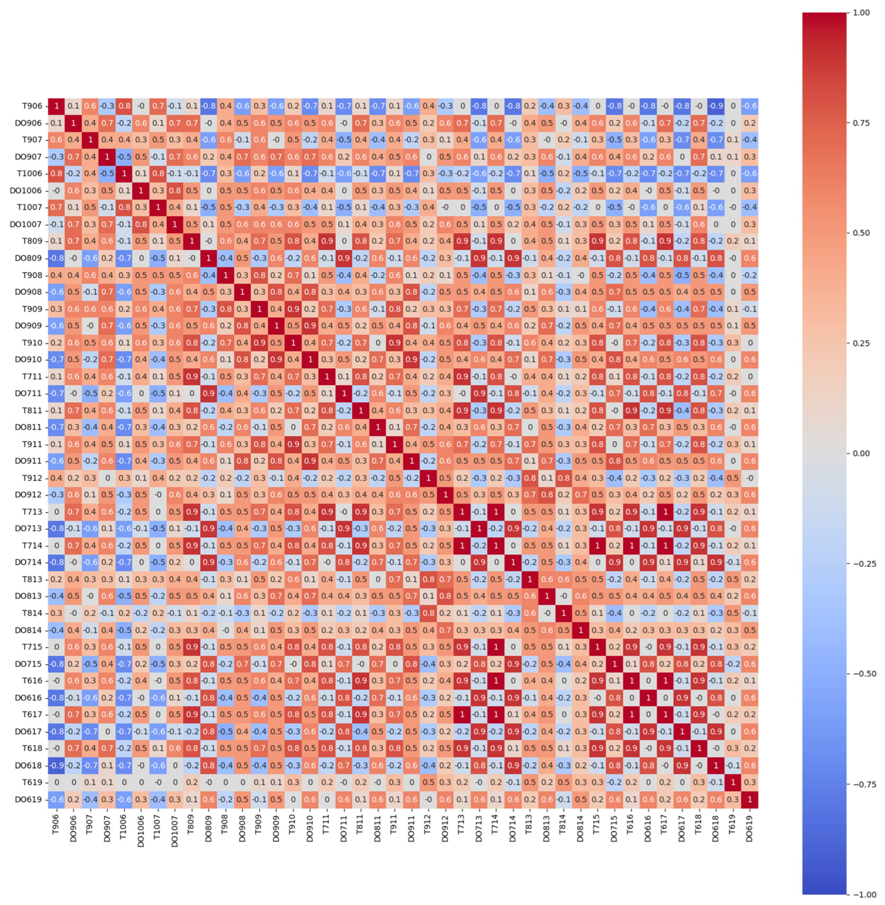
In addition, the analysis includes correlation coefficients and a heatmap depicting the relationships among all features and attributes (Figure 2). The variables are the temperature and DO concentration measured by the 21 sites shown in Table 1. The color spectrum in the heatmap reveals the strength of relationships, where a radiant red (with number 1) indicates a robust positive correlation, and a deep blue color signifies a strong negative correlation. Notably, the visual representation illustrates that temperature and DO concentration exhibit correlations with the attributes of neighboring sites, suggesting a mutual influence among these variables. Correlation indicates that the temperature and DO trends in a specific site can be inferred based on the surrounding site information because of the water flows.

2.2. Method Selection

LSTM and GRU stand out as advanced techniques in deep learning for forecasting. Evolving from the foundations of RNN, this sophisticated approach has garnered extensive attention from the research community. Over time, LSTM and GRU techniques witnessed refinements and diversifications. Various branches emerged, including convolutional LSTM, CNN-LSTM, and CNN-GRU, extending the applicability of LSTM-based and GRU-based methods.
In forecasting dissolved oxygen levels, this paper chooses LSTM and GRU, and their variants, for their proven effectiveness in modeling time-series data and handling long-term dependencies. This is crucial given the persistence of temporal patterns in water quality data. Additionally, this paper includes ConvLSTM, CNN-LSTM, and CNN-GRU, recognizing the spatial–temporal nature of the dissolved oxygen prediction task. These models, integrating convolutional and recurrent structures, excel in tasks where both spatial and temporal relationships are pivotal. The model selection meticulously aligns with the unique characteristics of the dissolved oxygen prediction task, contributing to the precision of the study outcomes.

2.2.1. LSTM-Based Methods

To mitigate the impact of extra inputs and prioritize essential ones, researchers have undertaken advancements in RNN models. A notable outcome of this effort is developing a novel model known as the LSTM model. While the LSTM model shares the fundamental principles of RNN models, it distinguishes itself through innovative mechanisms designed to enhance input selection and memory retention. The LSTM model can be described as follows:
i t = σ W i x t + W H i H t 1 + b i
f t = σ W f x t + W H f H t 1 + b f
C t ~ = tan h W C ~ x t + W H C ~ H t 1 + b C ~
o t = σ W o x t + W H o H t 1 + b o
C t = f t C t 1 + i t C t ~
H t = o t tan h C t
where i t is the input gate; f t is the forget gate; and o t   is the output gate [58,63,64,65]. The three gates are used to obtain the hidden state H t and H t 1 , and the cell state C t , C t 1 at time step t . σ denotes the sigmoid activation function; C t ~ is the candidate state; and W and b are the weight matrix and bias, respectively. denotes the Hadamard product.
The fundamental role of the forget gate is to selectively determine which information should be retained and which should be discarded within the LSTM model. This distinction is a central divergence between the LSTM and conventional RNN models. The unique quality of the LSTM model is that it efficiently retains the most important data in a predetermined amount of time. Instead of the product of weight and input, the cell state and hidden state add a new concept gate to calculate the cell and hidden gate.
The ConvLSTM and CNN-LSTM models represent specific instances of LSTM models that integrate the CNN architecture. CNNs are designed to simplify complex problem-solving tasks by emphasizing the characterization of key features within a given sample. A core aspect of a CNN’s operation is dimension reduction, aimed at condensing the essential attributes of the input object. The CNN model simplifies intricate data by employing convolution and pooling techniques.
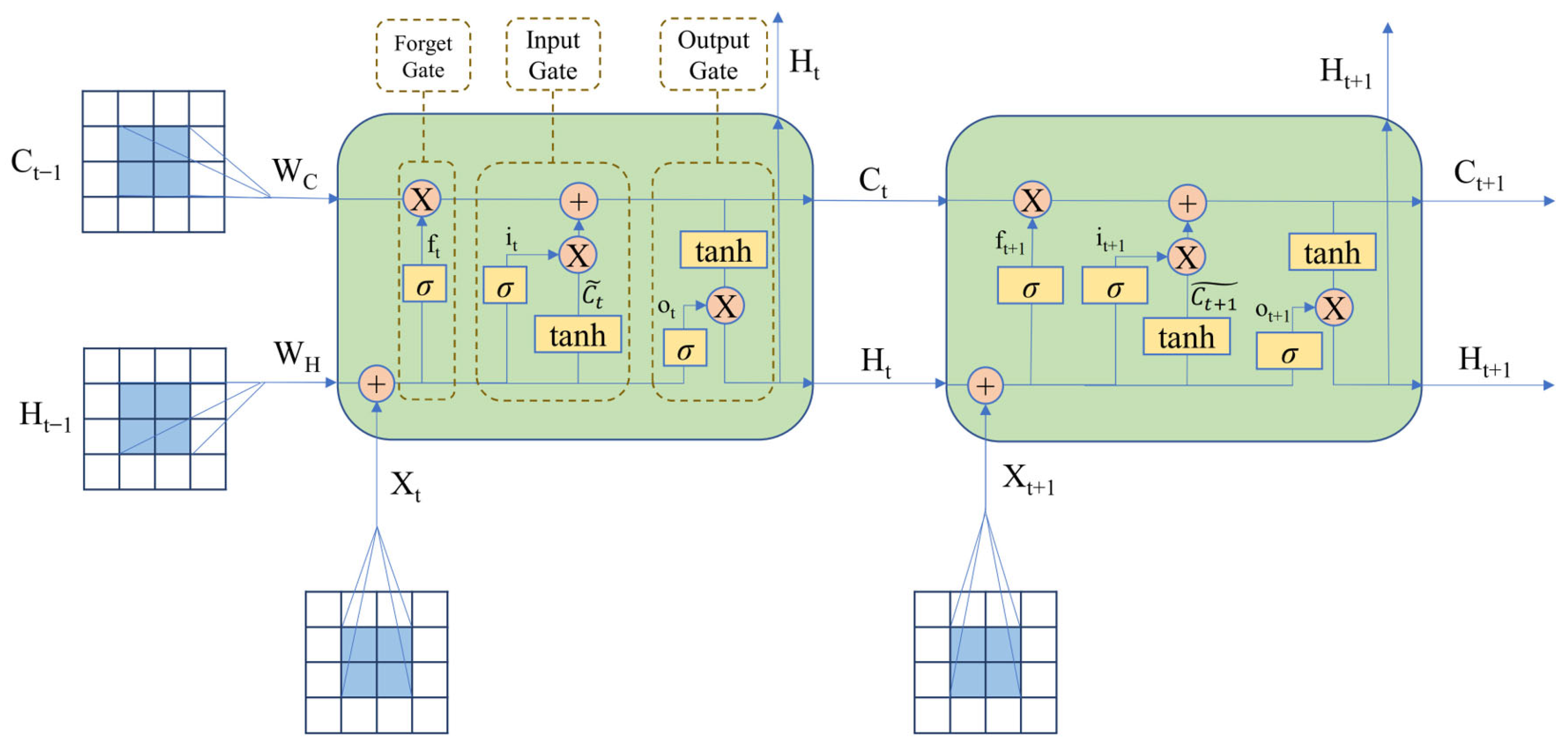
ConvLSTM and CNN-LSTM models, which are intended to analyze data with increased efficiency and efficacy, were developed due to the ability to combine CNN models with LSTM models. However, ConvLSTM and CNN-LSTM models follow distinct procedures. ConvLSTM (Figure 3) primarily employs convolutional layers to enhance the LSTM model’s performance [65], whereas the CNN-LSTM model integrates the LSTM framework to address tasks handled by the CNN model [66,67].
The LSTM, ConvLSTM, and CNN-LSTM models are renowned for their efficacy in handling complex and voluminous datasets. Ridge norm regularization and adaptive learning rate have been incorporated into the models to optimize their performance further. Ridge norm regularization limits the sizes of weights assigned to different features in the model. This is achieved by punishing large weight values. As a result, ridge regularization pushes the model to focus more on the important features, which promotes generalization. The adaptive learning rate dynamically adjusts the learning rate based on the gradients of the loss function. A large learning rate can lead to underfitting, while a small learning rate prolongs training time. Adaptive learning rates overcome these challenges by automatically adjusting the step size, thereby reducing the training time. Both ridge norm regulation and adaptive learning rate make the models robust.

2.2.2. GRU-Based Methods

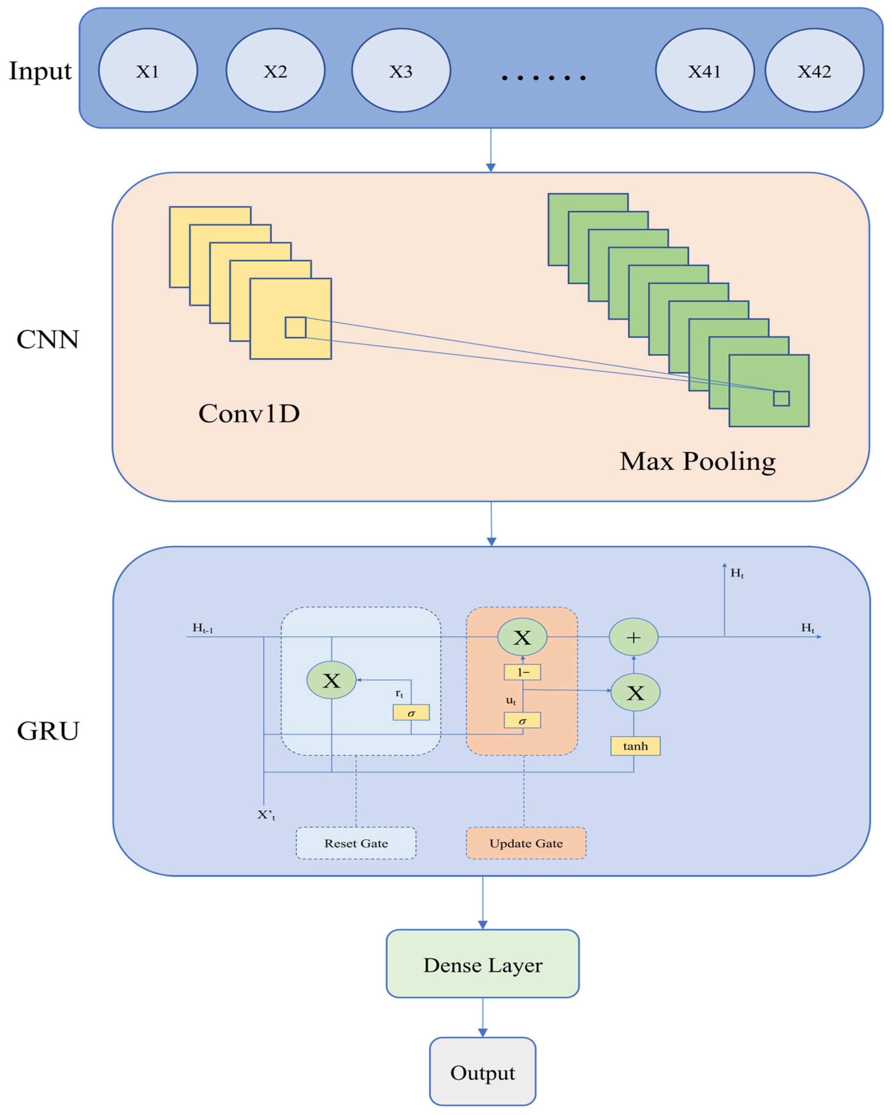
The GRU, pioneered by Cho et al. in 2014, marks a pivotal development in deep learning, particularly in RNNs. Specifically engineered to overcome the long-term dependence issues that conventional RNNs encounter, GRUs improve information flow across their design, leading to increased performance on a range of sequence data applications. GRUs are characterized by two crucial components: the update and reset gates. These gates play a crucial role in controlling the transmission of information between units; the update gate determines how much information from the previous state is carried over to the current state, while the reset gate determines how much information of the prior state should be discarded. CNNs and GRUs are combined in the CNN-GRU paradigm. CNN-GRU (Figure 4) effectively leverages the strengths of both architectures for processing sequential data that also requires the extraction of spatial features. The equations for the CNN and GRU components in such a hybrid model can be described as:
F c o n v 1 D = ReLu W c o n v 1 D x t + b c o n v 1 D
M P = MaxPooling F c o n v 1 D
r t = σ W r x t + U r H t 1 + b r
z t = σ W z x t + U z H t 1 + b z
H t ^ = tan h W H x t + U H r t H t 1 + b H
H t = z t H t 1 + 1 z t H t ^
where F c o n v 1 D is the convolution layer; ReLu is the activation function; the max pooling is used to reduce dimensionality and extract dominant features (8); r t , z t , H t ^ , and H t are the reset gate (9), the update gate (10), the candidate hidden state (11), and the final hidden state (12) vector at t ; W r , W z , W H , and W c o n v 1 D are the weight matrix for the reset gate, the update gate, the candidate hidden state, and the convolutional layers; H t 1 is the hidden state from the previous time step; x t is the current input; and b r , b z , b H , and b c o n v 1 D are the bias for the reset gate, the update gate, the candidate hidden state, and the convolutional layers. The update gate z t determines how much of the past information (from H t 1 ) to keep versus how much new information (from H t ^ ) to add.
The architecture of the GRU presents a more streamlined alternative to LSTM units, primarily by merging the forget and input gates, leading to increased efficiency in certain scenarios, especially with smaller datasets. Regarding efficiency and performance, GRUs are particularly adept at handling short-sequence data and often exhibit faster training times than LSTMs, which is attributed to their less complex structure.

2.3. Evaluation Criteria

Three primary parameters are employed in this article to assess the model’s performance: mean absolute error, root mean square error, and mean square error. These metrics also elucidate the relationships among the actual results Y i ; predicted outcomes Y i ^ ; and the mean of the actual values Y ¯ i , where n is the number of samples.
  • The mean square error (MSE)
    M S E = 1 n i = 1 n Y i Y i ^ 2
    illustrates the mean of the square of the actual results and the predicted outcome. There is an amount of data. It is a widely used parameter to determine the performance of the models. As a mathematical explanation, the MSE can also be regarded as the sum of the variance and the bias square of the predicted outcomes.
  • The mean absolute error (MAE)
    M A E = 1 n i = 1 n Y i Y i ^
    is the absolute value mean of real data and estimators. Therefore, decreasing MAE is a sign of the model improving.
  • The R-squared ( R 2 ) shows the discrepancy between the expected and actual values. The equation is given by:
    R 2 = 1 i = 1 n Y i Y i ^ 2 i = 1 n Y i Y ¯ i 2
    and is used for regression prediction. The R 2 is between 1 and 0. If the R 2 is close to 1, the regression prediction performs well.

2.4. Researching Process

This paper builds five models to determine the DO concentration in water for 1 h to 12 h ahead. All models utilized data from the year 2020 for both training and validation. Specifically, 80% of the 2020 data constituted the training dataset, while the remaining 20% served as the validation dataset. Data in 2021 were regarded as testing data. Training, validation, and testing data had a batch size of 35 and epochs of 50. The inputs were each site’s date, time, temperature, and DO concentration. The outputs were the DO concentration for 21 sites. The research involved several steps, including data collecting, data processing, model building, training and testing, performance determination, and obtaining output.

3. Results and Discussion

This study presents the development of five robust forecasting models: the LSTM, the ConvLSTM, the CNN-LSTM, the GRU, and the CNN-GRU models. Recent studies [28,68,69,70] have presented strong proof of these models’ excellence and sophistication within the water field forecasting domain. Applying these models to forecast the DO content in Lake Erie is a substantial and valuable research pursuit.

3.1. The Overturning in Lake Erie

After these models were built and the parameters were carefully adjusted, the three models that use temperature and temporal sequencing to predict hourly DO concentrations were evaluated for performance. For illustrative purposes, the results for site 714 are presented as a representative example of the modeling process.
As established in the preceding chapter, site 714 occupies a central position within Lake Erie, notably distant from the lake shore. The data acquired from this site conspicuously showcase distinctive dataset patterns. Figure 5 is a graphic depiction of the distribution of datasets for site 714 in 2020 and 2021. Notably, this figure reveals a consistent trend where DO concentration decreases with rising temperatures, a pattern observed from 19 June to 21 September in both years.
However, it is essential to highlight a significant deviation in both 2020 and 2021, marked by a sharp increase. This anomaly is attributed to a seasonal phenomenon known as overturning, a recurrent event typically occurring in autumn [21]. Overturning introduces challenges in researching temperature and other water parameters at the lakebed of Lake Erie. This, in turn, affects the accuracy of the models’ performance by compromising the integrity of dataset inputs.

3.2. Number of Hypoxia Days in the Lake Erie Central Basin

Hypoxia, a crucial environmental concern, is characterized by low oxygen levels (less than 2 mg/L) in water bodies [1,6,71,72,73,74,75]. In the initial step towards addressing this issue, this paper calculated the DO concentration for all sites and examined the frequency of hypoxic events. For Lake Erie data forecasting, hypoxia happens between the middle of July and the end of September. Table 2 presents the number of average hypoxia days for the top 11 sites in 2020 and 2021.
As evident from the table above, the occurrence of hypoxia in Lake Erie is discernible. To gain further insights into this phenomenon, the sites were categorized into two distinct groups: those situated near the lakeshore and those positioned farther away. Remarkably, the sites far from the lake shore often confront hypoxia due to their proximity to urban areas, such as the site near Cleveland. These urban areas are associated with elevated pollution emissions, significantly contributing to hypoxia [5,76,77,78].

3.3. The Performance of Machine Learning Models

After constructing these models and meticulously fine-tuning their parameters, we conducted predictive experiments employing a batch size of 35 and an epoch count of 50. These experiments were designed to forecast DO concentration across time intervals spanning from 1 to 12 h. Following these predictions, we assessed the model’s performance by computing the key performance metrics, which include MSE, MAE, and R-square ( R 2 ). Table 3 introduces the training and testing performance metrics 1, 3, 6, and 12 h ahead, specifically MSE, MAE, and R 2 , applied to the forecasting of DO concentration using the dataset from site 714.
As indicated in Table 3, the performance metrics for all five models during the training process demonstrate commendable results. The MSE and MAE exhibit low values, while the R 2 coefficient approaches unity. These outcomes collectively suggest robust and effective performance across various measurement indicators. Based on Table 3, three LSTM-based and two GRU-based models accurately forecasted the DO concentration from 1 to 12 h. The ConvLSTM and CNN-GRU models outperformed all other models.
After evaluating the forecasted and actual values for both the 1 h and 12 h predictions (Figure 6), we found that the predicted values exhibit a similar pattern to the actual values. Despite this congruence, differences persist between the forecasted and actual values. This variance can be attributed to dataset limitations, which lack extensive time sequence information and fail to capture the periodic overturning phenomenon observed in Lake Erie. Achieving a more accurate result necessitates a dataset with more detailed features and a comprehensive representation of temporal dynamics.
There are still many other methods used for dissolved oxygen forecasting. Table 4 introduces some of the latest methods in dissolved oxygen prediction.
Based on the findings presented in Table 4, the ConvLSTM model, which exhibits the best performance in this study, demonstrates good outcomes when compared to the four latest methods evaluated. The ConvLSTM model has a high R 2 and low MSE and MAE. As also shown in this table, advancements in science have led to the widespread adoption of deep learning and neural network models such as ConvLSTM, LSTM, CNN-LSTM, K-medoids-LRELM, and BBO-ANN due to their enhanced performance capabilities [49,53,54,79,80]. However, these models encounter persistent challenges despite their efficacy, particularly when confronted with small datasets lacking regularity. Overfitting and underfitting pose significant threats to model robustness in such scenarios. Remarkably, the ConvLSTM model implemented in this study successfully forecasts dissolved oxygen levels in Lake Erie, a dataset characterized by its limited size and inherent variability. Despite these challenges, our models exhibit commendable robustness, underscoring their efficacy in real-world applications.

3.4. The Features’ Contribution to DO Prediction

While conducting hypoxia research in Lake Erie, site 811 emerged as a site of paramount significance. However, the identification of other pivotal sites is equally imperative. To ascertain their relative importance, the Shapley additive explanations (SHAP) model is employed, offering valuable insights into the contributions of each feature when used for prediction. In essence, the SHAP model provides a measure of feature importance, aiding in delineating key sites for further research and investigation.
Figure 7a presents a SHAP plot delineating the individual contributions of various features when forecasting DO concentrations for site 811. The previous analysis has established the central positioning of site 811 within the hypoxia-affected region. To determine additional sites of significance for hypoxia research, site 811 can serve as a reference point.
Referencing Figure 7b, the SHAP graph specific to site 714 is presented. Site 714, as previously discussed, holds significance in our analysis. The temperature observed at site 713 continues to be a significant contributing element in the prediction of the DO content at site 714, according to an examination of the SHAP graph. Notably, this contribution is evident not only in terms of positive impact but also negatively influences the predicted outcome.
Figure 7 notably highlights the top 21 influential features, encompassing temperature and DO measurements from 21 distinct sites. Among these, the temperature recorded at site 713 emerges as the most pivotal feature with the most substantial influence on DO concentration forecasting. A rise in temperature at site 713 corresponds to a positive impact on the model’s output. Additionally, DO concentration and temperature readings from sites 912 and 811 are also noteworthy features, contributing to changes in forecasting results. Conversely, the remaining features exert relatively less influence on the predicted DO concentration changes.

4. Conclusions

DO serves as the primary water quality indicator for assessing the health of freshwater lake ecosystems. Low DO levels cause the death of aquatic life. Lake Erie, supporting numerous aquatic organisms and over 11 million people, experiences deficient DO levels (hypoxia) in the central basin from mid-July through September. Consequently, extensive research efforts by both government agencies and academia have been dedicated to understanding DO fluctuations in Lake Erie. Forecasting DO proves instrumental for environmental protection agencies, enabling them to anticipate and evaluate ecological impacts, and implement effective management policies.
To address the crucial need for accurate DO concentration forecasts, this study employs advanced models, including LSTM, CNN-LSTM, ConvLSTM, GRU, and CNN-GRU. The integration of these hybrid algorithms enhances spatio-temporal time-series predictions, particularly for capturing spatially complex 3D and nonlinear dynamic DO concentration fluctuations in the expansive lake environment. ConvLSTM, incorporating convolution operations within the LSTM cell, enhances spatial feature capture. Integration of CNN with LSTM and GRU allows for effective data processing and subsequent handling of one-dimensional temporal variations in the resulting feed.
In this paper, the dataset used for training and testing features temperature and DO concentration for 21 sites. After analyzing the input features, the output is the predicted DO concentration. Model performance evaluation, employing metrics such as MSE, MAE, and R 2 , reveals that ConvLSTM outperforms other models for forecasting dissolved oxygen concentrations up to 12 h ahead.
Additionally, SHAP models were applied to analyze key factors’ importance, such as water temperature and DO concentration in adjacent stations, for forecasting DO concentrations at the target site. The temperature in site 713 emerges as crucial information for DO concentrations in Lake Erie’s Central Basin.
In conclusion, this research significantly advances DO prediction methodologies in Lake Erie, demonstrating the efficacy of hybrid models and shedding light on critical factors influencing accurate forecasts. The outcomes contribute to informed decision-making for environmental protection and resource management, fostering a comprehensive understanding of the dynamic interactions within the lake ecosystem.

Author Contributions

Conceptualization: D.P.; methodology: D.P. and Y.Z.; software: D.P. and Y.Z.; validation: D.P.; formal analysis: D.P.; investigation: D.P.; resources: D.P., Y.D. and B.G.; data curation: D.P.; writing—original draft preparation: D.P., Y.Z., Y.D., B.G., J.V.G.T. and S.X.Y.; writing—review and editing: B.G., J.V.G.T. and S.X.Y.; supervision: B.G. and S.X.Y.; project administration: B.G., S.X.Y. and J.V.G.T.; funding acquisition: B.G. All authors have read and agreed to the published version of the manuscript.

Funding

This research was funded by the Natural Sciences and Engineering Research Council of Canada (NSERC) Alliance Grant #401643.

Data Availability Statement

Data are contained within the article.

Conflicts of Interest

Author Jesse Van Griensven is employed by the company Lakes Software. The remaining authors declare that the research was conducted in the absence of any commercial or financial relationships that could be construed as a potential conflict of interest.

References

  1. Gorgan-Mohammadi, F.; Rajaee, T.; Zounemat-Kermani, M. Decision tree models in predicting water quality parameters of dissolved oxygen and phosphorus in lake water. Sustain. Water Resour. Manag. 2023, 9, 1. [Google Scholar] [CrossRef]
  2. McLaren, J.S.; Van Kirk, R.W.; Mabaka, A.J.; Brothers, S.; Budy, P. Drawdown, Habitat, and Kokanee Populations in a Western US Reservoir. N. Am. J. Fish. Manag. 2023, 43, 339–351. [Google Scholar] [CrossRef]
  3. Kumar, S.; Dubey, M.; Kumar, A. Metabolic Adaptation of Fishes Under Different Consequences of Climate Change. In Outlook of Climate Change and Fish Nutrition; Springer: Singapore, 2023; pp. 121–132. [Google Scholar]
  4. Cavole, L.M.; Limburg, K.E.; Gallo, N.D.; Salvanes, A.G.V.; Ramírez-Valdez, A.; Levin, L.A.; Oropeza, O.A.; Hertwig, A.; Liu, M.C.; McKeegan, K.D. Otoliths of marine fishes record evidence of low oxygen, temperature and pH conditions of deep Oxygen Minimum Zones. Deep Sea Res. Part I Oceanogr. Res. Pap. 2023, 191, 103941. [Google Scholar] [CrossRef]
  5. Watson, S.B.; Miller, C.; Arhonditsis, G.; Boyer, G.L.; Carmichael, W.; Charlton, M.N.; Confesor, R.; Depew, D.C.; Höök, T.O.; Ludsin, S.A.; et al. The re-eutrophication of Lake Erie: Harmful algal blooms and hypoxia. Harmful Algae 2016, 56, 44–66. [Google Scholar] [CrossRef]
  6. Scavia, D.; Allan, J.D.; Arend, K.K.; Bartell, S.; Beletsky, D.; Bosch, N.S.; Brandt, S.B.; Briland, R.D.; Daloğlu, I.; DePinto, J.V.; et al. Assessing and addressing the re-eutrophication of Lake Erie: Central basin hypoxia. J. Great Lakes Res. 2014, 40, 226–246. [Google Scholar] [CrossRef]
  7. Jane, S.F.; Hansen, G.J.; Kraemer, B.M.; Leavitt, P.R.; Mincer, J.L.; North, R.L.; Pilla, R.M.; Stetler, J.T.; Williamson, C.E.; Woolway, R.I.; et al. Widespread deoxygenation of temperate lakes. Nature 2021, 594, 66–70. [Google Scholar] [CrossRef]
  8. Global Great Lakes. Lake Erie Overview. Available online: https://globalgreatlakes.org/lgl/erie/index.html (accessed on 30 December 2023).
  9. Karatayev, A.Y.; Burlakova, L.E.; Hrycik, A.R.; Daniel, S.E.; Mehler, K.; Hinchey, E.K.; Dermott, R.; Griffiths, R. Long-term dynamics of Lake Erie benthos: One lake, three distinct communities. J. Great Lakes Res. 2022, 48, 1599–1617. [Google Scholar] [CrossRef]
  10. Wu, N.; Huang, J.; Schmalz, B.; Fohrer, N. Modeling daily chlorophyll a dynamics in a German lowland river using artificial neural networks and multiple linear regression approaches. Limnology 2014, 15, 47–56. [Google Scholar] [CrossRef]
  11. Seo, Y.; Kim, S.; Kisi, O.; Singh, V.P. Daily water level forecasting using wavelet decomposition and artificial intelligence techniques. J. Hydrol. 2015, 520, 224–243. [Google Scholar] [CrossRef]
  12. Ji, X.; Shang, X.; Dahlgren, R.A.; Zhang, M. Prediction of dissolved oxygen concentration in hypoxic river systems using support vector machine: A case study of Wen-Rui Tang River, China. Environ. Sci. Pollut. Res. 2017, 24, 16062–16076. [Google Scholar] [CrossRef]
  13. Olyaie, E.; Abyaneh, H.Z.; Mehr, A.D. A comparative analysis among computational intelligence techniques for dissolved oxygen prediction in Delaware River. Geosci. Front. 2017, 8, 517–527. [Google Scholar] [CrossRef]
  14. Heddam, S.; Kisi, O. Modelling daily dissolved oxygen concentration using least square support vector machine, multivariate adaptive regression splines and M5 model tree. J. Hydrol. 2018, 559, 499–509. [Google Scholar] [CrossRef]
  15. Kim, H.G.; Hong, S.; Jeong, K.S.; Kim, D.K.; Joo, G.J. Determination of sensitive variables regardless of hydrological alteration in artificial neural network model of chlorophyll a: Case study of Nakdong River. Ecol. Model. 2019, 398, 67–76. [Google Scholar] [CrossRef]
  16. Ahmed, M.H.; Lin, L.S. Dissolved oxygen concentration predictions for running waters with different land use land cover using a quantile regression forest machine learning technique. J. Hydrol. 2021, 597, 126213. [Google Scholar] [CrossRef]
  17. Ranković, V.; Radulović, J.; Radojević, I.; Ostojić, A.; Čomić, L. Neural network modeling of dissolved oxygen in the Gruža reservoir, Serbia. Ecol. Model. 2010, 221, 1239–1244. [Google Scholar] [CrossRef]
  18. Ay, M.; Kisi, O. Modeling of dissolved oxygen concentration using different neural network techniques in Foundation Creek, El Paso County, Colorado. J. Environ. Eng. 2012, 138, 654–662. [Google Scholar] [CrossRef]
  19. Antanasijević, D.; Pocajt, V.; Perić-Grujić, A.; Ristić, M. Modelling of dissolved oxygen in the Danube River using artificial neural networks and Monte Carlo Simulation uncertainty analysis. J. Hydrol. 2014, 519, 1895–1907. [Google Scholar] [CrossRef]
  20. Li, W.; Wu, H.; Zhu, N.; Jiang, Y.; Tan, J.; Guo, Y. Prediction of dissolved oxygen in a fishery pond based on gated recurrent unit (GRU). Inf. Process. Agric. 2021, 8, 185–193. [Google Scholar] [CrossRef]
  21. Li, W.; Fang, H.; Qin, G.; Tan, X.; Huang, Z.; Zeng, F.; Du, H.; Li, S. Concentration estimation of dissolved oxygen in Pearl River Basin using input variable selection and machine learning techniques. Sci. Total Environ. 2020, 731, 139099. [Google Scholar] [CrossRef]
  22. Zhu, S.; Heddam, S. Prediction of dissolved oxygen in urban rivers at the Three Gorges Reservoir, China: Extreme learning machines (ELM) versus artificial neural network (ANN). Water Qual. Res. J. 2020, 55, 106–118. [Google Scholar] [CrossRef]
  23. Cao, X.; Ren, N.; Tian, G.; Fan, Y.; Duan, Q. A three-dimensional prediction method of dissolved oxygen in pond culture based on Attention-GRU-GBRT. Comput. Electron. Agric. 2021, 181, 105955. [Google Scholar] [CrossRef]
  24. Wang, Z.; Wang, Q.; Liu, Z.; Wu, T. A deep learning interpretable model for river dissolved oxygen multi-step and interval prediction based on multi-source data fusion. J. Hydrol. 2024, 629, 130637. [Google Scholar] [CrossRef]
  25. Hochreiter, S.; Schmidhuber, J. Long short-term memory. Neural Comput. 1997, 9, 1735–1780. [Google Scholar] [CrossRef]
  26. Jordan, M.I. Serial order: A parallel distributed processing approach. In Advances in Psychology; Elsevier: Amsterdam, The Netherlands, 1997; Volume 121, pp. 471–495. [Google Scholar]
  27. Xue, P.; Wagh, A.; Ma, G.; Wang, Y.; Yang, Y.; Liu, T.; Huang, C. Integrating Deep Learning and Hydrodynamic Modeling to Improve the Great Lakes Forecast. Remote Sens. 2022, 14, 2640. [Google Scholar] [CrossRef]
  28. Liu, W.; Wang, Y.; Zhong, D.; Xie, S.; Xu, J. ConvLSTM Network-Based Rainfall Nowcasting Method with Combined Reflectance and Radar-Retrieved Wind Field as Inputs. Atmosphere 2022, 13, 411. [Google Scholar] [CrossRef]
  29. Huang, R.; Ma, C.; Ma, J.; Huangfu, X.; He, Q. Machine learning in natural and engineered water systems. Water Res. 2021, 205, 117666. [Google Scholar] [CrossRef]
  30. Zheng, L.; Wang, H.; Liu, C.; Zhang, S.; Ding, A.; Xie, E.; Li, J.; Wang, S. Prediction of harmful algal blooms in large water bodies using the combined EFDC and LSTM models. J. Environ. Manag. 2021, 295, 113060. [Google Scholar] [CrossRef]
  31. Liang, Z.; Zou, R.; Chen, X.; Ren, T.; Su, H.; Liu, Y. Simulate the forecast capacity of a complicated water quality model using the long short-term memory approach. J. Hydrol. 2020, 581, 124432. [Google Scholar] [CrossRef]
  32. Hu, Z.; Zhang, Y.; Zhao, Y.; Xie, M.; Zhong, J.; Tu, Z.; Liu, J. A water quality prediction method based on the deep LSTM network considering correlation in smart mariculture. Sensors 2019, 19, 1420. [Google Scholar] [CrossRef] [PubMed]
  33. Pyo, J.; Pachepsky, Y.; Kim, S.; Abbas, A.; Kim, M.; Kwon, Y.S.; Ligaray, M.; Cho, K.H. Long short-term memory models of water quality in inland water environments. Water Res. X 2023, 21, 100207. [Google Scholar] [CrossRef] [PubMed]
  34. Liu, P.; Wang, J.; Sangaiah, A.K.; Xie, Y.; Yin, X. Analysis and prediction of water quality using LSTM deep neural networks in IoT environment. Sustainability 2019, 11, 2058. [Google Scholar] [CrossRef]
  35. Kim, Y.W.; Kim, T.; Shin, J.; Go, B.; Lee, M.; Lee, J.; Koo, J.; Cho, K.H.; Cha, Y. Forecasting abrupt depletion of dissolved oxygen in urban streams using discontinuously measured hourly time-series data. Water Resour. Res. 2021, 57, e2020WR029188. [Google Scholar] [CrossRef]
  36. Cao, X.; Liu, Y.; Wang, J.; Liu, C.; Duan, Q. Prediction of dissolved oxygen in pond culture water based on K-means clustering and gated recurrent unit neural network. Aquac. Eng. 2020, 91, 102122. [Google Scholar] [CrossRef]
  37. Abba, S.I.; Linh, N.T.T.; Abdullahi, J.; Ali, S.I.A.; Pham, Q.B.; Abdulkadir, R.A.; Costache, R.; Anh, D.T. Hybrid machine learning ensemble techniques for modeling dissolved oxygen concentration. IEEE Access 2020, 8, 157218–157237. [Google Scholar] [CrossRef]
  38. Nanyang, Z.; Hao, W.; Daheng, Y.; Zhiqiang, W.; Yongnian, J.; Ya, G. An improved method for estimating dissolved oxygen in crab ponds based on Long Short-Term Memory. Smart Agric. 2019, 1, 67. [Google Scholar]
  39. Zhu, N.; Ji, X.; Tan, J.; Jiang, Y.; Guo, Y. Prediction of dissolved oxygen concentration in aquatic systems based on transfer learning. Comput. Electron. Agric. 2021, 180, 105888. [Google Scholar] [CrossRef]
  40. Wai, K.P.; Chia, M.Y.; Koo, C.H.; Huang, Y.F.; Chong, W.C. Applications of deep learning in water quality management: A state-of-the-art review. J. Hydrol. 2022, 613, 128332. [Google Scholar] [CrossRef]
  41. LeCun, Y.; Boser, B.; Denker, J.S.; Henderson, D.; Howard, R.E.; Hubbard, W.; Jackel, L.D. Backpropagation applied to handwritten zip code recognition. Neural Comput. 1989, 1, 541–551. [Google Scholar] [CrossRef]
  42. Khosravi, K.; Panahi, M.; Golkarian, A.; Keesstra, S.D.; Saco, P.M.; Bui, D.T.; Lee, S. Convolutional neural network approach for spatial prediction of flood hazard at national scale of Iran. J. Hydrol. 2020, 591, 125552. [Google Scholar] [CrossRef]
  43. Chen, H.; Chen, A.; Xu, L.; Xie, H.; Qiao, H.; Lin, Q.; Cai, K. A deep learning CNN architecture applied in smart near-infrared analysis of water pollution for agricultural irrigation resources. Agric. Water Manag. 2020, 240, 106303. [Google Scholar] [CrossRef]
  44. Yan, J.; Liu, J.; Yu, Y.; Xu, H. Water quality prediction in the luan river based on 1-drcnn and bigru hybrid neural network model. Water 2021, 13, 1273. [Google Scholar] [CrossRef]
  45. Barzegar, R.; Aalami, M.T.; Adamowski, J. Short-term water quality variable prediction using a hybrid CNN–LSTM deep learning model. Stoch. Environ. Res. Risk Assess. 2020, 34, 415–433. [Google Scholar] [CrossRef]
  46. Barzegar, R.; Aalami, M.T.; Adamowski, J. Coupling a hybrid CNN-LSTM deep learning model with a boundary corrected maximal overlap discrete wavelet transform for multiscale lake water level forecasting. J. Hydrol. 2021, 598, 126196. [Google Scholar] [CrossRef]
  47. Baek, S.S.; Pyo, J.; Chun, J.A. Prediction of water level and water quality using a CNN-LSTM combined deep learning approach. Water 2020, 12, 3399. [Google Scholar] [CrossRef]
  48. Yang, Y.; Xiong, Q.; Wu, C.; Zou, Q.; Yu, Y.; Yi, H.; Gao, M. A study on water quality prediction by a hybrid CNN-LSTM model with attention mechanism. Environ. Sci. Pollut. Res. 2021, 28, 55129–55139. [Google Scholar] [CrossRef]
  49. Hu, Y.; Liu, C.; Wollheim, W.M. Prediction of riverine daily minimum dissolved oxygen concentrations using hybrid deep learning and routine hydrometeorological data. Sci. Total Environ. 2024, 918, 170383. [Google Scholar] [CrossRef]
  50. Yang, J. Predicting water quality through daily concentration of dissolved oxygen using improved artificial intelligence. Sci. Rep. 2023, 13, 20370. [Google Scholar] [CrossRef]
  51. Shi, X.; Chen, Z.; Wang, H.; Yeung, D.Y.; Wong, W.K.; Woo, W.c. Convolutional LSTM network: A machine learning approach for precipitation nowcasting. Adv. Neural Inf. Process. Syst. 2015, 28, 802–810. [Google Scholar]
  52. Moghadam, S.V.; Sharafati, A.; Feizi, H.; Marjaie, S.M.S.; Asadollah, S.B.H.S.; Motta, D. An efficient strategy for predicting river dissolved oxygen concentration: Application of deep recurrent neural network model. Environ. Monit. Assess. 2021, 193, 798. [Google Scholar] [CrossRef] [PubMed]
  53. Azma, A.; Liu, Y.; Azma, M.; Saadat, M.; Zhang, D.; Cho, J.; Rezania, S. Hybrid machine learning models for prediction of daily dissolved oxygen. J. Water Process Eng. 2023, 54, 103957. [Google Scholar] [CrossRef]
  54. Ayesha Jasmin, S.; Ramesh, P.; Tanveer, M. An intelligent framework for prediction and forecasting of dissolved oxygen level and biofloc amount in a shrimp culture system using machine learning techniques. Expert Syst. Appl. 2022, 199, 117160. [Google Scholar] [CrossRef]
  55. Bolick, M.M.; Post, C.J.; Naser, M.Z.; Mikhailova, E.A. Comparison of machine learning algorithms to predict dissolved oxygen in an urban stream. Environ. Sci. Pollut. Res. 2023, 30, 78075–78096. [Google Scholar] [CrossRef]
  56. Roushangar, K.; Davoudi, S.; Shahnazi, S. The potential of novel hybrid SBO-based long short-term memory network for prediction of dissolved oxygen concentration in successive points of the Savannah River, USA. Environ. Sci. Pollut. Res. 2023, 30, 46960–46978. [Google Scholar] [CrossRef] [PubMed]
  57. Ali, M.; Khan, D.M.; Alshanbari, H.M.; El-Bagoury, A.A.A.H. Prediction of complex stock market data using an improved hybrid emd-lstm model. Appl. Sci. 2023, 13, 1429. [Google Scholar] [CrossRef]
  58. Zhang, Y.; Gu, Z.; Thé, J.V.G.; Yang, S.X.; Gharabaghi, B. The Discharge Forecasting of Multiple Monitoring Station for Humber River by Hybrid LSTM Models. Water 2022, 14, 1794. [Google Scholar] [CrossRef]
  59. Kuo, C.E.; Chen, G.T. Automatic sleep staging based on a hybrid stacked LSTM neural network: Verification using large-scale dataset. IEEE Access 2020, 8, 111837–111849. [Google Scholar] [CrossRef]
  60. Pilla, R.M.; Williamson, C.E.; Adamovich, B.V.; Adrian, R.; Anneville, O.; Chandra, S.; Colom-Montero, W.; Devlin, S.P.; Dix, M.A.; Dokulil, M.T.; et al. Deeper waters are changing less consistently than surface waters in a global analysis of 102 lakes. Sci. Rep. 2020, 10, 20514. [Google Scholar] [CrossRef]
  61. Kralj, M.; Lipizer, M.; Čermelj, B.; Celio, M.; Fabbro, C.; Brunetti, F.; Francé, J.; Mozetič, P.; Giani, M. Hypoxia and dissolved oxygen trends in the northeastern Adriatic Sea (Gulf of Trieste). Deep Sea Res. Part II Top. Stud. Oceanogr. 2019, 164, 74–88. [Google Scholar] [CrossRef]
  62. Oldham, R.; Kraus, R. Bottom Dissolved Oxygen Measurements from Lake Erie’s Central Basin, 2021: U.S. Geological Survey Data Release; U.S. Geological Survey: Reston, VA, USA, 2022. [CrossRef]
  63. Koutsovili, E.I.; Tzoraki, O.; Theodossiou, N.; Tsekouras, G.E. Early Flood Monitoring and Forecasting System Using a Hybrid Machine Learning-Based Approach. ISPRS Int. J. Geo-Inf. 2023, 12, 464. [Google Scholar] [CrossRef]
  64. Shahid, F.; Zameer, A.; Muneeb, M. A novel genetic LSTM model for wind power forecast. Energy 2021, 223, 120069. [Google Scholar] [CrossRef]
  65. Tabrizi, S.E.; Xiao, K.; Thé, J.V.G.; Saad, M.; Farghaly, H.; Yang, S.X.; Gharabaghi, B. Hourly road pavement surface temperature forecasting using deep learning models. J. Hydrol. 2021, 603, 126877. [Google Scholar] [CrossRef]
  66. Shi, C.; Zhang, Z.; Zhang, W.; Zhang, C.; Xu, Q. Learning Multiscale Temporal–Spatial–Spectral Features via a Multipath Convolutional LSTM Neural Network for Change Detection With Hyperspectral Images. IEEE Trans. Geosci. Remote Sens. 2022, 60, 1–16. [Google Scholar] [CrossRef]
  67. Rahman, S.A.; Adjeroh, D.A. Deep learning using convolutional LSTM estimates biological age from physical activity. Sci. Rep. 2019, 9, 11425. [Google Scholar] [CrossRef] [PubMed]
  68. Zhang, Y.; Zhou, Z.; Van Griensven Thé, J.; Yang, S.X.; Gharabaghi, B. Flood Forecasting Using Hybrid LSTM and GRU Models with Lag Time Preprocessing. Water 2023, 15, 3982. [Google Scholar] [CrossRef]
  69. Haq, K.R.A.; Harigovindan, V. Water quality prediction for smart aquaculture using hybrid deep learning models. IEEE Access 2022, 10, 60078–60098. [Google Scholar]
  70. Zhang, Y.; Pan, D.; Van Griensven, J.; Yang, S.X.; Gharabaghi, B. Intelligent flood forecasting and warning: A survey. Intell. Robot. 2023, 3, 190–212. [Google Scholar] [CrossRef]
  71. Anderson, E.J.; Stow, C.A.; Gronewold, A.D.; Mason, L.A.; McCormick, M.J.; Qian, S.S.; Ruberg, S.A.; Beadle, K.; Constant, S.A.; Hawley, N. Seasonal overturn and stratification changes drive deep-water warming in one of Earth’s largest lakes. Nat. Commun. 2021, 12, 1688. [Google Scholar] [CrossRef] [PubMed]
  72. Dugener, N.M.; Stone, I.P.; Weinke, A.D.; Biddanda, B.A. Out of oxygen: Stratification and loading drove hypoxia during a warm, wet, and productive year in a Great Lakes estuary. J. Great Lakes Res. 2023, 49, 1015–1028. [Google Scholar] [CrossRef]
  73. Jabbari, A.; Ackerman, J.D.; Boegman, L.; Zhao, Y. Episodic hypoxia in the western basin of Lake Erie. Limnol. Oceanogr. 2019, 64, 2220–2236. [Google Scholar] [CrossRef]
  74. Zhou, Y.; Obenour, D.R.; Scavia, D.; Johengen, T.H.; Michalak, A.M. Spatial and temporal trends in Lake Erie hypoxia, 1987–2007. Environ. Sci. Technol. 2013, 47, 899–905. [Google Scholar] [CrossRef]
  75. Rao, Y.R.; Hawley, N.; Charlton, M.N.; Schertzer, W.M. Physical processes and hypoxia in the central basin of Lake Erie. Limnol. Oceanogr. 2008, 53, 2007–2020. [Google Scholar] [CrossRef]
  76. Uejio, C.K.; Gonsoroski, E.; Sherchan, S.P.; Beitsch, L.; Harville, E.; Blackmore, C.; Pan, K.; Lichtveld, M.Y. Harmful algal bloom-related 311 calls, Cape Coral, Florida 2018–2019. J. Water Health 2022, 20, 531–538. [Google Scholar] [CrossRef] [PubMed]
  77. Scavia, D.; Wang, Y.C.; Obenour, D.R. Advancing freshwater ecological forecasts: Harmful algal blooms in Lake Erie. Sci. Total Environ. 2023, 856, 158959. [Google Scholar] [CrossRef] [PubMed]
  78. Xu, W.; Collingsworth, P.D.; Kraus, R.; Minsker, B. Spatio-Temporal Analysis of Hypoxia in the Central Basin of Lake Erie of North America. Water Resour. Res. 2021, 57, e2020WR027676. [Google Scholar] [CrossRef]
  79. Saeed, A.; Alsini, A.; Amin, D. Water quality multivariate forecasting using deep learning in a West Australian estuary. Environ. Model. Softw. 2024, 171, 105884. [Google Scholar] [CrossRef]
  80. Shi, P.; Kuang, L.; Yuan, L.; Wang, Q.; Li, G.; Yuan, Y.; Zhang, Y.; Huang, G. Dissolved oxygen prediction using regularized extreme learning machine with clustering mechanism in a black bass aquaculture pond. Aquac. Eng. 2024, 105, 102408. [Google Scholar] [CrossRef]
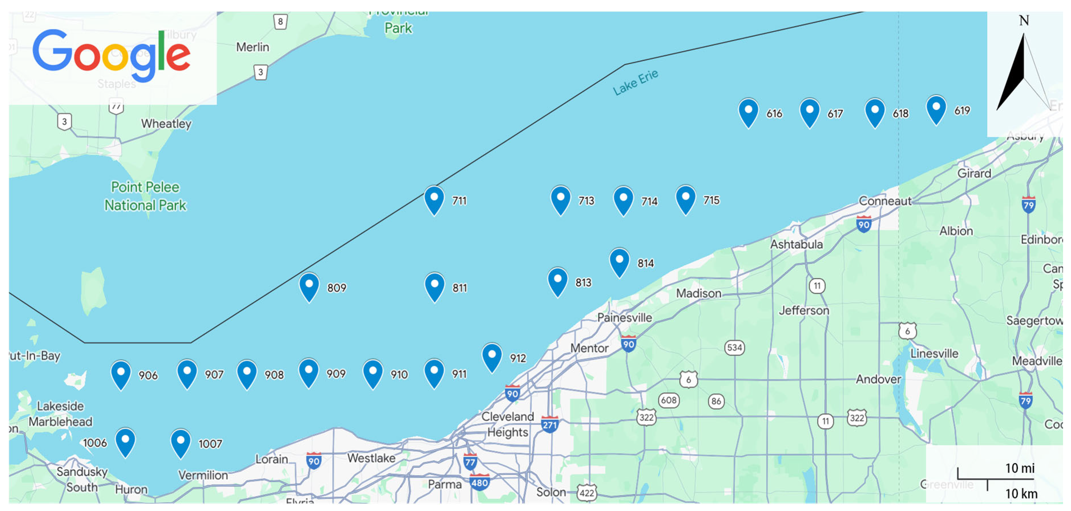
Figure 1. The location of the 21 Lake Erie Central Basin near-bottom water quality monitoring sites.
Water 16 00707 g001
Figure 2. The correlation coefficient of the features for the 21 sites.
Water 16 00707 g002
Figure 3. The architecture of ConvLSTM models.
Water 16 00707 g003
Figure 4. The architecture of CNN-GRU models.
Water 16 00707 g004
Figure 5. The observed water temperature and DO concentrations for site 714 in (a) 2020 and (b) 2021.
Water 16 00707 g005aWater 16 00707 g005b
Figure 6. The comparison between (a) 1 h and (b) 12 h ahead actual versus ConvLSTM model forecasts.
Water 16 00707 g006
Figure 7. The feature contribution plots for sites (a) 811 and (b) 714.
Water 16 00707 g007
Table 1. The geographic information of the 21 sites.
SiteLongitude (W)Latitude (N)SitesLongitude (W)Latitude (N)SitesLongitude (W)Latitude (N)
61680.917742.083671581.084641.917990882.249041.5838
61780.755942.083180982.082941.750190982.085341.5857
61880.582842.083381181.750441.750191081.915041.5839
61980.419442.089381381.424241.760691181.751741.5853
71181.751541.917181481.260041.797491281.598341.6154
71381.416241.916990682.583241.5826100682.572041.4528
71481.249641.915790782.407441.584100782.424541.4508
Table 2. The average number of hypoxia dates for the top 11 sites.
Site IDAverage Number of Hypoxia Days
91140
80931
90931
81331
90727
91027
71125
71323
90820
91220
71417
Table 3. The training and testing performance statistics of the machine learning models.
Hours AheadModelTraining
MSE
Training
MAE
Training
R 2
Testing
MSE
Testing
MAE
Testing
R 2
1LSTM0.38770.50260.95641.34680.78100.8573
1GRU0.19690.31690.97790.94770.67850.8995
1CNN-LSTM0.38560.47280.95661.51180.83380.8398
1CNN-GRU0.12870.24660.98550.83590.64320.9114
1ConvLSTM0.21190.36340.97620.28420.36220.9699
3LSTM0.33450.44120.96231.41170.79080.8503
3GRU0.19730.31830.97781.0020.68890.8938
3CNN-LSTM0.34800.45300.96081.55300.84260.8354
3CNN-GRU0.12590.24590.98580.87570.65110.9092
3ConvLSTM0.18820.34280.97880.32080.38370.9685
6LSTM0.39880.47270.95491.46440.79550.8447
6GRU0.21220.33030.97601.06560.70080.8870
6CNN-LSTM0.39060.47430.95581.58890.84540.8315
6CNN-GRU0.14160.25710.98400.94490.66230.8998
6ConvLSTM0.19840.35160.97760.38250.38990.9594
12LSTM0.52150.51570.94071.59170.83590.8310
12GRU0.26270.35950.97011.23500.73290.8689
12CNN-LSTM0.42490.50030.95171.70680.86120.8188
12CNN-GRU0.21670.29410.97541.08360.68200.8850
12ConvLSTM0.27710.38370.96850.50920.41720.9460
Table 4. Some of the latest methods used in dissolved oxygen prediction.
ModelReferencePerformance
ConvLSTMThis paper MSE = 0.5092 ,   MAE = 0.4172 ,   R 2 = 0.9460
LSTMSaeed et al. (2024) [79] R 2 = 0.910
CNN-LSTM Hu et al. (2024) [49] R 2 = 0.865
K-medoids-LRELMShi et al. (2024) [80] RMSE = 0.9755, MAE = 0.6993
BBO-ANNAzma et al. (2023) [53] MAPE = 2.3848
RFJasmin et.al (2022) [54] R 2 = 0.709, accuracy = 98.26%, score = 0.7381
Disclaimer/Publisher’s Note: The statements, opinions and data contained in all publications are solely those of the individual author(s) and contributor(s) and not of MDPI and/or the editor(s). MDPI and/or the editor(s) disclaim responsibility for any injury to people or property resulting from any ideas, methods, instructions or products referred to in the content.