Article

Spatial Assessment of Groundwater Salinity and Its Impact on Vegetation Cover Conditions in the Agricultural Lands of Al-Ahsa Oasis, Saudi Arabia

by
Abdalhaleem Hassaballa
1,2
1
Department of Environment and Natural Agricultural Resources, College of Agricultural and Food Sciences, King Faisal University, Al-Hofuf 31982, Al-Ahsa, Saudi Arabia
2
Department of Agricultural and Biological Engineering, Faculty of Engineering, University of Khartoum, Khartoum 11111, Sudan
Water 2024, 16(5), 643; https://doi.org/10.3390/w16050643
Submission received: 13 January 2024 / Revised: 18 February 2024 / Accepted: 20 February 2024 / Published: 22 February 2024
(This article belongs to the Section Hydrology)

Abstract

:
This study investigated the complex relationship among groundwater salinity, soil texture, and vegetation health in Al-Ahsa Oasis, Saudi Arabia. Utilizing vegetation condition index data from 5 years of satellite imagery, alongside ground measurements of groundwater salinity and soil analysis, the study unveiled significant spatial heterogeneity. The vegetation health and groundwater salinity in the study area ranged from 27 to 70% and from 1.7 to 9.6 dS m−1, respectively, and exhibited contrasting patterns, with a high vegetation condition index (healthy vegetation) in the north and east versus high salinity in the southwest. The applied cross-tabulation statistics revealed a strong negative correlation between the vegetation condition index and salinity, with “good” and “normal” vegetation health primarily coinciding with “slightly saline” groundwater. Soil texture further modulated the vegetation response, as “Silt loam” soils corresponded with “good” VCI, while “silty clay loam” only supported “dry” and “normal” conditions. The applied spatial autocorrelation analysis confirmed this, showing low vegetation clustering with “silt” texture and high salinity in the mid-west of the study area (p < 0.05). Outlier districts hint at local factors beyond simple salinity–vegetation health relationships. Finally, a conditional plot, applied as a spatial statistical approach, revealed that low vegetation health spatially correlates with high groundwater salinity (>5 dS m−1) on “silt loam” in the mid-west, while a higher vegetation condition index aligned with lower groundwater salinity in the east and north. These findings highlight the critical role of spatial variability and the need for advanced modeling and data integration to understand and predict the responses of vegetation to environmental challenges, and will be crucial for optimizing water management to ensure the long-term sustainability of Al-Ahsa Oasis.

1. Introduction

The major goal of irrigation is to deliver a sufficient and timely volume of water to crops, therefore bypassing losses in yield initiated by lengthy periods of water stress during crop growth stages that are sensitive to water scarcities. Nevertheless, through frequent irrigation, the salts in irrigation water may accumulate in the soil, decreasing water availability to the crop and accelerating water deficiencies. Understanding how this happens will assist in developing solutions to counter these consequences and decrease the chance of yield loss [1].
Irrigating plants by saline water without proper drainage nor conservational activities (i.e., applying leaching requirement, organic matter incorporation, etc.), especially under high evaporation, will certainly lead to soil-accumulated salts [2]. Consequently, this salt accumulation within the upper layers of soil damages and alters the properties of agricultural soil. Hence, the soil becomes salinity-degraded [3], resulting in a substantial reduction in crop productivity, which itself undesirably disturbs food security [4]. Thus, high salinity decreases the soil osmotic capability, which leads to advanced salinity stress throughout plant phenology, ultimately causing delayed plant growth and yield reduction [5]. In addition, in the case of such conditions of osmotic stress, numerous physiological, biochemical, and morphological plant changes typically correspond with drought [6,7]. Soil salinization significantly alters the soil’s physical and hydraulic properties, affecting plant growth and water availability, while moderate salinity can enhance soil aggregate stability [8]. Salinity stresses as well as drought potentially lead to biological and chemical alterations comprising the suppression of enzyme activities within metabolic trails, in addition to the significant inhibition of plant growth [9]. In general, salinity disturbs plant growth and persistence in diverse ways, for instance, oxidative stress, water stress, toxicity via certain ions, nutrition problems, problems with metabolic processes, decrease in cell dissection, as well as genotoxicity [6,10].
Sustainable agricultural progress in arid and semi-arid counties is hindered by numerous complications, for instance, restricted water resources, inadequate rainfall, and intolerable heat, particularly during summer seasons. Mostly, the Kingdom of Saudi Arabia relies on brackish groundwater for many agricultural activities. Several investigators have published facts on the quality assessment of irrigation water within various regions such as Riyadh, Al-Ahsa Oasis, Qassium, and Al-Kharj [11,12,13].
The Al-Ahsa region relies on a complex four-aquifer system, with interconnected Neogene, Dammam, Umm Er-Radhuma, and Aruma formations offering a mix of fractured bedrock and clastic aquifers. Preferential flow paths exist due to fractures, and water quality varies both within and between aquifers. The Neogene aquifer, with depths ranging from 100 to 200 m, primarily consists of conglomeratic sand, sandstone, and fissured limestone [14]. Dammam and Umm Er-Radhuma aquifers add dolomite and dolomitic limestone layers.
Since the mid-20th century, particularly after 1975, rapid economic growth (e.g., due to industrialization) led to a growing demand for water. This resulted in increased reliance on groundwater, exceeding the previous rate of withdrawal, which was 712 MCM/a year. This imbalance disrupts the water budget and leads to quality deterioration through seawater intrusion, upconing of deeper saline water, and disruption of the freshwater–seawater balance. Studies warn of a major concern, which is saltwater infiltration into freshwater aquifers, particularly in the southern region [14]. While average salinity across Al-Ahsa is 3.2 dS m−1, ranging from 1.5 to 9.7 dS m−1, the south exhibits significantly higher values (up to 204% higher than the north), indicating rapid and severe salinization [15]. Addressing this challenge requires comprehensive understanding of the aquifer system and management strategies to combat salinization and ensure sustainable water resources for the region.
Several factors contribute to the groundwater salinity in the Al-Ahsa Oasis, which are mainly categorized into natural, human-induced, and/or location-specific factors. Naturally, the Al-Ahsa aquifers system sits on top of saline geologic formations. As water flows through the aquifer, it naturally dissolves salts from these formations and increases in salinity. Further, such an arid climate leads to minimal freshwater recharge, allowing existing salts to concentrate in the groundwater, in addition to the high evaporation rates that further concentrate salts in shallow groundwater zones [16,17,18]. On the other hand, the excessive groundwater extraction (over pumping) for agriculture and other uses can lower water levels and draw in saline water from deeper parts of the aquifer or nearby seawater. Irrigation also can contribute to salinization if drainage is inadequate, allowing salts to accumulate in the soil and eventually leach into the groundwater [19]. It is also worth highlighting that in the eastern portions of the oasis, closer to the Arabian Gulf, seawater intrusion is a significant concern. As groundwater levels decline, seawater can flow into the aquifer and increase its salinity [20].
Spatial techniques, such as geographic information systems (GIS) and remote sensing are essential for studying groundwater salinity distribution. These techniques allow researchers to identify and map patterns of salinity variation across a landscape, where such spatial techniques can be used to identify areas that are at risk of salinity due to the pre-stated factors, in addition to climate change [21]. Mapping the spatial distribution of salinity can additionally be used to create maps of groundwater salinity distribution. These maps assist in identifying areas with high salinity, track changes in salinity over time, and assess the impact of salinity on groundwater resources and other environmental features [22,23].
Previously, Allbed et al. [24] investigated the relationship between soil salinity and vegetation cover changes in the Al-Ahsa Oasis over a 28-year period (1985–2013) using Landsat time series data. They employed the normalized difference vegetation index (NDVI) and soil salinity index (SI) derived from Landsat bands, particularly focusing on the established sensitivity of visible and shortwave infrared (SWIR) bands for salinity detection. Prior research by Menenti et al. [25], Madani [26], Shrestha [27], and Bannari et al. [28] supported this choice, highlighting the effectiveness of Landsat TM bands 1–5, 7 and SWIR bands for identifying soil salinity. Additionally, Allbed et al. [29] and others [30,31] demonstrated the potential of spectral indices derived from image enhancement techniques for soil salinity studies, justifying their use for potentially improved results compared to raw bands. Furthermore, Al-Mulla and Al-Adawi [32] successfully identified temporal changes in soil salinity within the Al-Rumais region of Oman using various image enhancement techniques. This aligns with findings by Tripathi et al. [33] and Al-Khaier [34], who demonstrated the superiority of salinity indices, often incorporating two SWIR bands, over single bands for pinpointing salt-affected soils. The enhanced sensitivity arises from the ability of these indices to suppress vegetation signals while amplifying the spectral responses of soil salts. Further supporting this approach, Nield et al. [35] efficiently mapped salt-affected areas using a normalized difference ratio constructed from SWIR bands. Collectively, these studies highlight the efficacy of the 1.5–2.5 nm spectral region for remote sensing-based detection of soil salinity.
Integrating all of these experiences will lead to developing strategies for management, in terms of identifying areas where salinity can be mitigated through irrigation practices, land use changes, or other management interventions. Therefore, in this study, I intended to map the spatial distribution of the groundwater salinity, measured as electrical conductivity (EC), over an identified agricultural zone of the Al-Ahsa Oasis and examine its effect on the phenology of grown crops throughout the period from 2019 to 2023. This study also aimed at depicting the spatial relationship between the vegetation cover statement over the past 5 years (represented via the vegetation condition index (VCI)) and the groundwater salinity, taking into account the nature of the soil type spatial distribution. This tripartite relationship was adopted to reveal any possible fluctuation in groundwater salinity as an effect of salty irrigation water application, in which the effect of soil texture can take place.

2. Materials and Methods
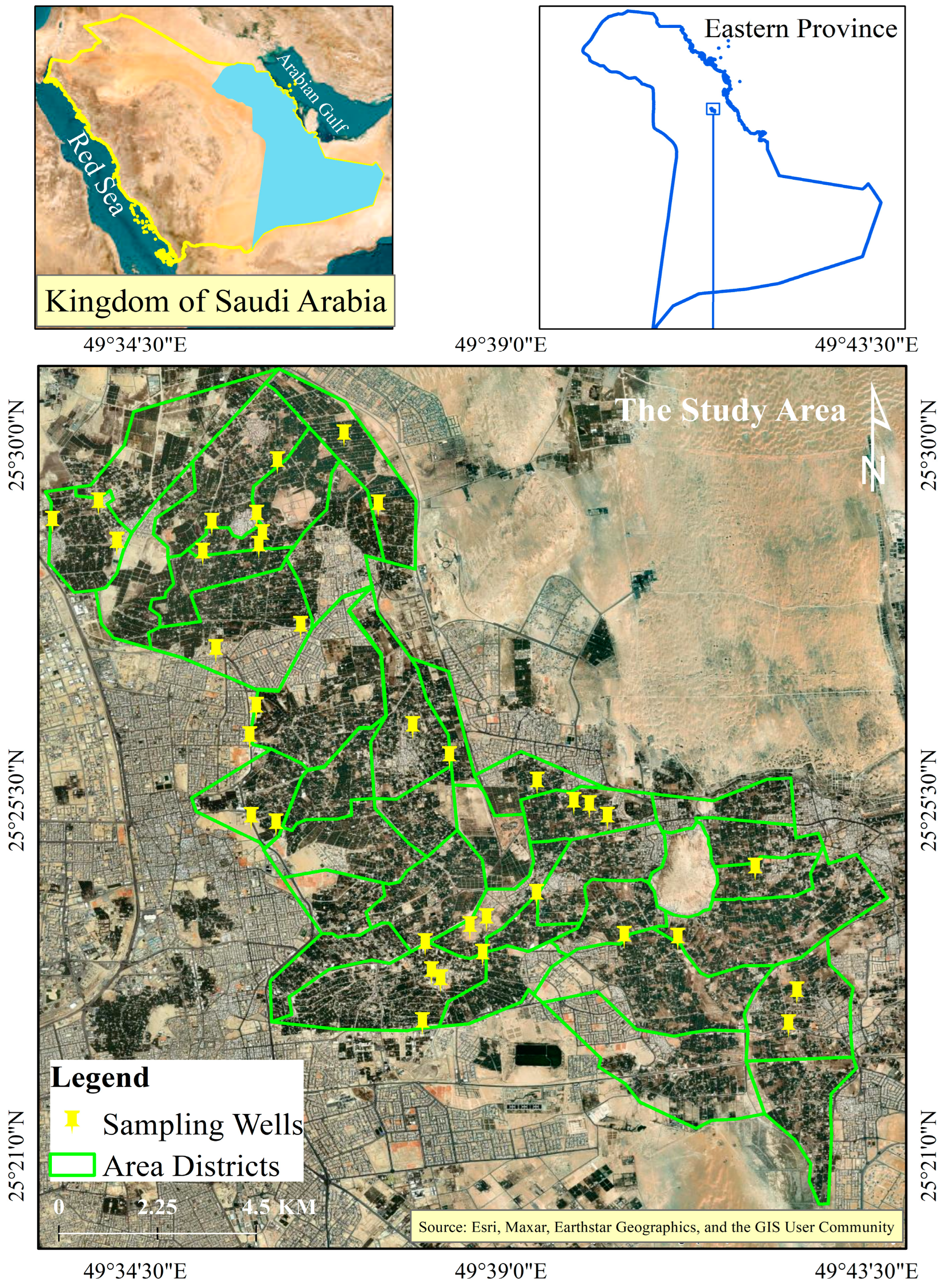
2.1. The Study Area

The large oasis of the Al-Ahsa extends over the eastern part of the Kingdome of Saudi Arabia lands; it is situated nearly 70 km inland of the Arabian Gulf coast between latitudes of 25.2° N–25.8° N and longitudes of 49.2° E–50.0° E, and is approximately 130–160 m above sea level. The area of the L-shaped oasis is approximately 20,000 ha, and is actually a composition of two connected oases [36]. The water sources used domestically as well as for irrigation are mostly supplied from the Neogene groundwater aquifer. Geologically, the oasis area is part of the Arabian Shelf in which Cenozoic as well as Mesozoic strata sequences incline mildly eastward, with a slope of about 1.0 m head for each 1 km of distance [37].
Of the pre-stated size of the Al-Ahsa area, over 8200 ha is irrigated land supporting diverse agriculture. Notably, 92% is dedicated to date palm cultivation, planted at a standard 6 m × 6 m spacing [38]. The remaining interspaces, based on available space, are utilized for a diversified mix of fruits, vegetables, or field crops. Notably, surveys across these farms have identified over 40 distinct date palm cultivars, highlighting the rich biodiversity within this cultural and economic cornerstone of the oasis. Throughout the entire Al-Ahsa area, about 336 wells have been recorded, in which, the depths of water in some wells varies between 100–180 m [39].
As part of the Al-Ahsa Oasis, the study area is situated between latitudes of 25.3° N–25.5° N and longitudes of 49.5° E–49.7° E (Figure 1), covering an approximate area of 12,892 km2. The selected study area was divided into sectors following the layouts and extensions of the most apparent districts, which are distinguished from each other by farm sizes. However, a resemblance in green surface cover dominates all of the sectors. Thus, throughout the sectors’ farms, 50 irrigation water wells were identified and spatially geocoded, and then water samples were collected for quality measurement purposes.

2.2. Collection and Preparation of Data

2.2.1. Field Data Collection

Water samples were collected in 2019 from 50 wells set for irrigation, where the wells were unsystematically scattered throughout the study area across 37 districts. The unsystematic collection of the tested wells was carried out with the purpose of approximately representing the entire area’s groundwater status. Water samples from wells that were collected and analyzed in 2019 were taken with the aim of testing the cumulative consequence of saline water on the condition of vegetation in the region during the study period, and linking this to the plant performance through assessing the VCI calculated for the same period. A Trimble-GeoXH global positioning device was used for geocoding for geographical analysis and mapping of the wells’ locations. Thus, the collected well water samples were analyzed for EC assessment, where an average value of three replicates was considered for the final analysis of each sample. The assessed water salinity was determined via conductivity units, which were DeciSiemens per meter (dS m−1).

Saline Water Classification

Since the salinity level in irrigation water raises the need for water application, along with the crop, soil climate, and irrigation method, as well as the management practices applied, a simple description of water quality is inadequate to evaluate its potential for irrigation. Nevertheless, in order to recognize the ranks that saline water takes for which these rules are proven, it is useful to set a plan for sorting [40]. Such a taxonomy is shown in Table 1 as total salt fixation, which is usually the important quality factor that compels the usage of saline water for crop yield. Strongly tolerant floras are considered to efficiently survive if their water salinity exceeds 10 dS m−1 [40].
The soil data used in this study were classified as stated by the “World Reference Base (WRB) and the United States Department of Agriculture (USDA)” classification systems [41], so that the soil data were acquired in Geo. Tiff format with a spatial resolution of 250 m at a depth of 30 cm [source: https://www.isric.org/explore/soilgrids (accessed on 13 July 2023)].

2.2.2. Spatial Data Acquisition

The spatial analysis was conducted using five Sentinel-2A satellite images, acquired throughout five consecutive years starting from 2019 up to 2023. All acquired images were downloaded (with no charges) from the “European Space Agency’s (ESA)” Copernicus program (https://scihub.copernicus.eu/, [accessed on 31 July 2023]). The Sentinel-2A mission is intended to offer high-resolution optical Earth surface images for various applications, including environmental monitoring, land cover mapping, and agricultural management.
The applied images were sensibly selected throughout the image dry periods over the study area during specific days of correspondence (i.e., July) in order to decrease the scene variation effects as well as illumination circumstances. The images acquired with 10 m spatial resolution were preprocessed, in terms of atmospheric correction and radiometric calibration, by employing the semi-automatic classification plugin (SCP) within the environment of the open-source QGIS 3.16 software program [42]. The descriptive information regarding the acquired images is shown in Table 2. In addition, the analyzed EC data all over the area were statistically tested to record any zonal correspondence within the farm areas. According to the descriptive statistics of water EC presented in Table 2, it can be observed from the coefficient of variation (CV) that the measured EC reflected a noteworthy variation in its values.

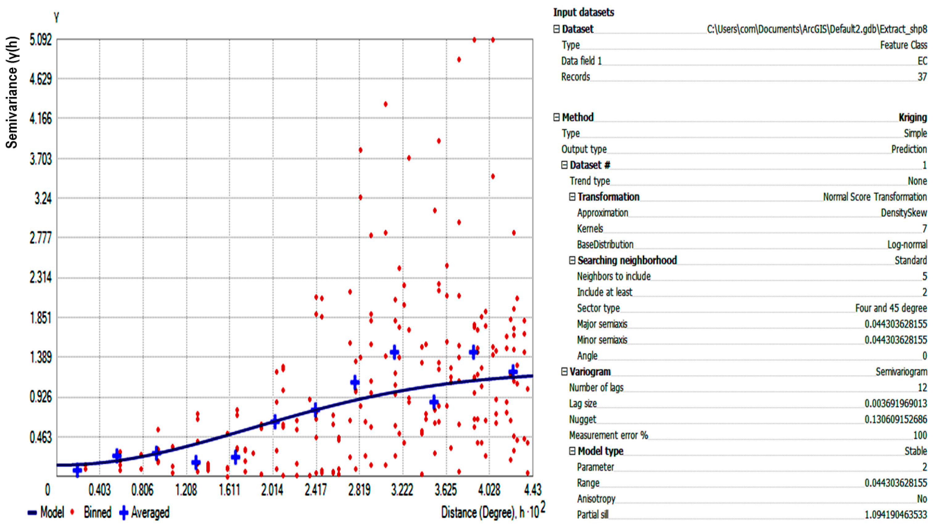
2.2.3. Spatial Data Analysis

The normalized difference vegetation index (NDVI), a broadly applied remote sensing index for measuring and monitoring vegetation health and density, was used for this study. The NDVI is calculated using the reflectance values in the near-infrared (NIR) and red bands of satellite imagery. It is worth highlighting that Sentinel-2 is one of the satellite datasets that provides suitable bands for NDVI calculation, in which the bands that correspond to near-infrared (NIR) and red (RED) are band eight and band four, respectively. Upon visualizing and interpreting the extracted NDVI image, the high values indicate healthy vegetation, and the low or negative values may represent non-vegetated surfaces, water bodies, or stressed vegetation [43]. Hence, the NDVI was calculated from the pre-stated bands by making use of the following relationship [44]:
NDVI = NIR RED NIR + RED
As all satellite images were mostly collected during the same periods in the season (day of correspondence), they could record similar spectral behavior of image pixels over the multiple years. However, this potentially emphasizes an existing spatial variability in vegetation indices triggered by other elements such as soil and irrigation water quality.
On the other hand, the VCI, a metric derived from the NDVI, is widely applied to assess the health or condition of vegetation over time. The VCI is commonly used in remote sensing and vegetation monitoring. Thus, the VCI evaluates the NDVI at the present time compared to historical values, i.e., to NDVI values at comparable periods in preceding years. It assesses the proportion of disparity within the vegetation index with regard to its extreme amplitude [45,46]. Thus, the VCI was applied in this research to characterize spatio-temporal inconsistencies in seasonal crop performance over the agricultural lands of the study area. Such inconsistencies were potentially induced by salinity variations in irrigation water, leading to the VCI being calculated as follows:
VCI = NDVI NDVI min NDVI max + NDVI min
where NDVI, NDVImin, and NDVImax are the observed, historical minimum, and historical maximum NDVI values, respectively [47].
Upon averaging the NDVI, the VCI was determined as a percentage, through applying the respective formula in Equation (2), which considers the effect of temporal change represented by the time period; this, in addition to the spatial change, takes into account the extent of the geographical correspondence between the vegetation cover and influencing factors.

2.3. Spatial and Tabular Correlation Analysis

In order to correlate vegetation performance through the VCI with EC and soil parameters, two approaches were used. First, a cross-tabulation technique was performed in the SPSS software program (IBM SPSS Version 26) to correlate the VCI, EC, and soil texture. The cross-tabulation analysis, also known as categorical variables correlation, is a statistical method used to assess the relationship between two non-continuous variables. It is often used to study the relationship between nominal variables, such as gender and occupation, or ordinal variables, such as Likert scale responses [48]. In the context of this study, cross-tabulation analysis was used to assess the relationship between the standard EC levels (ranks) and extracted levels of the VCI, given as categorical variables. On the other hand, the same analysis was also applied between the VCI and soil texture, and the latter was presented as a nominal variable.
The cross-tabulation analysis works by creating a contingency table, which is a table that shows the distribution of the two variables. The table has two rows, one for each category of one variable, and two columns, one for each category of the other variable. The number of observations in each cell of the table represents the number of observations that fall into that category combination. Once the contingency table has been created, a variety of statistical tests can be used to assess the relationship between the two variables. In this study, Somers’ d (ordinal by ordinal) and Eta (nominal by interval) correlation tests were used to evaluate the agreement between two rating variables on an ordinal scale and assess the relationship between a nominal variable and an interval one, respectively.
Second, spatial autocorrelation was used to examine the spatial associations between the VCI as a dependent variable against EC and texture variables. The bivariate local indicator of spatial autocorrelation (BiLISA) was employed to determine the degree of correlation, clustering, and significance of grid-based values, in which each grid was represented by a specific district within the study area. Further, each grid showed an average value of the VCI pixels, the well’s EC, and soil texture pixels that were geographically designated to the specific district. The BiLISA approach developed by a statistical analyst [49] involves two separate formulae, one for the bivariate local indicator of spatial association (LISA) and another for the bivariate Moran’s I statistic. However, in this study, the bivariate local indicator of spatial association (LISA) was employed to map the nature of the spatial correspondence between EC, the VCI, and texture variables, taking into account the LISA as a spatial statistics model; it combines similarity measures, which compare the actual data values between two locations, and also the spatial weight, which considers how geographically close or connected two locations are. By combining these, the LISA provides a localized picture of spatial patterns and their link to the bigger picture. Thus, for a spatial variable (i), the simplified form of the LISA can be expressed by the following equation [50]:
BiLISA i = data i   average   neighbor   data × ( neighbor   data     average   neighbor   data ) ×   spatial   weight
Employing the BiLISA, a robust spatial autocorrelation technique surpasses bivariate correlation to illuminate the complicated spatial dynamics between vegetation health and groundwater salinity. The resultant map reveals a quartet of distinct spatial signatures: “high–high and low–low” clusters, which correspond to values bordered by adjacent pixels with similar values. The other two collections represent spatial outliers (high– low and low–high), which are typically associated with values whose adjacent pixels are dissimilar. On the other hand, the conditional plot process of the three spatially correlated variables was also applied. The conditional plots in GeoDa are a type of multivariate visualization that allows users to explore the relationships between three or four variables. They are created by dividing the data into subsets based on the values of two conditioning variables, and then creating a separate plot for each subset. This allows users to see how the distribution of one variable (the dependent variable) changes across different values of the two conditioning variables [49]. Finally, GeoDa software (Version 1.12.1.161) [51], which provides a very user-friendly environment for using and analyzing spatial data autocorrelations, was used in this search.
It is also worth highlighting that the mapping of the collected and analyzed EC values was conducted using kriging’s spatial interpolator tool provided within the ArcGIS 10.8 software environment.

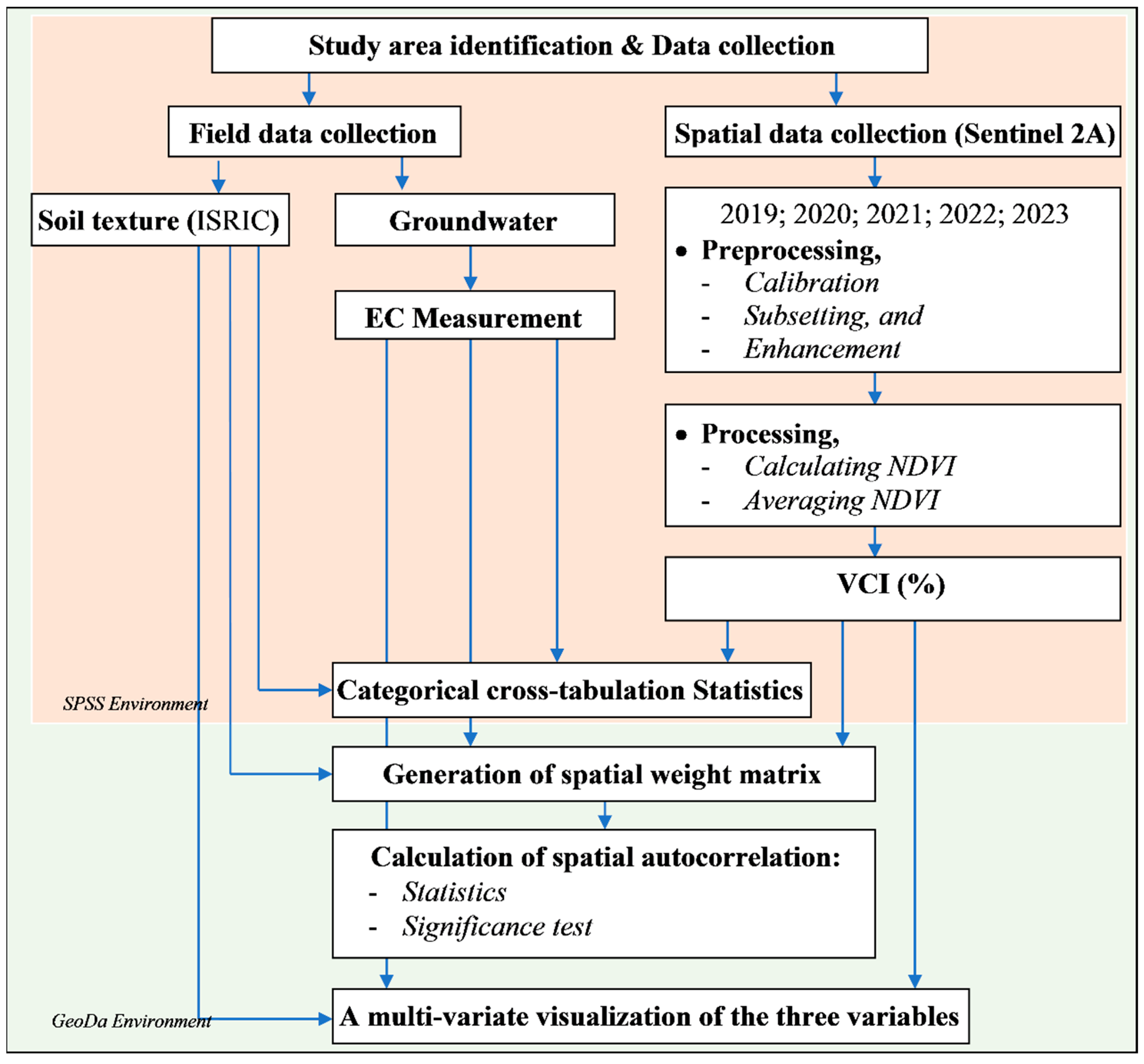
2.4. Presentation of the Work Flow

The simplified flow chart in Figure 2 shows the steps involved in assessing the spatial correlation among the vegetation performance (VCI), groundwater EC, and soil texture within the study area. The process encompassed image acquisition and preprocessing of Sentinel-2A satellite data, followed by NDVI extraction, soil data acquisition, groundwater collection, and analysis for EC. Finally, spatial autocorrelation analysis was performed.

3. Results

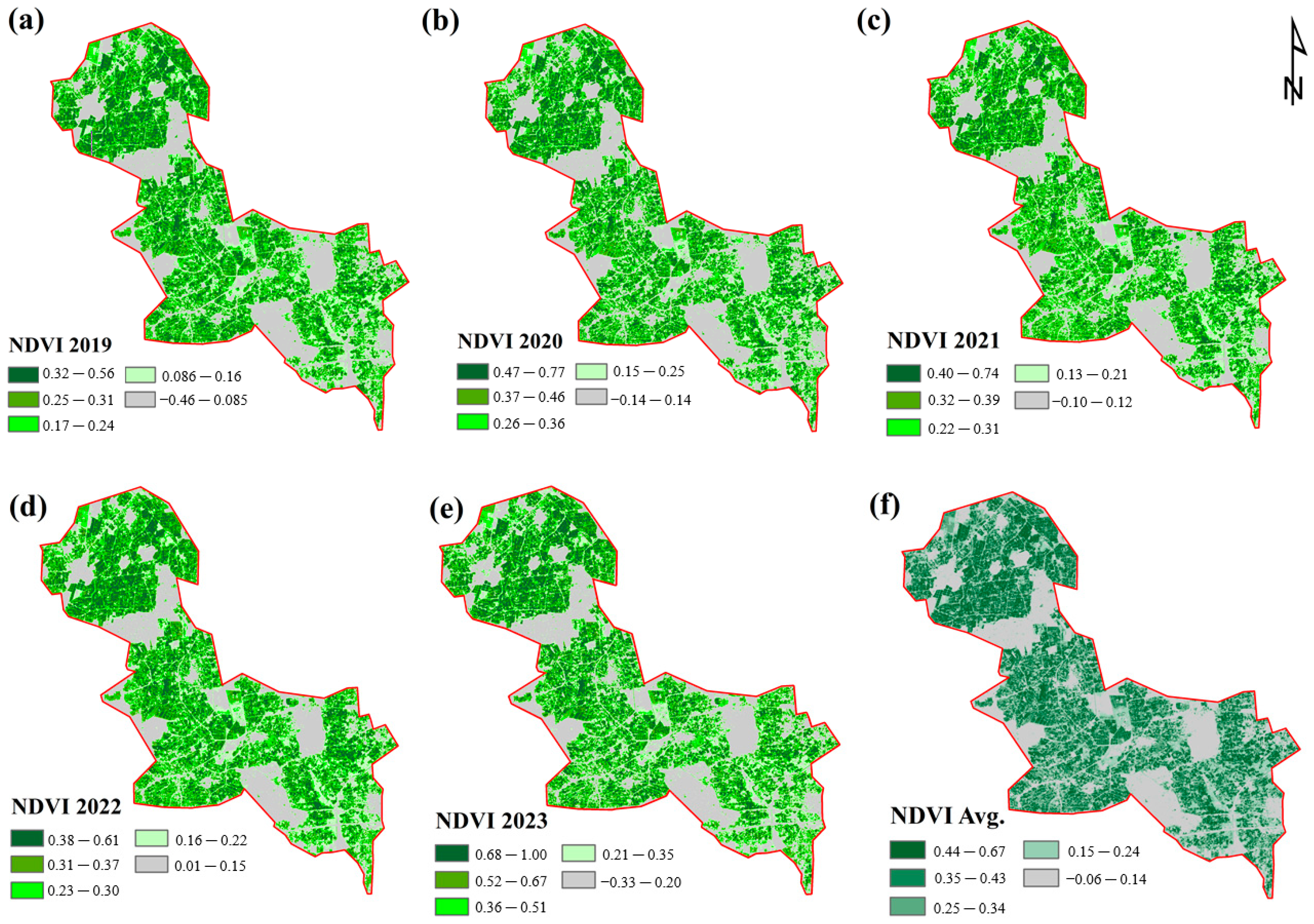
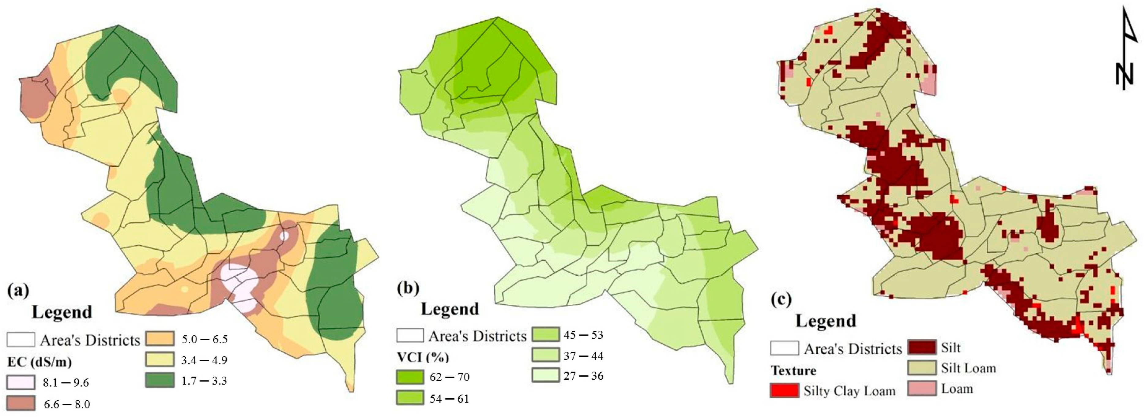
3.1. Spatial and Field Data Mapping

The extraction of surface cover NDVI information throughout the stated study periods involved utilizing the pre-stated formula (Equation (1)) to analyze the images’ red and infrared bands, in order to depict the vigor of the vegetation over the study area. Figure 3a–e represent the extracted NDVI values for the measurement years 2019, 2020, 2021, 2022 and 2023, respectively. As a result of the calculated NDVI, the average NDVI was calculated accordingly, as shown in Figure 3f. This was carried out along with identifying the observed historical minimum and historical maximum NDVI values for the purpose of assessing the VCI. As can be seen from the map, the average NDVI appears to present varying values ranging between −0.06 and 0.67, which indicates the existence of other non-vegetative surface cover types within the area (i.e., bare soils, rocks, sparse vegetation, moderate vegetation, etc.).
Through the general distribution of the VCI, it was found that VCI values within the study area ranged between 27% and 70%. The highest VCI values (70%) were concentrated over the northern oasis areas, followed by a strip at the eastern border of the oasis. This may indicate the quality of vegetation cover over these areas. In contrast, the southwestern parts of the study area witnessed the lowest VCI rates.
The resultant model’s specifications of the kriging interpolation are shown in Figure 4, for which the semivariogram was produced, which plays a critical role in quantifying the spatial autocorrelation by revealing how spatially correlated data points are. This was done by estimating the average squared difference in their values based on their separation distance. The X-axis represents the separation distance between paired data points used to calculate the semivariogram (Distance (h)), while the Y-axis represents half the average squared difference between data points separated by distance h (semivariance (γ(h)). Thus, this was carried out, in addition to identifying the spatial structure in terms of revealing the nugget, range, and sill, which were measured in the EC interpolation model as 0.13061, 0.0443 and 1.0942, respectively.
It is worth noting that the spatial distribution of groundwater salinity completely contradicted the spatial distribution of the resulting VCI, as the highest EC values, which were measured to reach 8.0–9.6 dS m−1, were concentrated within the southwestern part of the study area. In addition to some scattered spots distributed in western locations of the study area, the lowest EC values, which were measured at 1.7–3.3 dS m−1, were centered around the northern regions as well as the eastern border strip. Figure 5a shows the measured groundwater EC distribution over the study area, while Figure 5b shows the resultant VCI extracted from the five-year spatial data and Figure 5c represents the spatial distribution of the area’s soil texture measured at a depth of 30 cm as per ISRIC.

3.2. Tabulating the Spatial Correspondences

Table 3 reveals a significant association between groundwater electrical conductivity (EC) and the vegetation condition index (VCI), aligned with established salinity classifications [40]. Notably, 71% and 28.6% of the VCI were classified as “good” and “normal” conditions, respectively, which spatially corresponded with groundwater categorized as “slightly saline”. This suggests a potential link between slightly saline groundwater and healthy vegetation within the study area. Meanwhile, none of the “dry” and “extremely dry” ranks of the VCI were designated to this EC level. On the other hand, the “moderately saline” portion of the groundwater, which had a relatively wide range (2–10 dS m−1), showed relatively equivalent correspondences with the “good condition”, “normal condition”, and “dry” VCI values.
Considering the tabulated correlation between the VCI and soil texture, it can be observed from Table 3 that the higher VCI rank “good condition” had a relatively tighter correspondence (40%) to the “silt loam” portion of area soils. On the other hand, there was a complete absence of this VCI’s higher rank within the “silty clay loam” portion of the study soils. Instead, only the “dry” and “normal condition” ranks of the VCI were designated to the “silty clay loam” soil.
Furthermore, Somers’ d and Eta tests were employed to assess the goodness of fit and independence of the correlated variables. The corresponding results are presented in Table 4, which reveals statistically significant relationships between the distributions of groundwater EC, the VCI distributions, and soil texture parameters. The EC–VCI relationship was characterized by Somers’ d value of −0.53 (for VCI as dependent), with a statistical significance with p-values of 0.09. Moreover, the VCI–texture relationship was characterized by an Eta value of 0.13 (for VCI as the dependent).

3.3. Representation of Data Spatial Autocorrelation

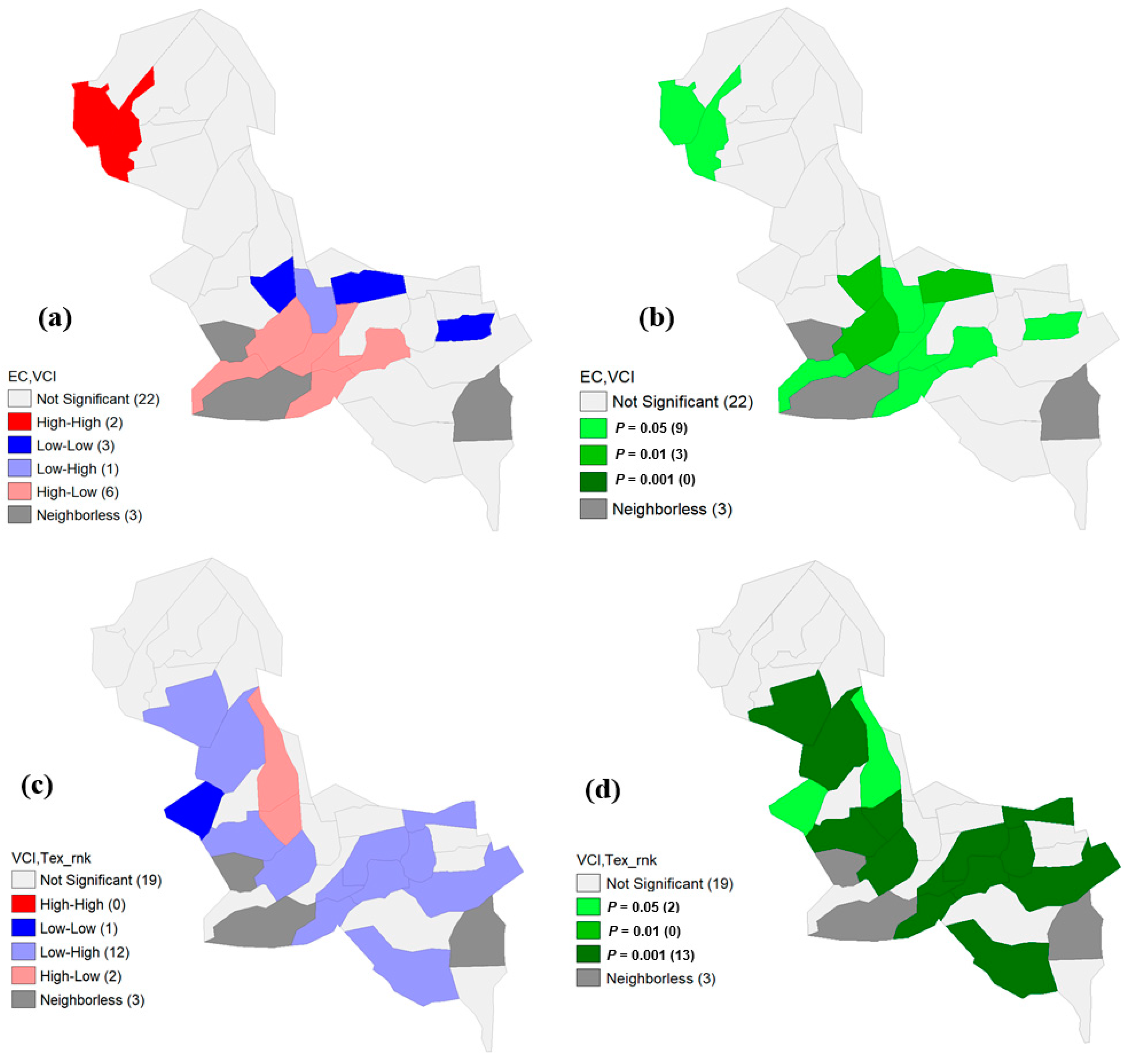
3.3.1. The Applied BiLISA Approach

The BiLISA method was employed to investigate any potential patterns of correlation within the VCI spatial distribution, groundwater EC, and soil texture. Figure 6 presents two forms of BiLISA application to the spatial parameters, which are EC-VCI and VCI–texture autocorrelations, supported with their relative significance maps produced accordingly. The resultant clustering map (Figure 6a), which was between EC (independent) and VCI (dependent), revealed significant clustering of high EC values associated with low VCI, centered over the middle to the west of the study area. This spatial association was confirmed and is depicted through a significance map in Figure 6b, in which p-values of 0.05 to 0.01 were measured. Nevertheless, few districts located to the east and north-west of the area demonstrated outlier values represented by the existence of high and low EC values that were spatially associated with high and low VCI values, respectively.
On the other hand, based on the classification of soil texture types via the USDA [41], a spatial autocorrelation was plotted between the VCI and the classes of soil texture. This was conducted utilizing USDA soil texture classes as alternatives to the nominal context (in order to adapt to the spatial analysis environment). Hence, as only “silt” as well as “silt loam” soil textures were dominant over the study site, silt was assigned the order “high”, while silt loam was assigned the order “low”; then, the texture classes were spatially autocorrelated against the VCI. The resultant BiLISA of VCI–texture in Figure 6c shows significant clustering of low VCI values that spatially corresponded to the silt soil texture over the middle to the west, in addition to some parts at the south of the study area in which a significant p-value of 0.001 was observed. This spatial status of the VCI being a dependent variable influenced by soil texture is in line with the VCI–EC relationship.

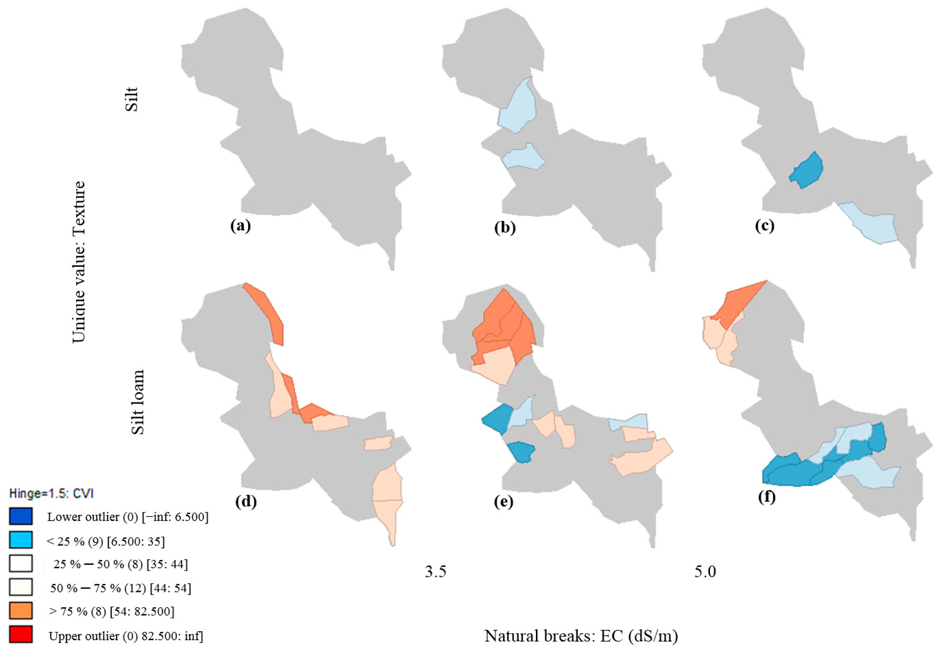
3.3.2. EC Centralization Effect (the Conditional Plot Maps)

The resultant conditional plot in Figure 7 shows that there is a strong relationship between groundwater EC, soil texture, and surface VCI, in which the lower VCI outlier (lower VCI values) spatially correlates with the highest EC values (above 5 dS m−1) over the “silt loam” soils over the middle to the west of the study area (Figure 7f). In contrast, the upper outlier (higher VCI values) spatially corresponds to the lower EC values, which are mostly centered over the eastern (Figure 7d) and northern (Figure 7e) portions of the study area. However, the “silt” class of the area soils did not show a noticeable trend for the three-variable relationship (Figure 7a–c).
Overall, the relationship between water salinity, soil texture, and vegetation condition is complex, with each factor influencing the others in various ways. These results confirm a strong relationship among groundwater EC, VCI, and soil texture, which is consistent with the findings of previous cross-tabulation statistics.

4. Discussion

4.1. Statement of VCI, EC, and Texture Distribution

Groundwater salinity is a major concern in the Al-Ahsa region of Saudi Arabia, as it can significantly influence agriculture, ecosystems, and human health. Basically, the depicted spatial distribution in groundwater salinity over the study area (Figure 5a) is justifiable by the fact that extensive groundwater exploitation activities have been carried out within the mid-west districts of the oasis. This in itself can be justified by the high number of farms in this area compared to the north of the oasis, where the farm area is larger compared to their numbers; thus, a small number of underground wells are used. Hence, the relationship between salinity and vegetation performance vitally indicates that the VCI could depict the status of green cover and its tolerance to the quality of irrigation water, especially since the measurement period, which is five years, was identical between the two variables.
The presented data paint a nuanced picture of the study area’s vegetation health and groundwater salinity, revealing both spatial heterogeneity and potential causal relationships. The VCI distribution further corroborated this spatial disparity, so that the highest values (60–70%) concentrated in the north and east suggest optimal vegetation conditions. Conversely, the lower VCI values (27–40%) in other parts potentially signify areas with less robust vegetation growth. This spatial pattern suggests that the oasis and eastern border zones enjoy more favorable conditions for vegetation compared to other regions.
Interestingly, the groundwater EC distribution seemingly mirrors the vegetation health pattern. The highest salinity values (8.0–9.6 dS m−1) in the southwest coincide with potentially stressed vegetation conditions (Figure 5), while the lowest salinity values (1.7–3.3 dS m−1) in the north and east align with healthy vegetation. This suggests a potential causal link between groundwater salinity and vegetation health, with higher salinity potentially affecting vegetation growth and vigor. The negative impact of high salinity on vegetation is consistent with numerous studies on agricultural landscapes and saline environments [52,53,54].
When considering the cross-tabulation result for assessing the interconnectedness between groundwater salinity, soil texture, and vegetation condition index (VCI) within the study area, the technique showed the co-occurrence of “good” and “normal” VCI with “slightly saline” groundwater again, which aligns with the pre-stated research [55,56,57]. This suggests that moderate salinity may not pose a significant threat to vegetation health in certain contexts. However, the conspicuous absence of “dry” and “extremely dry” VCI values within this category echoes the observations of Gao et al. [54], highlighting potential sensitivity to higher salinity thresholds beyond a specific tolerance range. Further, the broader spectrum of VCI values (“good”, “normal”, and “dry”) corresponding to “moderately saline” groundwater underscores the multifaceted nature of this relationship. As noted by Chen et al. [55], the impact of salinity on vegetation resilience is contextual and influenced by a constellation of additional factors beyond salinity levels alone. Soil characteristics and land management practices all play a critical role in shaping the vegetation’s response to saline stress.
On the other hand, the exclusive association of “good” VCI with “silt loam” soil texture and its complete absence in “silty clay loam” resonates with the findings of Elhag et al. [56]. This suggests that well-drained sandy loam soils, with their superior water infiltration and aeration, offer a buffer against moderate salinity compared to heavier clay-rich soils. This likely explains the presence of only “normal” and “dry” VCI values in silty clay loam, indicating its limited capacity to sustain optimal vegetation health under saline conditions. However, these findings call for further investigation into the precise mechanisms governing these intertwined relationships. Delving deeper into the combined effects of salinity, soil texture, and additional factors such as land management practices can unravel the intricacies of vegetation resilience in saline environments.

4.2. The Nature of Spatial Autocorrelation between Variables

The BiLISA analysis highlighted the complicated spatial relationships among VCI, groundwater EC, and soil texture, explaining the nature of correlations. The clustering of high EC values with low VCI in the mid-west of the oasis reinforces the intuitive expectation that saline groundwater negatively influences vegetation health. This aligns with local studies by Aldakheel [57] and Al-Rashed et al. [58], who also found negative spatial correlations between saline groundwater and vegetation health in specific parts of the oasis. This confirms the widespread challenge of salinity hindering vegetation growth in Al-Ahsa. Moreover, the presence of outlier districts with contrasting EC-VCI pairs (Figure 7) suggests local factors are at play. These areas may benefit from favorable local factors like specific land conservation practices that mitigate the negative impact of salinity on vegetation. Further investigation into these outliers could reveal crucial insights for enhancing resilience in saline environments. Furthermore, the spatial overlap between low VCI and silt soil texture in the mid-west and southern areas of the oasis highlights the critical role of soil drainage in determining plant health. Silt’s lower water-holding capacity compared to clay may lead to faster infiltration of saline groundwater, exacerbating water stress and reducing the VCI [56]. Conversely, the upper VCI outliers linked with lower EC and eastern/northern areas suggest that lower salinity and potentially more clay-rich soils (not shown for silt) create conditions conducive to healthy vegetation. Silt’s ambiguity, notably, the “silt” soil class, does not exhibit a clear trend. This suggests other factors like local hydrology or specific crop types may influence the VCI in these areas.
To sum up, the BiLISA analysis revealed a value-added mechanism of spatial dependency assessment among VCI, EC, and soil texture. It confirmed the detrimental impact of high salinity on the VCI, particularly in synergy with less favorable soil drainage. However, it also highlights the potential for local factors and soil type variations to modulate these relationships. This nuanced understanding offers valuable insights for targeted interventions, promoting resilient vegetation growth even in areas with saline groundwater challenges.
Ensuring the long-term viability of Al-Ahsa’s agricultural landscape necessitates a multi-pronged approach informed by scientific principles. Precision irrigation technologies, employing sensors and real-time data to deliver water efficiently, offer significant potential. Integrating drought-resistant crop varieties and diversified planting strategies further contribute to water conservation. On-farm practices like land leveling, canal lining, and mulching techniques further minimize water loss. Additionally, treating and reusing wastewater provides a sustainable irrigation source. Empowering farmers through educational programs and promoting efficient water use practices are vital components. Furthermore, supportive government policies, infrastructure upgrades, and targeted financial incentives can accelerate adoption of these interventions. Finally, continuous research efforts focused on drought-resistant cultivars, advanced irrigation technologies, and localized water management strategies are crucial for long-term sustainability. By implementing this collective approach, informed by science and technology, Al-Ahsa can optimize water management, minimize waste, and secure a water-efficient future for generations to come.

5. Conclusions

This study aimed to reveal the intricate spatial relationship between medium-term vegetation health, as reflected by the vegetation condition index (VCI) over a 5-year period, and groundwater salinity. The moderating role of soil texture in this relationship was further investigated, with a specific focus on explaining potential fluctuations in groundwater salinity attributable to the application of saline irrigation water. By comprehensively examining these three-way interactions, I sought to illuminate the complex impact of irrigation practices on regional water resources and vegetation dynamics. The key findings of this study include the following:
  • The vegetation health, as indicated by the VCI, exhibited significant spatial variations across the oasis. Notably, the northern and eastern oasis sectors claimed higher VCI values, indicative of robust vegetation cover, while the southwestern region demonstrated a contrasting trend with elevated groundwater salinity levels.
  • A complex relationship exists between groundwater salinity and vegetation health. While “good condition” VCI predominantly co-occurred with slightly saline groundwater and silty loam soils, moderate salinity levels (2–10 dS m−1) displayed multifaceted associations with various VCI classes.
  • BiLISA analysis revealed statistically significant clusters of both high salinity–low VCI and low salinity–high VCI, suggesting the influence of localized factors beyond simple salinity-driven effects. Furthermore, specific outlier districts shown atypical EC-VCI relationships, hinting at potentially mitigating influences such as land management practices.
  • The role of soil texture in modulating VCI responses to salinity emerged as a crucial factor. Silt loam soils demonstrated a closer association with “good condition” VCI, whereas silty clay loam primarily supported dry and normal vegetation conditions. Notably, “silt” soils exhibited an ambiguous relationship, warranting further investigation.
Briefly, these results underscore the importance of considering spatial variability when analyzing vegetation health and groundwater salinity. The study area exhibited distinct spatial patterns, with the northern and eastern regions presenting more favorable conditions compared to the southwest. However, in light of all these outcomes, there are some determinants that the study did not address, for instance, the integration of additional data on factors such as soil moisture, organic matter, and plant species composition, which can provide a more comprehensive understanding of vegetation health. Moreover, incorporating information about plant tolerances and adaptations can improve the accuracy of assessments, especially in diverse ecosystems, in addition to the fact that the influence of soil texture on vegetation can vary depending on the spatial scale of observation.
To sum up, further investigation is warranted to clarify the driving factors behind these patterns and the potentially causal relationship between salinity and vegetation health. By considering these spatial differences, targeted interventions can be implemented to optimize water management practices and enhance overall ecosystem health in the study area. Hence, advanced statistical modeling and integration of remote sensing, GIS, and social data can offer a more nuanced understanding and strengthen spatial predictions of vegetation in response to environmental challenges.

Funding

This work was supported by the Deanship of Scientific Research, Vice Presidency for Graduate Studies and Scientific Research, King Faisal University, Saudi Arabia [Grant No 5534].

Data Availability Statement

Data are available upon request from the corresponding author.

Acknowledgments

The author would like to thank King Faisal University for its continuous support and help.

Conflicts of Interest

The author declares no conflicts of interest.

References

  1. Ayers, R.S.; Westcot, D.W. Water Quality for Agriculture; Food and Agriculture Organization of the United Nations: Rome, Italy, 1989; Volume 29. [Google Scholar]
  2. Guilherme, A.; Tormena, C.A.; Rattan, L.; Leandro, Z.; Claudinei, K. Enhancing soil physical quality and cotton yields through diversification of agricultural practices in central Brazil. Land Degrad Develop. 2019, 30, 788–798. [Google Scholar]
  3. Shrivastava, P.; Kumar, R. Soil salinity: A serious environmental issue and plant growth promoting bacteria as one of the tools for its alleviation. Saudi J. Biol. Sci. 2015, 22, 123–131. [Google Scholar] [CrossRef] [PubMed]
  4. FAO. Food and Agriculture Organization’s Handbook for Saline Soil Management. 2018. Available online: https://www.fao.org/publications (accessed on 4 December 2018).
  5. Dong, H. Combating salinity stress effects on cotton with agronomic practices. Afric. J. Agric. Res. 2012, 7, 4708–4715. [Google Scholar] [CrossRef]
  6. Munns, R. Comparative physiology of salt and water stress. Plant Cell Environ. 2002, 25, 239–250. [Google Scholar] [CrossRef] [PubMed]
  7. Tang, W.; Luo, Z.; Wen, S.; Dong, H.; Xin, C.; Li, W. Comparison of inhibitory effects on leaf photosynthesis in cotton seedlings between drought and salinity stress. Cotton Sci. 2007, 19, 28–32. [Google Scholar]
  8. Edelstein, M.; Plaut, Z.; Ben-Hur, M. Water salinity and sodicity effects on soil structure and hydraulic properties. Adv. Hortic. Sci. 2010, 24, 154–160. [Google Scholar]
  9. Nxele, X.; Klein, E.; Ndimba, B.K. Drought and salinity stress alters ROS accumulation, water retention and osmolyte content in sorghum plants. S. Af. J. Bot. 2017, 108, 261–266. [Google Scholar] [CrossRef]
  10. Carillo, P.; Maria, G.A.; Giovanni, P.; Amodio, F.; Pasqualina, W. Salinity Stress and Salt Tolerance, Abiotic Stress in Plants—Mechanisms and Adaptations; Shanker, A., Ed.; InTech: London, UK, 2011; Available online: https://www.intechopen.com/books/abioticstress-in-plants-mechanisms-and-adaptations/salinity-stress-and-salt-tolerance (accessed on 10 March 2020).
  11. Al-Omran, A.M.; Aly, A.; Al-Wabel, M.; Sallam, A.; Al-Shayaa, M. Hydrochemical characterization of groundwater under agricultural land in arid environment: A case study of Al-Kharj, Saudi Arabia. Arab. J. Geosci. 2016, 9, 68–85. [Google Scholar] [CrossRef]
  12. Al-Omran, A.; Aly, A.; Al-Wabel, M.I.; Al-Shayaa, M.S.; Sallam, A.S.; Nadeem, M.E. Geostatistical methods in evaluating spatial variability of groundwater quality in Al-Kharj Region, Saudi Arabia. Appl. Water Sci. 2017, 7, 4013–4023. [Google Scholar] [CrossRef]
  13. Al-Omran, A.M.; Awad, M.; Alharbi, M.; Nadeem, M. Hydrogeochemical characterization and groundwater quality assessment in Al-Hasa, Saudi Arabia. Arab. J. Geosci. 2018, 11, 79. [Google Scholar] [CrossRef]
  14. El-Mahmoudi, A.; Hussein, M. Geochemical modeling of groundwater salinization in Al-Ahsa Oasis, Saudi Arabia. Environ. Process. 2017, 4, 509–532. [Google Scholar]
  15. Aly, A.A.; Hussain, F.M.; Abd El-Moez, S.R. Assessment of groundwater quality in Al-Ahsa Oasis, Saudi Arabia using multivariate statistical analysis and GIS techniques. Environ. Earth Sci. 2013, 70, 3967–3992. [Google Scholar]
  16. Al-Zarah, A.I. Hydrochemistry and environmental significance of groundwater in Al-Ahsa Oasis, Saudi Arabia. Environ. Earth Sci. 2008, 56, 1607–1618. [Google Scholar]
  17. Al-Ahmadi, M. The impact of climate change on the water resources of Saudi Arabia. J. King Saud Univ.-Sci. 2010, 22, 207–217. [Google Scholar]
  18. Al-Jaber, F.; Ghulam, A. Estimation of potential and open water evaporation in arid regions using ERA-Interim reanalysis data. Arab. J. Geosci. 2014, 7, 3263–3270. [Google Scholar]
  19. Amer, M.A.; Hassan, F.A. Irrigation with treated wastewater and impact on soil properties in Al-Ahsa Oasis, Saudi Arabia. Agric. Water Manag. 2008, 95, 801–806. [Google Scholar]
  20. Bakhit, M.K.; Al-Ahmadi, M.A.; Al-Ghamdi, A.S. Numerical modeling of seawater intrusion in the eastern coast of Al-Ahsa Oasis, Saudi Arabia. J. King Saud Univ.-Sci. 2017, 29, 309–321. [Google Scholar]
  21. Todd, D.K.; Mays, L.W. Groundwater Hydrology, 3rd ed.; John Wiley & Sons: Hoboken, NJ, USA, 2005. [Google Scholar]
  22. Fetter, C.W. Applied Hydrogeology, 4th ed.; Prentice Hall: Upper Saddle River, NJ, USA, 2001. [Google Scholar]
  23. Bear, J.; Verruijt, A. Modeling Groundwater Flow and Pollution; D. Reidel Publishing Company: Dordrecht, The Netherlands, 1987. [Google Scholar]
  24. Allbed, A.; Kumar, L. Soil salinity and vegetation cover change detection from multi-temporal remotely sensed imagery in Al Hassa Oasis in Saudi Arabia. Environ. Earth Sci. 2016, 70, 3967–3992. [Google Scholar] [CrossRef]
  25. Menenti, M.; Van Deursen, W.; De Haan, F.J. Satellite-based detection of changes in surface water quality. Int. J. Remote Sens. 1986, 7, 1437–1454. [Google Scholar]
  26. Madani, K. Land salinization mapping in arid regions using remote sensing techniques. J. Indian Soc. Remote Sens. 2005, 33, 309–316. [Google Scholar]
  27. Shrestha, M.B. Landsat-based estimates of soil salinity in the Terai Region of Nepal. Int. J. Remote Sens. 2006, 27, 3703–3715. [Google Scholar]
  28. Bannari, A.; Guedira, M.; Hajab, E.L.; Omasa, K.; Kawamura, H. Monitoring and spatial modeling of soil salinity in irrigated areas using a spectral index derived from landsat-5 TM imagery. Int. J. Remote Sens. 2008, 29, 6603–6624. [Google Scholar]
  29. Allbed, A.; Kumar, L.; Aldakheel, Y.Y. Mapping of soil salinity using landsat data and support vector machines in Al-Hassa Oasis, Saudi Arabia. Arab. J. Geosci. 2014, 7, 3269–3282. [Google Scholar]
  30. Fernández-Buces, A.; Camacho-Ordoñez, C.; Plaza, A.; García-Haro, F.J. Spectral indices for the automatic recognition of saline areas in imagery-based irrigation management. Agron. J. 2006, 98, 720–729. [Google Scholar]
  31. Lobell, D.B.; Asner, G.P.; Heilman, C.M.; Baez, S. Remote sensing of regional crop yield variability. Proc. Natl. Acad. Sci. USA 2010, 107, 20924–20929. [Google Scholar]
  32. Al-Mulla, M.M.; Al-Adawi, S.S. Temporal changes in soil salinity mapping using remote sensing and GIS techniques in the Al-Rumais region, Oman. Environ. Monit. Assess. 2009, 159, 309–320. [Google Scholar]
  33. Tripathi, N.K.; Rao, A.R.; Sharma, R.A. Mapping of soil salinity using remote sensing. Int. J. Remote Sens. 1997, 18, 2909–2915. [Google Scholar]
  34. Al-Khaier, F. Application of remote sensing techniques for the detection of soil salinity in arid and semi-arid regions. Adv. Space Res. 2003, 32, 1423–1430. [Google Scholar]
  35. Nield, A.A.; Running, S.W.; Gowda, S.H. Remote sensing of soil salinity in the Colorado River Basin. Remote Sens. Environ. 2007, 109, 354–364. [Google Scholar]
  36. Al-Naeem, A.A. Evaluation of groundwater of al-hassa oasis, eastern region Saudi Arabia. Res. J. Environ. Sci. 2011, 5, 624–642. [Google Scholar]
  37. Al-Sayari, S.; Zott, J.G. Quaternary Period in Saudi Arabia; Springer: Wien, NY, USA, 1978. [Google Scholar]
  38. Elprince, A.M.; Makki, Y.M.; Al-Barrak, S.A.; Tamim, T.M. Use of Computer Graphics in developing density maps for the date culture of Al-Hassa oasis in Saudi Arabia. In Proceedings of the First Symposium on Date Palm Conference, Al-Hassa, Saudi Arabia, 23–25 March 1982; pp. 674–682. [Google Scholar]
  39. Wakuti. Studies for the Project of Improving Irrigation and Drainage in the Region of al-Hassa, Saudi Arabia; Soil Study: Siegen, Germany, 1969; p. 3. [Google Scholar]
  40. Rhoades, J.D.; Kandiah, A.; Mashali, A.M. The Use of Saline Waters for Crop Production FAO irrigation and Drainage Paper; FAO: Rome, Italy, 1992; p. 48. [Google Scholar]
  41. Hengl, T.; Mendes de Jesus, J.; Heuvelink, G.B.M.; Ruiperez Gonzalez, M.; Kilibarda, M.; Blagotić, A.; Shangguan, W.; Wright, M.N.; Geng, X.; Bauer-Marschallinger, B.; et al. SoilGrids250m: Global gridded soil information based on machine learning. PLoS ONE 2017, 12, e0169748. [Google Scholar] [CrossRef]
  42. Congedo, L. Semi-automatic classification plugin documentation. Release 2016, 3, 29. [Google Scholar]
  43. Silleos, N.G.; Alexandridis, T.K.; Gitas, I.Z.; Perakis, K. Vegetation indices: Advances made in biomass estimation and vegeta-tion monitoring in the last 30 years. Geocarto. Int. 2006, 21, 21–28. [Google Scholar] [CrossRef]
  44. Johansen, B.; Tømmervik, H. The relationship between phytomass, NDVI and vegetation communities on Svalbard. Int. J. Appl. Earth Obs. Geoinf. 2014, 27, 20–30. [Google Scholar] [CrossRef]
  45. Du, L.; Tian, Q.; Yu, T.; Meng, Q.; Jancso, T.; Udvardy, P.; Huang, Y. A Comprehensive Drought Monitoring Method Integrating MODIS and TRMM Data. Int. J. Appl. Earth Obs. Geoinf. 2013, 23, 245–253. [Google Scholar] [CrossRef]
  46. Zhuo, Z.Y.; Long, Q.B.; Bai, P. Scale of Meteorological Drought Index Suitable for Characterizing Agricultural Drought: A Case Study of Hunan Province. J. South-to-North Water Transf. Water Sci. Technol. 2021, 19, 119–128. [Google Scholar]
  47. Kogan, F.N.; Gitelson, A.; Edige, Z.; Spivak, I.; Lebed, L. AVHRR-based spectral vegetation index for quantitative assessment of vegetation state and productivity: Calibration and validation. Photogramm. Eng. Remote Sens. 2003, 69, 899–906. [Google Scholar] [CrossRef]
  48. Myers, J.L.; Well, A.D. Research Design and Statistical Analysis, 2nd ed.; Erlbaum: Lawrence, KS, USA, 2003; p. 508. ISBN 978-0-8058-4037-7. [Google Scholar]
  49. Anselin, L. Exploring Spatial Data with GeoDa: A Workbook; Center for Spatially Integrated Social Science, University of Illinois: Urbana, IL, USA, 2015; p. 61801. [Google Scholar]
  50. Anselin, L. Spatial regression in a multivariate framework. Spat. Anal. Geogr. Inf. Syst. 1995, 1, 31–52. [Google Scholar]
  51. Anselin, L.; Syabri, I.; Kho, Y. GeoDa: An introduction to spatial data analysis. Geogr. Anal. 2006, 38, 5–22. [Google Scholar] [CrossRef]
  52. Jamil, A.; Ahmad, R.; Qadir, M. Relationship between soil salinity and vegetation indices in agricultural landscapes of Punjab, Pakistan. Remote Sens. Lett. 2023, 14, 749–755. [Google Scholar]
  53. Qiu, L.; Zhang, X.; Zhao, X.; Yang, Z.; Zhang, Z. Exploring the influence of soil salinity on maize vegetation indices and yield using sentinel-2 and sentinel-1 data. Remote Sens. 2022, 14, 1696. [Google Scholar] [CrossRef]
  54. Gao, J.; Xu, W.; Zhao, H.; Yang, D.; Wang, R. Spatiotemporal changes in soil salinity and their impacts on vegetation greenness in irrigated agricultural land using Sentinel-2 data. Remote Sens. Environ. 2023, 282, 111305. [Google Scholar]
  55. Chen, X.; Cui, X.; Zhao, Z.; Chen, B.; Li, R. Spatiotemporal analysis of land salinization and its impact on vegetation coverage in the Ebinur Lake Basin, China. Remote Sens. 2022, 14, 4005. [Google Scholar] [CrossRef]
  56. Elhag, A.M.; Al-Barakati, F. A hybrid approach for vegetation condition monitoring, groundwater salinity and land degradation detection in the coastal arid region of Saudi Arabia. Sustain. Ecosyst. Resour. 2021, 10, 1567–1584. [Google Scholar]
  57. Aldakheel, A.A. Soil salinity as a selection pressure is a key determinant for the presence of halophytes in Al-Ahsa Oasis, Eastern Saudi Arabia. Saudi J. Biol. Sci. 2010, 17, 191–196. [Google Scholar] [CrossRef]
  58. Al-Rashed, M.M.; Elhag, M.; Al-Barakati, F. Assessing land degradation and desertification risks in Al-Ahsa Oasis, Saudi Arabia, using GIS techniques. Appl. Ecol. Environ. Res. 2017, 15, 703–724. [Google Scholar]
Figure 1. Study area layout, in which sampling locations are delineated.
Water 16 00643 g001
Figure 2. Flow chart of the applied cross-tabulation and spatial autocorrelation procedures.
Water 16 00643 g002
Figure 3. Representation of NDVI data extracted for five years, namely, (a) 2019, (b) 2020, (c) 2021, (d) 2022 and (e) 2023. These images are presented along with their (f) calculated average value. It can be observed that the spatial variation of the vegetation cover within the single landscape was more influential than the temporal variation during the years that the study was conducted. This confirms that the geographical distribution of groundwater quality in the study area may have played an effective role in the distribution of vegetation cover.
Water 16 00643 g003
Figure 4. Presentation of the resultant kriging model’s specifications, in which the kriging semivariogram chart depicts the spatial relationship between points in the dataset, focusing on how variability changes with distance. The input dataset on the right pane provides information on the analyzed data size, method type and nature of output, and variogram and model types.
Water 16 00643 g004
Figure 5. The groundwater-measured salinity given as (a) EC dS m−1, the green surface cover status represented by (b) VCI, and (c) soil texture classes.
Water 16 00643 g005
Figure 6. The bivariate local indicator of spatial association (BiLISA) for (a) EC-VCI variables with their related (b) significance map, in addition to the (c) VCI–texture relationship confirmed with their (d) significance map.s.
Water 16 00643 g006
Figure 7. EC centralization effect analysis through plotting EC, VCI, and soil texture. The given plots are representations of (a) lower EC within “Silt” soil, (b) medium EC within “Silt” soil, (c) higher EC within “Silt” soil, (d) lower EC within “Silt loam” soil, (e) medium EC within “Silt loam” soil, and (f) higher EC within “Silt loam” soil.
Water 16 00643 g007
Table 1. Salinity taxonomy for water according to (FAO) recommendations [source: [40]].
Class of Water EC (dS/m)Concentration of Salts (mg/L)Water Category
No salinity<0.7<500Drinking as well as irrigation
Slight salinity0.7–2500–1500Irrigation
Moderate salinity2–101500–7000Main drainage water/groundwater
Highly saline10–257000–15,000Secondary drainage water/groundwater
Very High salinity25–4515,000–35,000Very saline groundwater
Brine >45>35,000Seawater
Table 2. Specifications and statistics of the acquired Sentinel-2A images and collected EC samples.
Type of Data Date of Data Attainment Data SpecificationsData Source
Satellite imagery [Sentinel-2A]201919 JulyPath/row: 164/42
Spectral bands: 12 channels
Pixel size: 10 m (for RGB bands)
Revisit frequency (days): 5
The European Space Agency’s (ESA) Copernicus program
20203 July
202123 July
202218 July
20238 July
Soil texture2023Format: Geo. Tiff.
Resolution: 250 m at 30 cm depth.
Coordinate reference system: EPSG: 4326.
The International Soil Reference and Information Centre (ISRIC)
Collected EC data (dS m−1)
Max9.60This statistical representation is based on 50-wells sample size.
Min1.79
Avg.4.47
STD1.34
CV0.30
Table 3. EC (dS m−1) and texture versus VCI categories cross-tabulation.
VCI CategoriesTotal
Extremely Dry (0–20%)Dry (20–40%)Normal Condition (40–60%)Good Condition (60–80%)
EC (dS m−1) CategoriesSlightly saline (0.7–2)Count00257
% within EC Categories0.0%0.0%28.6%71.4%100.0%
Moderately saline (2–10)Count414121343
% within EC Categories9.3%32.6%27.9%30.2%100.0%
TotalCount414141850
% within EC Categories8.0%28.0%28.0%36.0%100.0%
TextureSilty clay loamCount02204
% within Texture0.0%50.0%50.0%0.0%100.0%
Silt Count12339
% within Texture11.1%22.2%33.3%33.3%100.0%
Silt loamCount31091537
% within Texture8.1%27.0%24.3%40.5%100.0%
TotalCount414141850
% within Texture8.0%28.0%28.0%36.0%100.0%
Table 4. Correlation tests of Somers’ d (ordinal by ordinal) and Eta (nominal by interval).
TestsSymmetricValueApproximate Significance
Ordinal by OrdinalSomers’ d CorrelationVCI Category Dependent−0.5320.009
Nominal by IntervalEtaVCI Category Dependent0.131
N of Valid Cases50
Disclaimer/Publisher’s Note: The statements, opinions and data contained in all publications are solely those of the individual author(s) and contributor(s) and not of MDPI and/or the editor(s). MDPI and/or the editor(s) disclaim responsibility for any injury to people or property resulting from any ideas, methods, instructions or products referred to in the content.

