Abstract
Traditional hydrodynamic models face the significant challenge of balancing the demands of long prediction spans and precise boundary conditions, large computational areas, and low computational costs when attempting to rapidly and accurately predict the nonlinear spatial and temporal characteristics of fluids at the basin scale. To tackle this obstacle, this study constructed a novel deep learning framework with a hydrodynamic model for the rapid spatiotemporal prediction of hydrodynamics at the basin scale, named U-Net-ConvLSTM. A validated high-fidelity hydrodynamic mechanistic model was utilized to build a 20-year hydrodynamic indicator dataset of the middle and lower reaches of the Han River for the training and validation of U-Net-ConvLSTM. The findings indicate that the value of the model surpassed 0.99 when comparing the single-step prediction results with the target values. Additionally, the required computing time fell by 62.08% compared with the hydrodynamic model. The ablation tests demonstrate that the U-Net-ConvLSTM framework outperforms other frameworks in terms of accuracy for basin-scale hydrodynamic prediction. In the multi-step-ahead prediction scenarios, the prediction interval increased from 1 day to 5 days, while consistently maintaining an value above 0.7, which demonstrates the effectiveness of the model in the missing boundary conditions scenario. In summary, the U-Net-ConvLSTM framework is capable of making precise spatiotemporal predictions in hydrodynamics, which may be considered a high-performance computational solution for predicting hydrodynamics at the basin scale.
1. Introduction
With the development of computational fluid dynamics (CFD), it is widely used in flood simulation and prediction, groundwater transport simulation, and tidal movement analysis, of which basin-scale hydrodynamic simulation is indispensable for many engineering applications [1,2,3,4]. In current scenarios of basin-scale hydrodynamic simulation, the simulation area is usually a large-scale basin at the km level, and the simulation duration is usually set to a long time span, such as months or years [5,6]. The application of traditional models in basin-scale hydrodynamic prediction is limited due to factors such as huge computing scales, extended prediction spans, and lacking boundary conditions.
Recent research findings suggest that combining deep learning with hydrodynamic models is an effective approach for hydrodynamic simulations [7,8,9,10]. Xie et al. [7] integrated a physical-process-based model, a BP neural network, and an LSTM neural network to forecast water levels at specific hydrological stations. The average relative errors of the simulated water level values at each station, under various forecast scenarios, were kept below 4%. This demonstrated excellent predictive accuracy. Xue et al. [9] employed statistical coupling between hydrodynamic modeling and deep learning model outputs to enhance the precision of forecasting. Hydrodynamic modeling can usually simulate the hydrodynamics of an entire basin, even in areas where there are no measuring devices, with a satisfactory level of accuracy. Additionally, it requires fewer calibration points and can generate simulated hydrodynamic data for making predictions in unmeasured areas, which can provide a large amount of high-quality training data for deep learning [11,12]. Nevertheless, process-based models often encounter unfavorable factors, such as uncertainty in parameters, uncertainty in boundary conditions, and uncertainty in structure [13]. Consequently, the cost of validating the model’s accuracy is significantly increased. Additionally, the accuracy and range of model predictions are constrained by unknown boundary conditions. Deep learning methods may efficiently build correlations between past and future data to facilitate predictions, and their integration into hydrodynamic modeling can reduce processing expenses and render boundary conditions unnecessary.
Deep learning methods are representation learning methods with multi-level representations, where each level of representation from the original input is transformed into a higher, more abstract level of representation, and a non-linear relationship between the input and output is established through representation learning [14]. They possess highly generic model architectures and numerous parameters that are derived through the process of training on data [8]. The inherent structural properties of deep learning methods eliminate the need to take into account boundary conditions. Instead, these methods prioritize the acquisition of sufficient data features to make accurate predictions about future scenarios, relying on a large and reliable historical dataset. It can bypass some of the intrinsic factor restrictions of mechanism models to achieve reduced modeling costs and improved prediction accuracy, speed, and span [7]. A long short-term memory (LSTM) neural network was introduced into flood forecast prediction, which realizes the capture of nonlinear and periodic relationships in long-time-series hydrodynamic data by coupling with data dimensionality reduction methods, and the computational time consumption of the single-step forecast was controlled at the second or minute level, which is a great performance enhancement compared with traditional mechanism modeling [15,16]. A convolutional neural network (CNN) was used in conjunction with LSTM to construct a CNN-LSTM neural network to address the deficiency of LSTM in spatial feature extraction [17]. In the CNN-LSTM neural network, the spatial features of the input data are extracted by the convolutional layer and downscaled, and then the temporal features of the input data are extracted by the LSTM layer, which effectively enhances the prediction ability of the model in complex hydrological scenarios [18]. However, the traditional CNN-LSTM architecture suffers from feature loss due to pooling in the CNN, which is unacceptable for hydrodynamic simulations with increasing accuracy requirements.
In order to overcome the inherent defects of the traditional CNN-LSTM architecture, an effective approach is to build skip connection parts between the convolutional layers before and after the LSTM units to complete the feature transfer before pooling leads to feature loss. The U-Net-LSTM network, a variation of the CNN-LSTM neural network, is made up of series-connected convolutional units constituting the encoding and decoding components, as well as LSTM units and skip connection parts connecting these two parts. Compared with previous architectures, U-Net-LSTM performs better in capturing complex features, predicts micro-scale features more accurately, and generalizes well due to its sufficiently high network complexity [19,20]. Hou et al. [21] employed U-Net-LSTM to analyze the hydrodynamic performance of submarines. The model output matched the CFD simulation results well, with the mean square error (MSE) lowered by one order of magnitude compared with the conventional CNN-LSTM architecture, and the computational time consumption decreased by six orders of magnitude compared with the CFD model. Due to the input limitation to one dimension, LSTM networks typically need to add a data dimensionality reduction operation before the input [22]. This results in a certain loss of spatial features, which is undesirable for hydrodynamic simulations with both a spatial and temporal predictive nature. A convolutional LSTM (ConvLSTM) network uses convolutional operations instead of linear operations in LSTM to achieve end-to-end deep learning, which improves its spatial-feature-capturing ability and shows excellent performance in spatiotemporal forecasting [23,24]. In basin-scale hydrodynamic predictions, highly complex flow conditions usually result from strong river–lake interactions and an irregular topography, which introduce extreme nonlinearities and uncertainties into hydrodynamic model construction [25]. Combining U-Net and ConvLSTM can utilize the advantages of both and is a worthwhile solution to this problem.
In this paper, the simulation results of a high-fidelity basin hydrodynamic model were employed as training and validation data for neural networks. A deep neural network framework incorporating a hydrodynamic model, U-Net, and ConvLSTM was created for basin-scale hydrodynamic prediction. The loss function was used to evaluate the model’s ability to make single-step predictions and multi-step-ahead predictions in the training and validation sets. A validation of the new framework’s impact on the model performance was conducted through ablation experiments [26]. The Han River is the primary tributary in the central section of the Yangtze River. The water environment in its basin has become increasingly nonlinear and complex due to changes in natural conditions and the impact of human activities, such as water transfer projects and lock and dam control [27]. This work focused on evaluating the model’s effectiveness in dealing with complicated nonlinearities by using the middle and lower portions of the Han River basin as a real-world case study, which is intended to offer a high-performance computational solution for the large-scale computational analysis of basins.
2. Materials and Methods
2.1. Research Progress
In this study, the dataset was generated using a one-dimensional hydrodynamic model based on the Saint-Venant equations of the middle and lower Han River basin [27], and the simulation results of the flow, water level, flow velocity, and water depth were selected as the hydrodynamic indicators to be predicted to train the neural network.
The neural network followed a training–validation process, where the optimal model parameters were obtained in training and the model was evaluated in validation, and the driving process is shown in Figure 1 and consists of the following three parts.
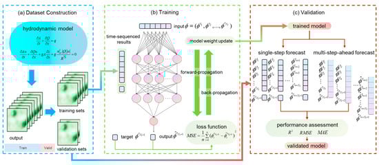
Figure 1.
Workflow of the U-Net-ConvLSTM framework (a) Dataset Construction (b) Training (c) Validation.
2.1.1. Dataset Construction
Hydrodynamic prediction is a typical spatiotemporal prediction problem that requires modeling the spatiotemporal correlation between the independent variables and the predicted dependent variables [28]. The hydrodynamic model’s simulation outputs have both temporal and spatial dimensions. Time was the primary axis in this study, and the first three time steps were used as model inputs to produce the output data in the next time step. Assuming that the current time is , the model input data are then , and the output data are , where is time (s), and is the hydrodynamic indicator (m3/s, m, or m/s) (different values of represent different hydrodynamic indicators, where ), abbreviated as herein. The neural network was trained to establish a generalized mapping relationship between a and b, as shown in the following equation:
The input and output data made up the samples, and the dataset became a collection of samples. In order to speed up model convergence, the dataset was preprocessed before being fed into the model. This ensured that the various data features were kept at the same scale [29]. In this study, the preprocessing was realized by performing min–max normalization [30], which aims to scale the value of each feature within [0,1] with the following equation:
where represents the normalized data. Equation (2) represents the normalization of each feature (hydrodynamic indicator) of the data separately. In the next training–validation process, the dataset was partitioned in the time dimension. Based on Muraina et al.’s research on dataset divisions [31], the percentage of the training set was determined to be 70%, and the percentage of the validation set was determined to be 30%, as shown in Figure 1a. Training is the process of determining the coefficients of the nonlinear relationship , and validation is the process of making predictions using .
2.1.2. Training and Predictive Processes
The training of neural networks is essentially a loss function non-convex optimization problem to solve the minimum value, which is supervised learning, as shown in Figure 1b. It consists of two parts, forward and backward propagation, in which the transformation of input data into output data is realized through forward propagation based on the chain rule, and the output data and the target value are substituted into the loss function to solve the loss. MSE was selected as the loss function to measure the difference between the output data and the target data, as shown in the following equation:
where represents the size of the sample data, and is the time of the predicted data [32]. Back-propagation was performed to update the parameters of the model’s components based on the function values. It started from the output layer, calculated the contribution of each neuron to the value of the loss function layer by layer, and continued to pass the loss value to the upper layer, which was also realized by calculating the gradient through the chain rule [33]. Based on the gradient calculation results, the network parameters were iteratively updated using the gradient descent optimization algorithm to achieve the approximation of the minimum value of the loss function. The training was stopped after determining the model parameters that minimized the loss function and obtained the trained model for validation.
The prediction process was the validation process of the model. The validation of the neural network also used forward propagation, with the difference being that at this point, the model parameters were no longer updated using backpropagation, and only forward propagation was used to calculate the loss in the output data to measure the model accuracy. Two forecasting modes were used to validate the accuracy of the model: one was single-step forecasting, where always uses the data in the validation set and is not updated to make informed long-series forecasts. The second was multi-step-ahead forecasting, where is gradually replaced with predicted data for uninformative long-series prediction, corresponding to the case of missing boundary conditions. The performance evaluation was carried out using the goodness of fit (), root-mean-square error (RMSE), and mean absolute error (MAE). The exact calculational equations will be given in Section 2.4.1.
2.2. Hydrodynamic Models
The Saint-Venant equations were used to describe the hydrodynamic processes in the river reach, and the basic equations are as follows [34].
The continuity equation:
where is the river flow (m3/s), is the length of the channel in the direction of flow (m), is the area of the overwater section (m2), is the time (s), and is the side stream flow (m3/s).
The momentum equation:
where is the flow velocity in the x-direction (m/s), is the acceleration of gravity (m/s2), is the water level (m), is the roughness, and is the hydraulic radius (m).
Equations (4) and (5) were rewritten in a conservation format, and the system of control equations were discretized by the finite volume method using the windward implicit format to obtain the following equations:
where is the generalized form of the conservation equation and stands for or , is the source term, and and are coefficients, and
The detailed calculation of the coefficients will not be repeated here and is described in Zhang et al.’s research [35]. The original nonlinear equations were decomposed into linear equations for each river node, and after uniting the equations for each node, a tridiagonal coefficient matrix was obtained. The hydrodynamic indicators for each node were obtained by solving using the chase method. The validation of the model showed that the relative error between the simulated and validated values of the hydrodynamic indexes was controlled within 5%, which meets the accuracy requirements of a high-fidelity model [27].
2.3. The U-Net-ConvLSTM Framework
This study developed a U-Net-ConvLSTM neural network framework for basin-scale hydrodynamic prediction. Figure 2a shows the structure of the deep U-Net-ConvLSTM neural network, where the 1 × 1 convolutional layer is denoted as to differentiate it from the 3 × 3 convolutional layer, and represents the size of the input data. It is composed of a U-Net network, a ConvLSTM network, and skip connection sections [36,37]. Functionally, it can be divided into an encoding part, decoding part, ConvLSTM part, and skip connection part. The encoding part is used to extract features, the ConvLSTM part is used to learn spatiotemporal features, and the decoding part is used for data upscaling. The skip connection part is set before the pooling layer of the encoding part, which is used for direct communication between the encoding part and the decoding part, so that information lost in the pooling can be passed to the decoding part as much as possible.
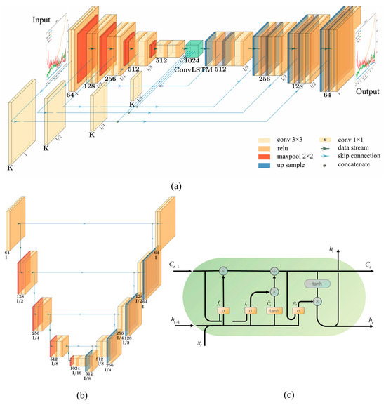
Figure 2.
(a) Architectural diagram of the U-Net-ConvLSTM framework. (b) Architectural diagram of the U-Net framework. (c) Structure of the ConvLSTM cell.
The whole network consists of fourteen network units: nine 3 × 3 convolutional units, a ConvLSTM unit, and four 1 × 1 convolutional units. The 3 × 3 convolutional unit of the coding part consists of two sets of 2D 3 × 3 convolutional and ReLU activation layers and a 2D maximum pooling layer, while the part connected to the ConvLSTM unit is no longer equipped with a maximal pooling layer. The ConvLSTM unit consists of three ConvLSTM layers. The 3 × 3 convolutional unit in the decoding part consists of a 2D up-sampling layer and two sets of 2D convolutional and ReLU activation layers, while a ReLU activation layer was added in the final output part. The 1 × 1 convolutional unit of the skip connection part consists of a 1 × 1 convolutional layer. According to Li et al.’s research and Mu et al.’s research [36,37], the input layer of the encoding part receives batches of temporal data with dimensions (64, 64, 4, 1, batch size) as the input, which is input to the ConvLSTM part after dimensionality reduction to learn complex spatiotemporal features, and after that, it is restored to the previous dimensions after dimensionality upgrading in the decoding part as the output.
2.3.1. U-Net Neural Network Structures
U-Net is essentially a fully convolutional neural network model, which takes its name from the shape of its “U”-shaped architecture, as shown in Figure 2b. The backbone of U-Net is divided into symmetric left and right parts: on the left is the feature extraction network (encoder), where the original input data are down-sampled four times by convolutional–maximum pooling to obtain a feature map at four levels; on the right side is the feature fusion network (decoder), where the feature maps of each layer level are fused with the feature maps obtained after back-convolution through the skip connection part; and the last layer generates predictions by utilizing the acquired features [38]. Its network layer composition was described in the previous section, with the difference being that the connections in the encoding and decoding sections are changed and the skip connection section does not have a convolutional layer. The unique structure allows U-Net to capture pixel-level variations in images [38], which means it is well suited to learning complex spatial features in fluid dynamics data.
2.3.2. ConvLSTM Neural Network Structures
The ConvLSTM network incorporates the advantages of CNN and LSTM networks, which means it can automatically learn hierarchical representations of input data, capturing both low-level spatial details and high-level temporal patterns [39]. The structure of ConvLSTM is similar to LSTM, in which convolutional operations are integrated, as shown in Figure 2c. Its key components are a cell state , input gate , forget gate , and output gate . The cell state is used to transmit information, the input gate is used to receive input data, the forget gate is used to compress the data, and the output gate is used to output the data with the cell state.
The essential equations of ConvLSTM are as follows:
where is the hidden state, and the Hadamard product combines information from different components. Unlike LSTM, the input data of ConvLSTM are tensors in three dimensions and thus can effectively capture spatiotemporal information.
2.4. Predictive Model Accuracy Validation
In order to fully validate the feasibility of the model and evaluate the model performance, the model in Section 2.2 was applied to the hydrodynamic simulation of the middle and lower reaches of the Han River for the period from 2001 to 2020 in order to generate long-time-series spatiotemporal data, and the network was trained and validated using the generated data, applying the network framework to a real case.
Ablation experiments were conducted to comparatively validate the performance of the U-Net-ConvLSTM framework. Based on the CNN, the ConvLSTM part (CNN-ConvLSTM) and the skip connection part (U-Net) were added (U-Net-ConvLSTM), and their performances were evaluated for comparison. Simultaneously, as outlined in Section 2.1.2, both single-step prediction and multi-step-ahead prediction were employed to examine the short-term forecasting ability of the model and the feasibility of long-term forecasting.
2.4.1. Model Evaluation Index
In this study, the model’s performance was assessed using the standard regression parameter , as well as the error indexes RMSE and MAE, with reference to Moriasi‘s research [40]:
1. Goodness of fit ():
2. Root-mean-square error (RMSE):
3. Mean absolute error (MAE):
The model’s performance is considered better when the value approaches 1 and the RMSE and MAE values approach 0.
2.4.2. The Case Study
The Han River, which has a total length of more than 1570 km and is the largest tributary of the Yangtze River, rises in the Qinling Mountains, flows through the provinces of Shaanxi and Hubei, and joins the Yangtze River near Wuhan. The river basin lies between latitudes 30° and 34° north and longitudes 106° and 114° east. The Danjiangkou Reservoir forms the border of the Han River. The middle and lower sections of the river run below it, connecting Zhongxiang and Wuhan in the lower reaches and Danjiangkou to Zhongxiang in the middle [41]. Figure 3 depicts the extent of the Han River’s middle and lower reaches. The middle and lower reaches of the Han River are divided into six sections by five reservoir dams, with a total of 157 cross-sections. The thalweg of the river is shown in Figure S1. The profile of the elevation distribution of the cross-sections is shown in Figures S2 and S3. The hydrodynamic model was constructed based on the spatial locations of these 157 cross-sections and outputs the hydrodynamic information of each cross-section and also serves as the input data for the neural network model. As per the specifications outlined in Section 2.3, the input data for the neural network model underwent a transformation from a size of (157, 4) at time to a size of (64, 64, 4, 1, 1), with any extra space being filled with zeros. Similarly, the data generated at time were resized from (64, 64, 4, 1, 1) to (157, 4) in order to be used in the following data analysis.
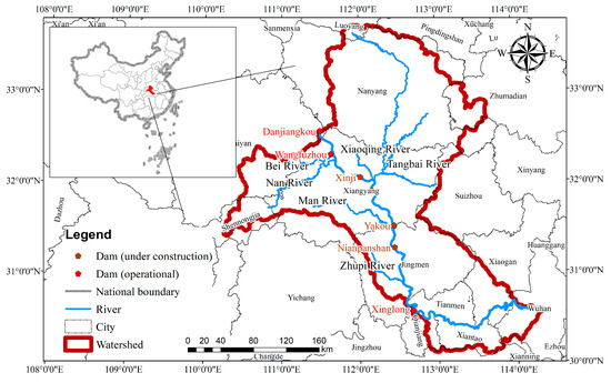
Figure 3.
Overview of study area.
The hydrodynamic conditions of the middle and lower reaches of the Han River are extremely complex under the influence of the construction and operation of graded reservoirs, the withdrawal and recession of water from locks and dams along the river, inter-area inflow and outflow, and downstream top-support. The complex data characteristics brought challenges to the model construction, but with enough sample training, the generalization ability of the model was improved, which was beneficial for the following generalization and application of the model.
The network model was optimally tuned using Adam’s algorithm for parameter weights, the epoch was set to 1000, the initial learning rate was 0.0001, and an early-stop strategy was introduced to terminate the model training. The environment used was a CPU of Intel i7-11850H, a GPU of NVIDIA GTX4080Ti (16 G RAM), and Python 3.10. The number of trainable parameters was 80073690. Mu et al. [37] produced the code for employing U-Net-ConvLSTM for video prediction and also part of the code base for this work. On this basis, the U-Net-ConvLSTM framework was created based on the PyTorch architecture, which is divided into functional modules such as dataset pretreatment, training, prediction, and visualization post-processing.
3. Results and Discussion
In this section, the single-step forecasting results of ConvLSTM-U-Net are first analyzed in comparison with the simulation results of the hydrodynamic model to assess the accuracy and performance of the neural network. The results of the ablation experiments are then parsed to illustrate the advantages offered by the network structure. Finally, the results of the network’s multi-step-ahead forecasting are characterized to test the network’s ability to predict long time series.
3.1. Single-Step Forecasting
U-Net-ConvLSTM was used for the single-step hydrodynamic prediction of 157 sections, 2113 days, and 4 hydrodynamic indicators on the entire validation set and compared with the hydrodynamic model results, as shown in Figure 4. The subplots in Figure 4 reflect the spatial and temporal characteristics of the four hydrodynamic indicators. It can be observed that the hydrodynamic indicators have great heterogeneity in both time and space, with complex changes in characteristics. The U-Net-LSTM prediction results match with the hydrodynamic simulation results, which effectively captures the changing characteristics of the indicators.
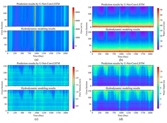
Figure 4.
Single-step prediction performance of U-Net-ConvLSTM on validation set vs. hydrodynamic models: (a) flow, (b) water level, (c) flow velocity, and (d) water depth.
In Figure 4a, it can be seen that there exists a large flooding process at around 900 days, and there is a corresponding trend in Figure 4b–d. U-Net-ConvLSTM predicts this trend well and agrees with the hydrodynamic simulation results in terms of intensity, extent, and duration. Furthermore, the majority of the flow is distributed within the range of 0 to 4000 m3/s. Similarly, the water level is predominantly distributed between 20 and 60 m, while the flow velocities mostly fall within the range of 0 to 1.5 m/s. Additionally, the water depths are primarily distributed between 2 and 10 m. These patterns are effectively captured by the U-Net-ConvLSTM model, and the extrapolated outcomes exhibit a significant level of agreement with the hydrodynamic simulations. In Figure 4c,d, the flow velocity and water depth show high volatility in both time and space, and it can be seen that the model learns the fluctuation characteristics of the data after training and matches the hydrodynamic simulation results in the extreme regions, such as low and high values.
To further evaluate the forecasting accuracy of U-Net-ConvLSTM, the distribution of predicted and target values is described using scatter density plots, as shown in Figure 5. The four hydrodynamic indicators have an above 0.99, the degree of difference is negligible, and there is a strong linear link between the predicted values and target values. The probability density distribution demonstrates that the linear correlation stays strong within the region where the data is most concentrated, suggesting that the model is capable of accurately predicting the majority of the hydrodynamic data characteristics. The slope and intercept of the fitted linear regression line indicate the degree of agreement between the predicted value and the target value. A slope close to one and an intercept close to zero suggest a strong agreement between the predicted and target values. The flow exhibits the smallest slope, 0.9822, among the four indicators, while the intercept exhibits the largest, 17.639. Both values fall within the ideal range, indicating a strong alignment between the predicted and target values. This suggests a high level of accuracy in predicting the four indicators.

Figure 5.
Scatter density plots between predicted and target values: (a) flow, (b) water level, (c) flow velocity, and (d) water depth.
The model evaluation metrics from Section 2.4.1 were used for the prediction performance evaluation, and the results are shown in Table 1. The RMSE and MAE values have a positive connection with the magnitude of the indicator, consistently remaining at a low level. This suggests that the model possesses a strong capability to accurately forecast future time-step results.

Table 1.
Evaluation results of single-step forecasting for U-Net-ConvLSTM.
Regarding computational efficiency, it is noteworthy that the GPU time required for a single-step prediction using U-Net-ConvLSTM is 0.03 s, while the CPU time for a single-step prediction using the hydrodynamic model is 0.07 s. The utilization of U-Net-ConvLSTM efficiently decreases the hydrodynamic prediction time cost, as evidenced by a 62.08% reduction in the computational time for the neural network. Furthermore, the network training process takes approximately 12 h. When compared with the costly expenses associated with developing hydrodynamic models, a neural network model offers a more affordable and efficient alternative for predicting hydrodynamic outcomes, requiring only minimal training.
3.2. Ablation Experiments
The CNN-ConvLSTM network, U-Net network, and U-Net-ConvLSTM network are employed for training and validation in this section, respectively. Their performances on the training sets and validation sets during training are documented to comparatively assess the impacts of incorporating the ConvLSTM part and the skip connection part on the predictive capabilities of the models.
The performances of the three networks during training are illustrated in Figure 6. It examines how the RMSE of the single-iteration prediction results varies with the number of iterations for different network architectures. Overall, U-Net-ConvLSTM has the lowest RMSE on both the training sets and validation sets, U-Net has a slightly higher RMSE than U-Net-ConvLSTM, and CNN-ConvLSTM is comparatively poor in predictive performance. The RMSE fluctuation range of U-Net is similar to that of U-Net-ConvLSTM. However, as depicted in the inset in Figure 6, toward the end of the training, the RMSE of U-Net surpasses that of U-Net-ConvLSTM, providing evidence for the superiority of the U-Net-ConvLSTM framework.
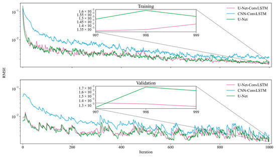
Figure 6.
Trends of RMSEs of the three frameworks with the number of iterations on the training and validation sets during the training period.
The predictive accuracies of the three network frameworks on the training and validation sets after completing the training process are displayed in Table 2. The inclusion of the skip connection part in U-Net-ConvLSTM resulted in a significant average reduction of 33.34% in the RMSE of the predictors compared with CNN-ConvLSTM. Similarly, the addition of the ConvLSTM part in U-Net led to an average drop of 1.68% in the RMSE of the predictors. The inclusion of either the skip connection component or the ConvLSTM component is observed to have a beneficial effect on the accuracy of predictions. The model’s performance is further enhanced when both modules are used.
Table 2.
Evaluation results of three frameworks.
3.3. Multi-Step-Ahead Forecasting
The prediction accuracy of the model from 1 day to 5 days was explored on the validation set to assess the ability of the model to create multi-step-ahead forecasts, and the RMSE, MAE, and of the forecasting results for the four hydrodynamic metrics are presented in Figure 7. As time progresses, the prediction accuracy continues to diminish, and errors accumulate, with the average RMSE of the four measures increasing to 4.3 times that on day 1 on day 5, and the average MAE increasing to 5.1 times that on day 1 on day 5. In general, the is consistently maintained at a high level, decreasing by approximately 8% on average for the entire duration. The minimal value of is above 0.7, indicating that the model’s multi-step-ahead forecasting are still fairly dependable [40].
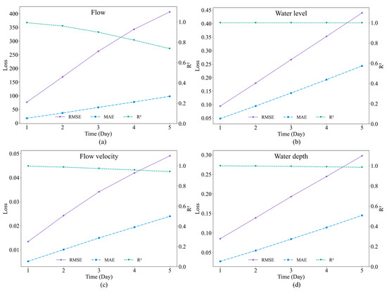
Figure 7.
Trend of model evaluation metrics of U-Net-ConvLSTM with prediction span in multi-step-ahead forecasting mode: (a) flow, (b) water level, (c) flow velocity, and (d) water depth.
Furthermore, as illustrated in Figure S4, U-Net-ConvLSTM demonstrates superior performance compared with U-Net and CNN-ConvLSTM. This is due to the fact that the accumulation of little errors can lead to significant variations in the outcomes of subsequent multi-step predictions. Consequently, U-Net-ConvLSTM is the more favorable option when subjected to thorough evaluation. The time required for multi-step-ahead prediction using the model is similar to that for single-step prediction. U-Net-ConvLSTM demonstrates the ability to forecast hydrodynamic outcomes with high accuracy over an extended duration in a relatively short timeframe. Furthermore, it can predict future hydrodynamic circumstances even when boundary conditions are not provided. This effectively addresses the constraints of conventional hydrodynamic mechanism models and improves the computing efficiency of large-scale hydrodynamic simulation and prediction.
Accurate and complete historical datasets are the primary guarantee for the prediction accuracy of neural networks, but real data in practical settings generally encounter challenges such as missing data, low quality, and multi-source heterogeneity, which inhibit the application of neural networks [8]. The data obtained from hydrodynamic modeling effectively address this limitation and offer numerous high-quality datasets for U-Net-ConvLSTM. In addition, the predictive capability of U-Net-ConvLSTM diminishes as the prediction timeframe increases. To maintain prediction accuracy, data assimilation with hydrodynamic simulation results is considered as the next research focus [39]. The deep integration of deep learning with hydrodynamic modeling effectively compensates for the limitations of both in hydrodynamic prediction.
4. Conclusions
This paper constructed a deep learning framework called U-Net-ConvLSTM based on the hydrodynamic model, in which the hydrodynamic model offers precise and comprehensive spatiotemporal datasets of hydrodynamic indicators for U-Net-ConvLSTM. On the other hand, U-Net-ConvLSTM addresses the computational challenges arising from large computational scales, long prediction spans, and boundary uncertainties by establishing a connection between historical and future data. The integration of both components allows the model to attain precise and effective hydrodynamic forecasts in a large-scale basin, even when boundary conditions are not available. The main research findings are as follows:
- (1)
- U-Net-ConvLSTM demonstrated excellent predictive performance on a long-series hydrodynamic dataset generated by a high-fidelity mechanistic model. It achieved an overall value above 0.99 and closely matched the results of the CFD simulation. Additionally, both the RMSE and MAE were maintained at a low level. U-Net-ConvLSTM decreased the time taken for single-step prediction by 62.08% when compared with conventional mechanistic models. These findings suggest that the proposed framework is stable and capable of accurately and efficiently predicting future time-step results.
- (2)
- When compared with CNN-ConvLSTM and U-Net, U-Net-ConvLSTM proved its usefulness by reducing the RMSE values used to calibrate the prediction error on the entire dataset by 33.34% and 1.68% after incorporating the skip connection part and the ConvLSTM part, respectively.
- (3)
- The model’s prediction horizon expanded from 1 to 5 days, resulting in a loss of just 8% in the value. Despite this decline, the value remained above 0.7, indicating a high level of accuracy. This demonstrates the model’s robustness and reliability in making multi-step-ahead predictions and also exemplifies the usability of the model in the case of lacking boundary conditions.
U-Net-ConvLSTM is capable of capturing the intricate nonlinear characteristics of large-scale hydrodynamic spatiotemporal data. This enables more precise and efficient hydrodynamic predictions while also facilitating the high-performance computing of basin-scale hydrodynamics.
Supplementary Materials
The following supporting information can be downloaded at https://www.mdpi.com/article/10.3390/w16050625/s1. Figure S1: The thalweg of river in the middle and lower reaches of the Han River; Figure S2: Schematic distribution of channel section elevations in the middle and lower reaches of the Han River; Figure S3: Elevation dispersion in certain cross-sections of the middle and lower stretches of the Hanjiang River; Figure S4: Trend of RMSE of U-Net-ConvLSTM, CNN-ConvLSTM, and U-Net with prediction span in multi-step-ahead forecasting mode.
Author Contributions
Conceptualization, W.Z.; methodology, A.L., W.Z. and X.Z.; formal analysis, A.L.; investigation, A.L. and F.Z.; data curation, A.L.; writing—original draft preparation, A.L.; writing—review and editing, W.Z., X.Z., G.C., X.L., A.J. and H.P.; visualization, A.L.; supervision, W.Z., X.Z. and G.C.; funding acquisition, W.Z. All authors have read and agreed to the published version of the manuscript.
Funding
This work was supported by the National Natural Science Foundation of China (grant number 41877531) and the National Key Research and Development Program of China (grant numbers 2017YFC1502500 and 2016YFC0402201).
Data Availability Statement
The data presented in this study are available upon request from the corresponding authors. The data are not publicly available due to privacy.
Conflicts of Interest
The authors declare no conflicts of interest.
Abbreviations
| R2 | Goodness of fit |
| CFD | Computational fluid dynamics |
| LSTM | Long short-term memory |
| CNN | Convolutional neural network |
| ConvLSTM | Convolutional LSTM |
| MSE | Mean square error |
| RMSE | Root-mean-square error |
| MAE | Mean absolute error |
| Nomenclature | |
| The flow velocity in the x-direction (m/s) | |
| The river flow (m3/s) | |
| The length of the channel along the direction of flow (m) | |
| Water level (m) | |
| Time (s) | |
| Hydrodynamic indicator: k = 1—flow (m3/s) k = 2—water level (m) k = 3—flow velocity (m/s) k = 4—water depth (m) | |
| ^ | Simulated values: |
| Markers for distinguishing between 1 × 1 convolutional layers and 3×3 convolutional layers | |
| The size of the input data | |
| The area of the overwater section (m2) | |
| The side stream flow (m3/s) | |
| The acceleration of gravity (m/s2) | |
| The roughness | |
| The hydraulic radius (m) | |
| The coefficients [10] | |
| Source term | |
| Cell state | |
| Input gate | |
| Forget gate | |
| Output gate | |
| The hidden state | |
| The Hadamard product | |
References
- Ibrahim, A.; Meguid, M.A. CFD-DEM simulation of sand erosion into defective gravity pipes under constant groundwater table. Tunn. Undergr. Sp. Tech. 2023, 131, 104823. [Google Scholar] [CrossRef]
- Loli, M.; Mitoulis, S.A.; Tsatsis, A.; Manousakis, J.; Kourkoulis, R.; Zekkos, D. Flood characterization based on forensic analysis of bridge collapse using UAV reconnaissance and CFD simulations. Sci. Total Environ. 2022, 822, 153661. [Google Scholar] [CrossRef]
- Xie, D.; Zou, Q.; Mignone, A.; MacRae, J.D. Coastal flooding from wave overtopping and sea level rise adaptation in the northeastern USA. Coast. Eng. 2019, 150, 39–58. [Google Scholar] [CrossRef]
- Liu, M.; Zhang, Z. Smoothed particle hydrodynamics (SPH) for modeling fluid-structure interactions. Sci. China Phys. Mech. Astron. 2019, 62, 984701. [Google Scholar] [CrossRef]
- Sukhinov, A.I.; Chistyakov, A.E.; Alekseenko, E.V. Numerical realization of the three-dimensional model of hydrodynamics for shallow water basins on a high-performance system. Math. Models Comput. Simul. 2011, 3, 562–574. [Google Scholar] [CrossRef]
- Chen, G.; Zhang, W.; Liu, X.; Peng, H.; Zhou, F.; Wang, H.; Ke, Q.; Xiao, B. Development and application of a multi-centre cloud platform architecture for water environment management. J. Environ. Manag. 2023, 344, 118670. [Google Scholar] [CrossRef] [PubMed]
- Xie, M.; Shan, K.; Zeng, S.; Wang, L.; Gong, Z.; Wu, X.; Yang, B.; Shang, M. Combined Physical Process and Deep Learning for Daily Water Level Simulations across Multiple Sites in the Three Gorges Reservoir, China. Water 2023, 15, 3191. [Google Scholar] [CrossRef]
- Shen, C.; Appling, A.P.; Gentine, P.; Bandai, T.; Gupta, H.; Tartakovsky, A.; Baity-Jesi, M.; Fenicia, F.; Kifer, D.; Li, L.; et al. Differentiable modelling to unify machine learning and physical models for geosciences. Nat. Rev. Earth Environ. 2023, 4, 552–567. [Google Scholar] [CrossRef]
- Xue, P.; Wagh, A.; Ma, G.; Wang, Y.; Yang, Y.; Liu, T.; Huang, C. Integrating Deep Learning and Hydrodynamic Modeling to Improve the Great Lakes Forecast. Remote Sens. 2022, 14, 2640. [Google Scholar] [CrossRef]
- Ladwig, R.; Daw, A.; Albright, E.A.; Buelo, C.; Karpatne, A.; Meyer, M.F.; Neog, A.; Hanson, P.C.; Dugan, H.A. Modular Compositional Learning Improves 1D Hydrodynamic Lake Model Performance by Merging Process-Based Modeling with Deep Learning. J. Adv. Model. Earth Syst. 2024, 16, e2023MS003953. [Google Scholar] [CrossRef]
- Li, G.; Zhu, H.; Jian, H.; Zha, W.; Wang, J.; Shu, Z.; Yao, S.; Han, H. A combined hydrodynamic model and deep learning method to predict water level in ungauged rivers. J. Hydrol. 2023, 625, 130025. [Google Scholar] [CrossRef]
- Wang, Y.; Yang, Y.; Chen, X.; Engel, B.A.; Zhang, W. The moving confluence route technology with WAD scheme for 3D hydrodynamic simulation in high altitude inland waters. J. Hydrol. 2018, 559, 411–427. [Google Scholar] [CrossRef]
- Ajami, N.K.; Duan, Q.; Sorooshian, S. An integrated hydrologic Bayesian multimodel combination framework: Confronting input, parameter, and model structural uncertainty in hydrologic prediction. Water Resour. Res. 2007, 43, W01403. [Google Scholar] [CrossRef]
- LeCun, Y.; Bengio, Y.; Hinton, G. Deep learning. Nature 2015, 521, 436–444. [Google Scholar] [CrossRef]
- Hu, R.; Fang, F.; Pain, C.C.; Navon, I.M. Rapid spatio-temporal flood prediction and uncertainty quantification using a deep learning method. J. Hydrol. 2019, 575, 911–920. [Google Scholar] [CrossRef]
- Liu, Y.; Yang, Y.; Chin, R.J.; Wang, C.; Wang, C. Long Short-Term Memory (LSTM) Based Model for Flood Forecasting in Xiangjiang River. Ksce J. Civ. Eng. 2023, 27, 5030–5040. [Google Scholar] [CrossRef]
- Li, P.; Zhang, J.; Krebs, P. Prediction of Flow Based on a CNN-LSTM Combined Deep Learning Approach. Water 2022, 14, 993. [Google Scholar] [CrossRef]
- Chen, J.; Li, Y.; Zhang, S. Fast Prediction of Urban Flooding Water Depth Based on CNN-LSTM. Water 2023, 15, 1397. [Google Scholar] [CrossRef]
- Zhang, J.; Wang, Z.; Bai, L.; Song, G.; Tao, J.; Chen, L. Deforestation Detection Based on U-Net and LSTM in Optical Satellite Remote Sensing Images. In Proceedings of the 2021 IEEE International Geoscience and Remote Sensing Symposium IGARSS, Brussels, Belgium, 11–16 July 2021; pp. 3753–3756. [Google Scholar]
- Yin, L.; Wang, L.; Li, T.; Lu, S.; Tian, J.; Yin, Z.; Li, X.; Zheng, W. U-Net-LSTM: Time Series-Enhanced Lake Boundary Prediction Model. Land 2023, 12, 1859. [Google Scholar] [CrossRef]
- Hou, Y.; Li, H.; Chen, H.; Wei, W.; Wang, J.; Huang, Y. A novel deep U-Net-LSTM framework for time-sequenced hydrodynamics prediction of the SUBOFF AFF-8. Eng. Appl. Comp. Fluid 2022, 16, 630–645. [Google Scholar] [CrossRef]
- Portal-Porras, K.; Fernandez-Gamiz, U.; Zulueta, E.; Irigaray, O.; Garcia-Fernandez, R. Hybrid LSTM+CNN architecture for unsteady flow prediction. Mater. Today Commun. 2023, 35, 106281. [Google Scholar] [CrossRef]
- Shi, X.; Chen, Z.; Wang, H.; Yeung, D.; Wong, W.; Woo, W. Convolutional LSTM network: A machine learning approach for precipitation nowcasting. Adv. Neural Inf. Process. Syst. 2015, 28, 802–810. [Google Scholar]
- Lin, Z.; Li, M.; Zheng, Z.; Cheng, Y.; Yuan, C. Self-attention convlstm for spatiotemporal prediction. AAAI 2020, 34, 11531–11538. [Google Scholar] [CrossRef]
- Lai, X.; Jiang, J.; Liang, Q.; Huang, Q. Large-scale hydrodynamic modeling of the middle Yangtze River Basin with complex river–lake interactions. J. Hydrol. 2013, 492, 228–243. [Google Scholar] [CrossRef]
- Sheikholeslami, S.; Meister, M.; Wang, T.; Payberah, A.H.; Vlassov, V.; Dowling, J. AutoAblation: Automated Parallel Ablation Studies for Deep Learning. In EuroMLSys ’21; Association for Computing Machinery: New York, NY, USA, 2021; pp. 55–61. [Google Scholar]
- Wang, Y.; Zhang, W.; Zhao, Y.; Peng, H.; Shi, Y. Modelling water quality and quantity with the influence of inter-basin water diversion projects and cascade reservoirs in the Middle-lower Hanjiang River. J. Hydrol. 2016, 541, 1348–1362. [Google Scholar] [CrossRef]
- Xu, L.; Chen, N.; Chen, Z.; Zhang, C.; Yu, H. Spatiotemporal forecasting in earth system science: Methods, uncertainties, predictability and future directions. Earth-Sci. Rev. 2021, 222, 103828. [Google Scholar] [CrossRef]
- Sun, J.; Cao, X.; Liang, H.; Huang, W.; Chen, Z.; Li, Z. New interpretations of normalization methods in deep learning. arXiv 2020, arXiv:2006.09104. [Google Scholar] [CrossRef]
- Eesa, A.S.; Arabo, W.K. A Normalization Methods for Backpropagation: A Comparative Study. Sci. J. Univ. Zakho 2017, 5, 319–323. [Google Scholar] [CrossRef]
- Muraina, I. Ideal Dataset Splitting Ratios in Machine Learning Algorithms: General Concerns for Data Scientists and Data Analysts. In 7th International Mardin Artuklu Scientific Researches Conference; Mardin Artuklu: Mardin, Turkey, 2022. [Google Scholar]
- Cheng, M.; Fang, F.; Navon, I.M.; Zheng, J.; Zhu, J.; Pain, C. Assessing uncertainty and heterogeneity in machine learning-based spatiotemporal ozone prediction in Beijing-Tianjin- Hebei region in China. Sci. Total Environ. 2023, 881, 163146. [Google Scholar] [CrossRef] [PubMed]
- Cheng, M.; Fang, F.; Pain, C.C.; Navon, I.M. Data-driven modelling of nonlinear spatio-temporal fluid flows using a deep convolutional generative adversarial network. Comput. Method. Appl. Mech. Eng. 2020, 365, 113000. [Google Scholar] [CrossRef]
- Zhang, W.; Wang, Y.; Peng, H.; Li, Y.; Tang, J.; Wu, K.B. A Coupled Water Quantity–Quality Model for Water Allocation Analysis. Water Resour. Manag. 2010, 24, 485–511. [Google Scholar] [CrossRef]
- Lu, W.Z.; Zhang, W.S.; Cui, C.Z.; Leung, A.Y.T. A numerical analysis of free-surface flow in curved open channel with velocity–pressure-free-surface correction. Comput. Mech. 2004, 33, 215–224. [Google Scholar] [CrossRef]
- Li, Y.; Cai, Y.; Liu, J.; Lang, S.; Zhang, X. Spatio-Temporal Unity Networking for Video Anomaly Detection. IEEE Access 2019, 7, 172425–172432. [Google Scholar] [CrossRef]
- R_Unet. 2015. Available online: https://github.com/Michael-MuChienHsu/R_Unet (accessed on 22 December 2020).
- Siddique, N.; Paheding, S.; Elkin, C.P.; Devabhaktuni, V. U-Net and Its Variants for Medical Image Segmentation: A Review of Theory and Applications. IEEE Access 2021, 9, 82031–82057. [Google Scholar] [CrossRef]
- Cheng, M.; Fang, F.; Navon, I.M.; Pain, C. Ensemble Kalman filter for GAN-ConvLSTM based long lead-time forecasting. J. Comput. Sci. 2023, 69, 102024. [Google Scholar] [CrossRef]
- Moriasi, D.; Arnold, J.; Van Liew, M.; Bingner, R.; Harmel, R.D.; Veith, T. Model Evaluation Guidelines for Systematic Quantification of Accuracy in Watershed Simulations. Trans. ASABE 2007, 50, 885–900. [Google Scholar] [CrossRef]
- Zhang, X.; Yang, H.; Zhang, W.; Fenicia, F.; Peng, H.; Xu, G. Hydrologic impacts of cascading reservoirs in the middle and lower Hanjiang River basin under climate variability and land use change. J. Hydrol. Reg. Stud. 2022, 44, 101253. [Google Scholar] [CrossRef]
Disclaimer/Publisher’s Note: The statements, opinions and data contained in all publications are solely those of the individual author(s) and contributor(s) and not of MDPI and/or the editor(s). MDPI and/or the editor(s) disclaim responsibility for any injury to people or property resulting from any ideas, methods, instructions or products referred to in the content. |
© 2024 by the authors. Licensee MDPI, Basel, Switzerland. This article is an open access article distributed under the terms and conditions of the Creative Commons Attribution (CC BY) license (https://creativecommons.org/licenses/by/4.0/).