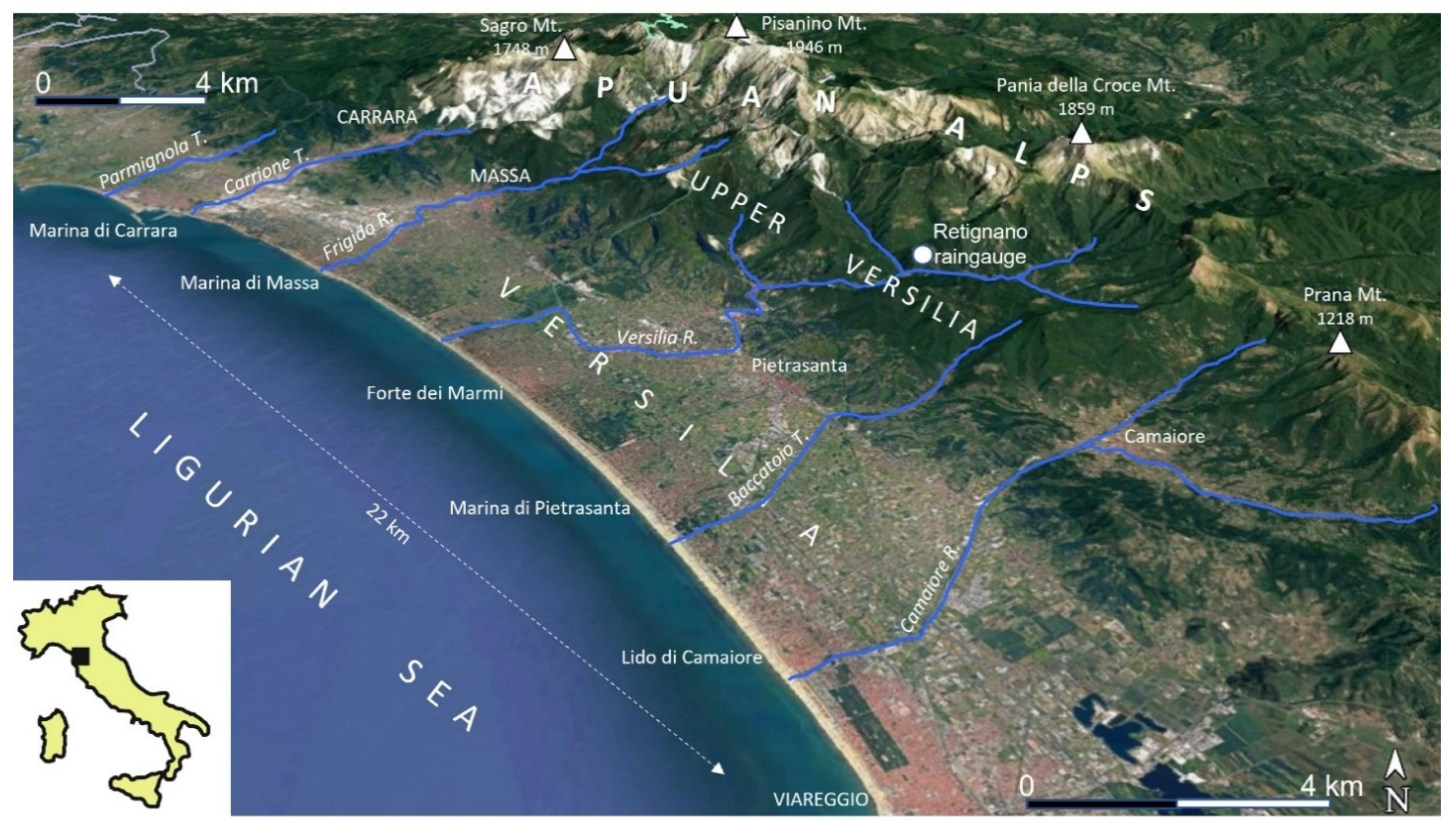
Figure 1.
Location map and main morphological features of the Apuan Alps (white circle: Retignano raingauge; white triangles: main mountains and relative altitude in m a.s.l.; blue lines: main rivers and torrents. Being a 3D-perspective, the upper and lower scale are showed, along with the distance between two towns, as scale references (3D-perspective by Google Maps).
Figure 2.
Shallow landslides activated by the rainstorm of 19 June 1996. The upper left inset shows the main village destroyed by the debris torrents, causing 13 deaths (adapted with permission from [
14]. 2004, Elsevier).
Figure 2.
Shallow landslides activated by the rainstorm of 19 June 1996. The upper left inset shows the main village destroyed by the debris torrents, causing 13 deaths (adapted with permission from [
14]. 2004, Elsevier).
Figure 3.
Rainfall thresholds obtained using LR method for the 1975–2002 period and corresponding to different landslide probability (5–90%). Blue squares: events that did not trigger landslides (NSLE); red lozenges: events that triggered landslides (SLE).
Figure 3.
Rainfall thresholds obtained using LR method for the 1975–2002 period and corresponding to different landslide probability (5–90%). Blue squares: events that did not trigger landslides (NSLE); red lozenges: events that triggered landslides (SLE).
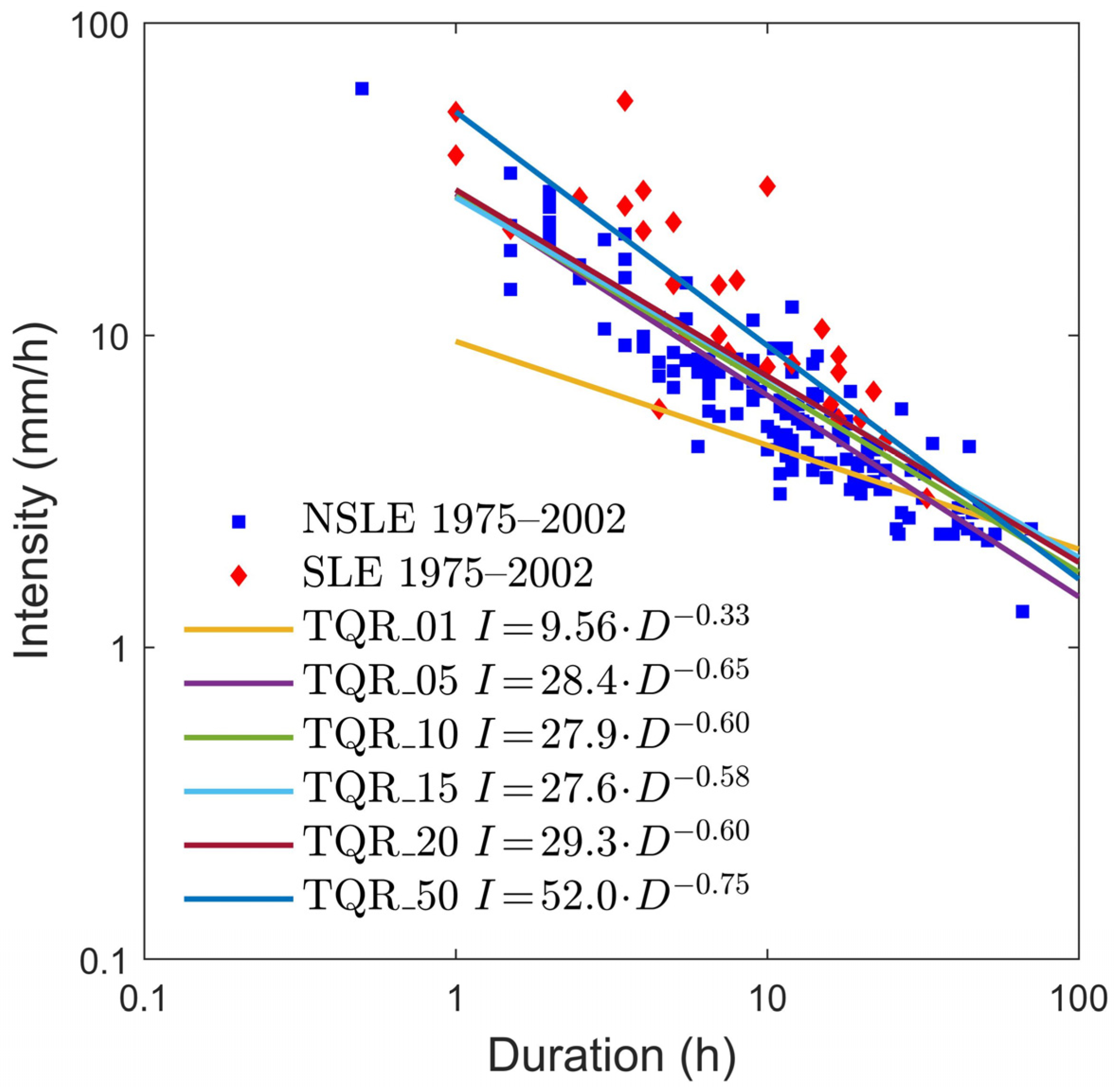
Figure 4.
Rainfall thresholds obtained using QR method for the 1975–2002 period and corresponding to different landslide probability (1–50%). Blue squares: events that did not trigger landslides (NSLE); red lozenges: events that triggered landslides (SLE).
Figure 4.
Rainfall thresholds obtained using QR method for the 1975–2002 period and corresponding to different landslide probability (1–50%). Blue squares: events that did not trigger landslides (NSLE); red lozenges: events that triggered landslides (SLE).
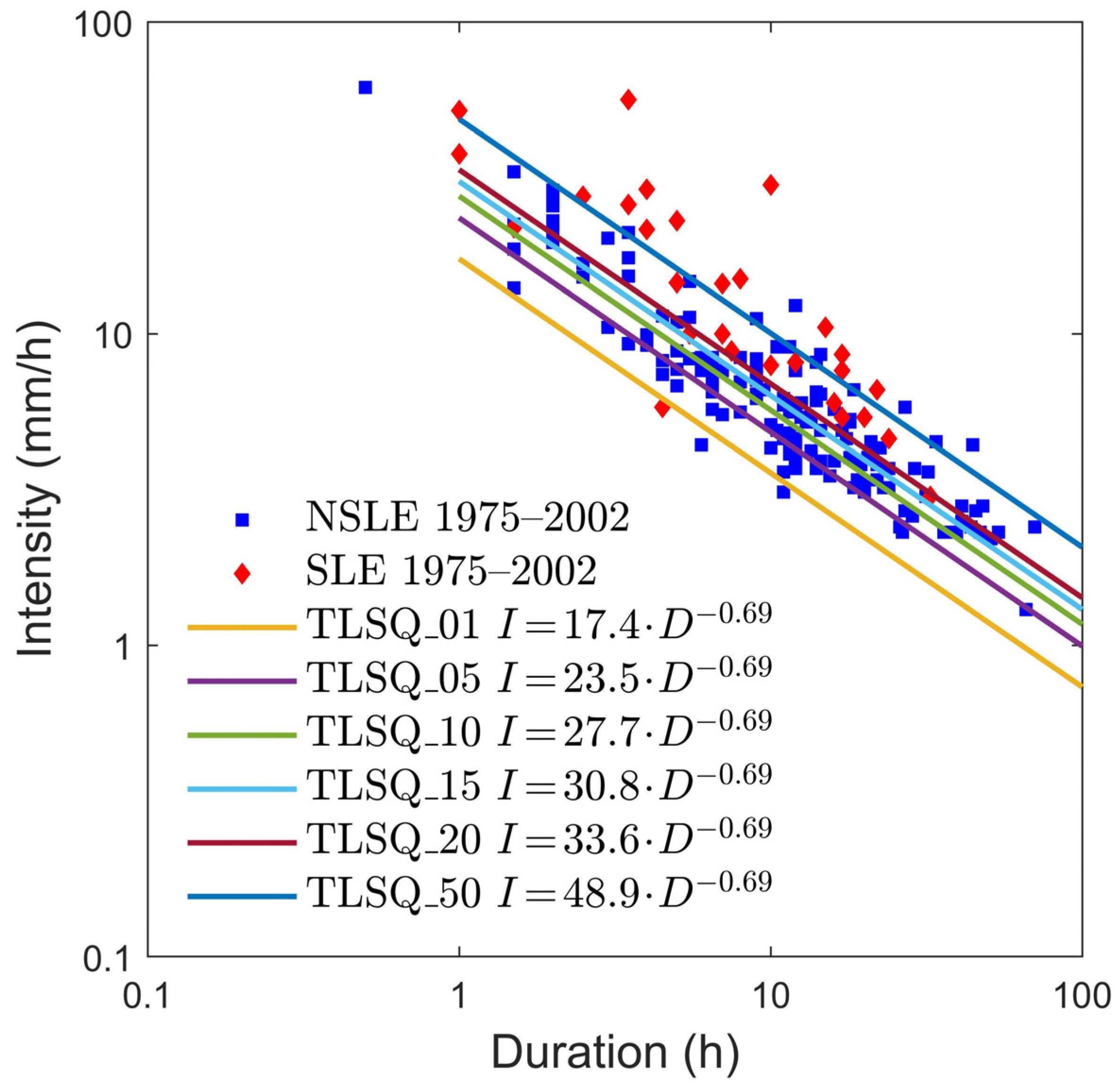
Figure 5.
Rainfall thresholds obtained using the LSQ method for the 1975–2002 period and corresponding to different landslide probabilities (1–50%). Blue squares: events that did not trigger landslides (NSLE); red lozenges: events that triggered landslides (SLE).
Figure 5.
Rainfall thresholds obtained using the LSQ method for the 1975–2002 period and corresponding to different landslide probabilities (1–50%). Blue squares: events that did not trigger landslides (NSLE); red lozenges: events that triggered landslides (SLE).
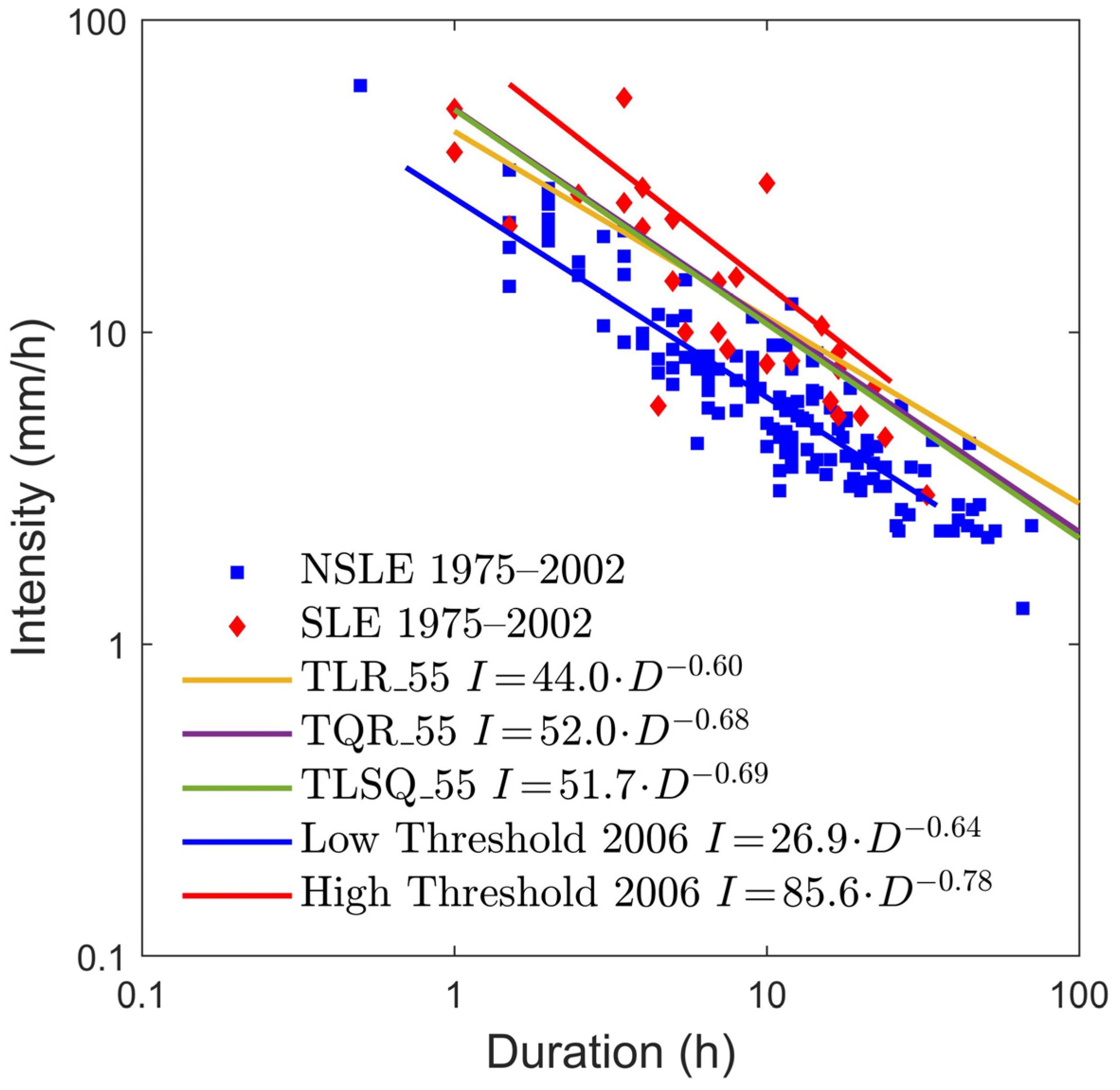
Figure 6.
Comparison among the upper and lower rainfall thresholds of [
27] (red and blue lines, respectively) and those obtained by the three statistical methods (yellow, green, violet lines) considering the maximum efficiency related to 1975–2002 period. Blue squares: events that did not trigger landslides (NSLE); red lozenges: events that triggered landslides (SLE).
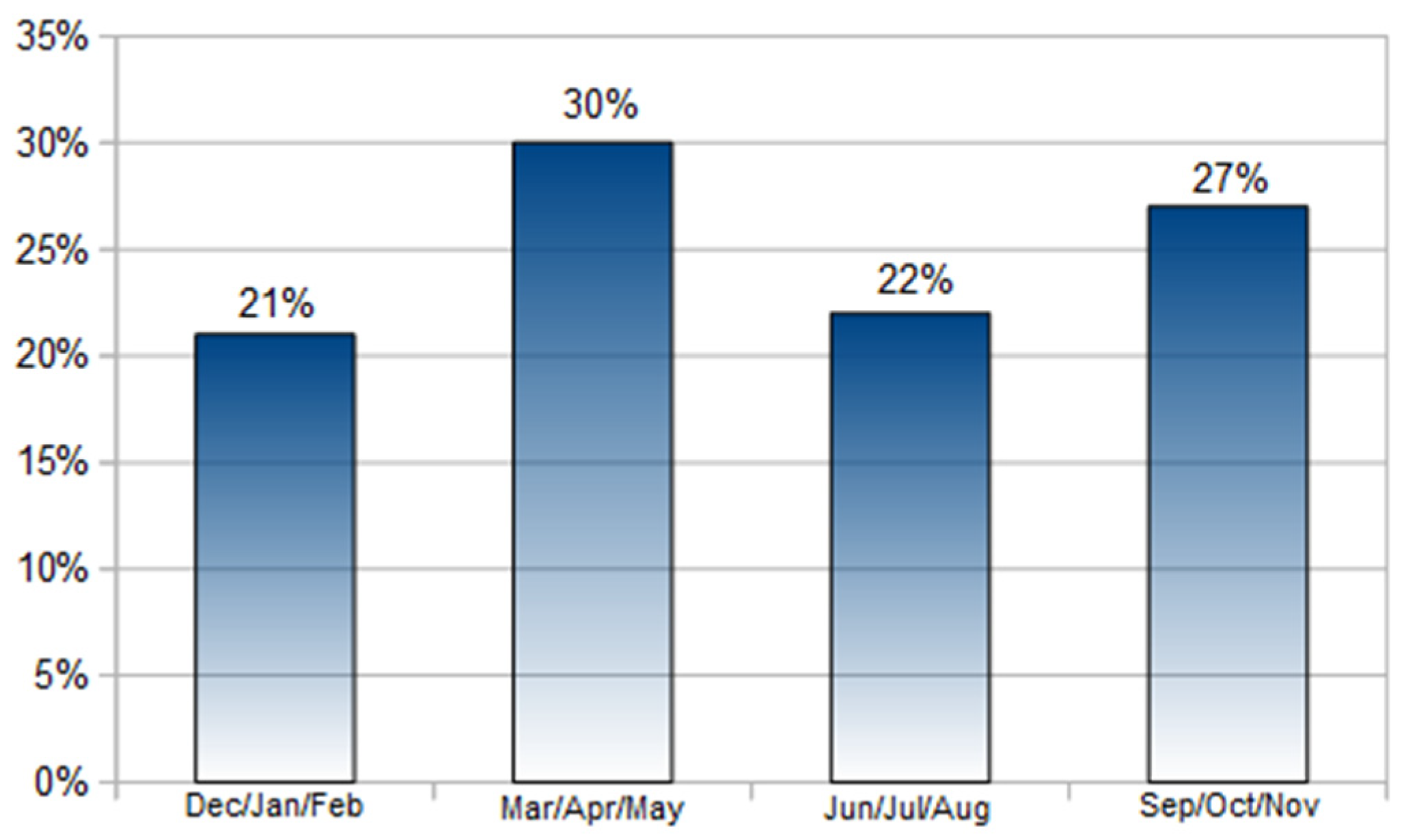
Figure 7.
Distribution of main rainfall events that occurred in the southern Apuan Alps from 2008 to 2016 in relation to season.
Figure 7.
Distribution of main rainfall events that occurred in the southern Apuan Alps from 2008 to 2016 in relation to season.
Figure 8.
Distribution of rainfall events inducing shallow landslides (SLE) in the southern Apuan Alps from 2008 to 2016 in relation to season.
Figure 8.
Distribution of rainfall events inducing shallow landslides (SLE) in the southern Apuan Alps from 2008 to 2016 in relation to season.
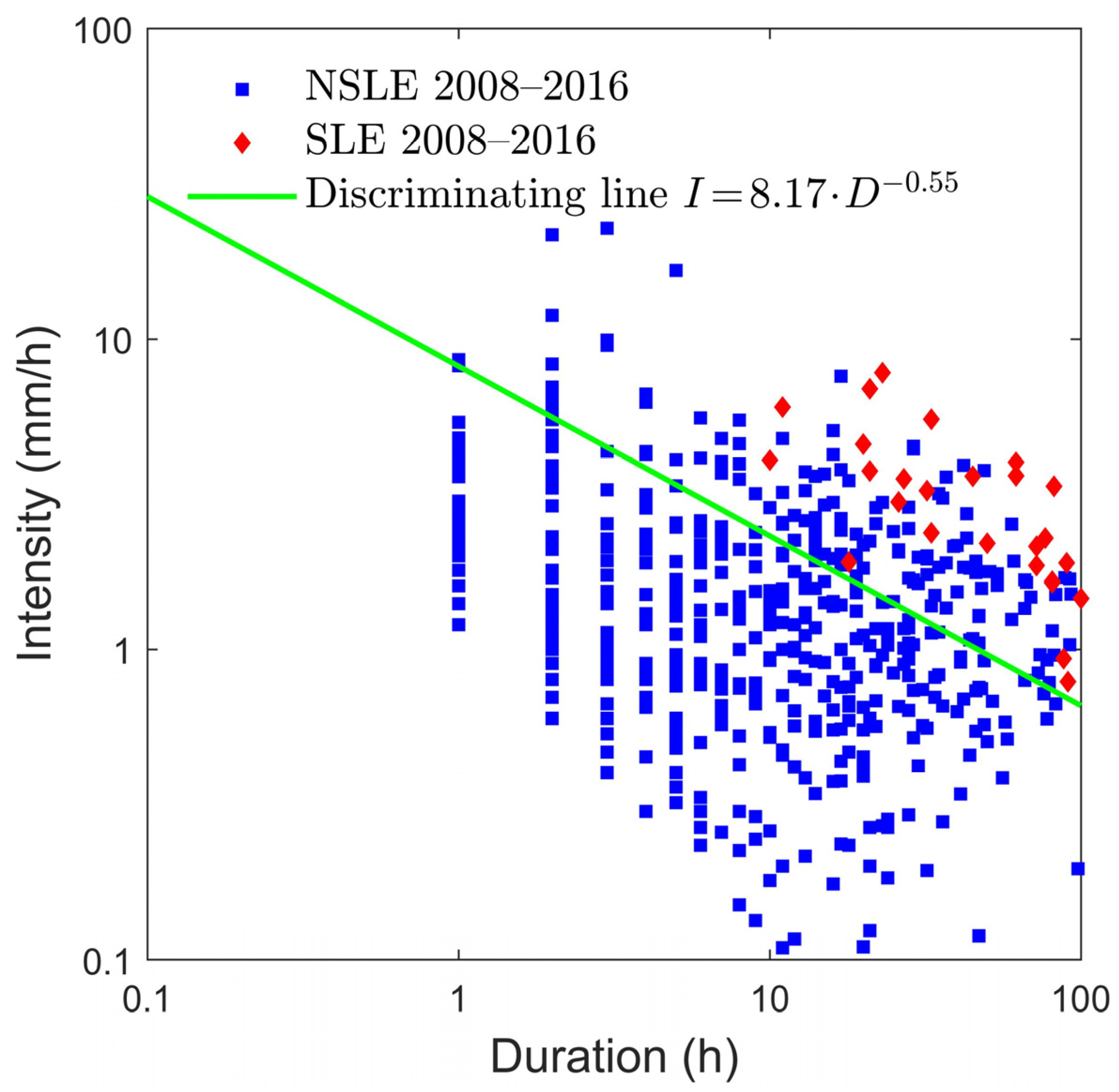
Figure 9.
ID log-log plot of rainfall events SLEs and NSLEs of the 2008–2016 period reconstructed using the algorithm [
52]. Green line separates events considered significant (above the green line) from events that instead cause a bias in the results (below the green line) due to an increase of the number of TN in the contingency tables and, therefore, a considerable increase of the efficiency values (Ef). Blue squares: events that did not trigger landslides (NSLE); red lozenges: events that triggered landslides (SLE).
Figure 10.
ID log-log plot of rainfall events SLEs and NSLEs of the 2008–2016 period located above the discriminating line shown in
Figure 9. Blue squares: events that did not trigger landslides (NSLE); red lozenges: events that triggered landslides (SLE).
Figure 10.
ID log-log plot of rainfall events SLEs and NSLEs of the 2008–2016 period located above the discriminating line shown in
Figure 9. Blue squares: events that did not trigger landslides (NSLE); red lozenges: events that triggered landslides (SLE).
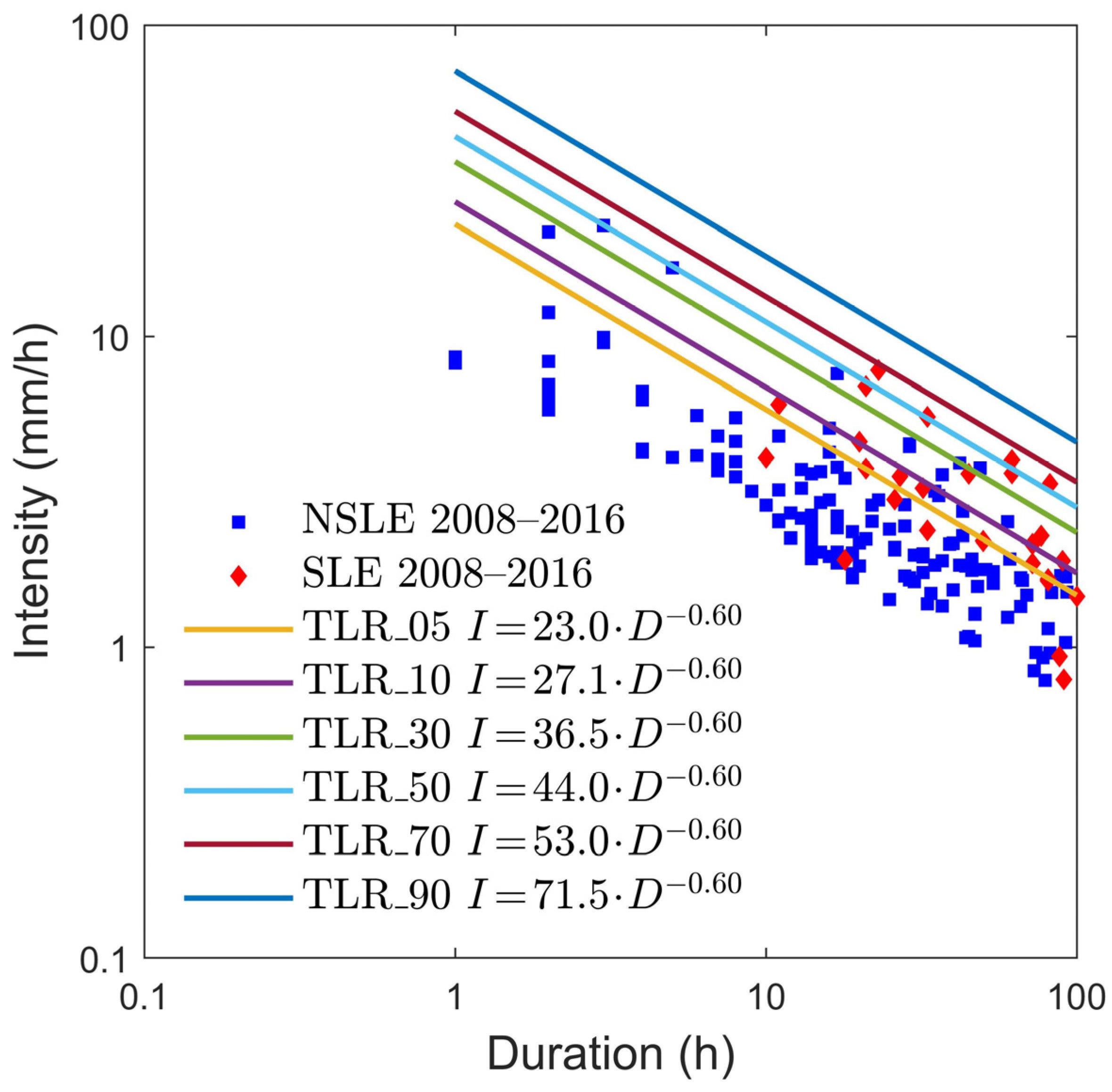
Figure 11.
Rainfall thresholds obtained by using the LR method for the 2008–2016 period and corresponding to different landslide probabilities (5–90%). Blue squares: events that did not trigger landslides (NSLE); red lozenges: events that triggered landslides (SLE).
Figure 11.
Rainfall thresholds obtained by using the LR method for the 2008–2016 period and corresponding to different landslide probabilities (5–90%). Blue squares: events that did not trigger landslides (NSLE); red lozenges: events that triggered landslides (SLE).
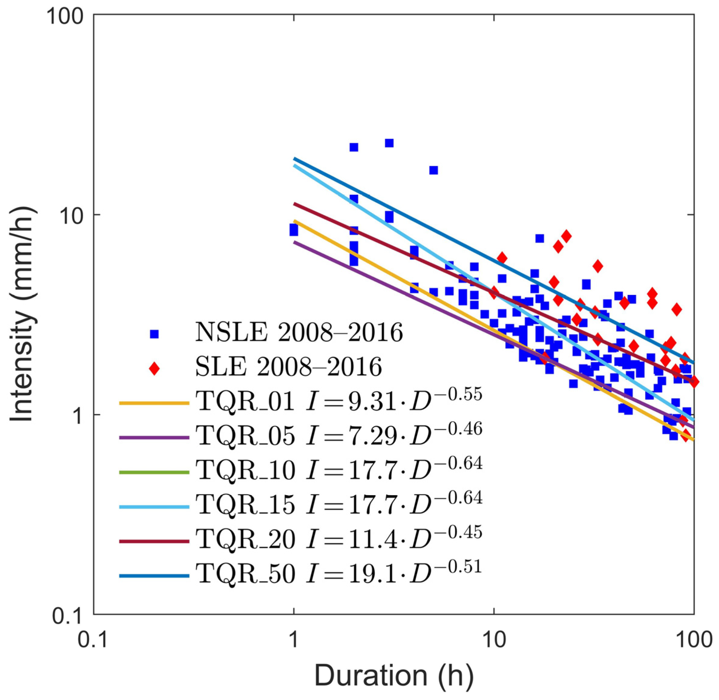
Figure 12.
Rainfall thresholds obtained using the QR method for the 2008–2016 period and corresponding to different landslide probabilities (1–50%). The TQR_10 and TQR_15 lines are perfectly superimposed (only the light blue one is shown). Blue squares: events that did not trigger landslides (NSLE); red lozenges: events that triggered landslides (SLE).
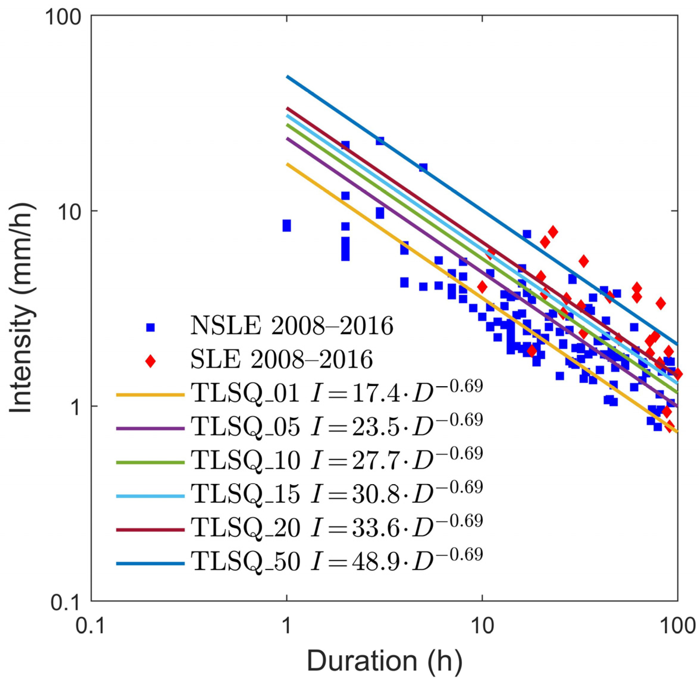
Figure 13.
Rainfall thresholds obtained using the LSQ method for the 2008–2016 period and corresponding to different landslide probabilities (1–50%). Blue squares: events that did not triggered landslides (NSLE); red lozenges: events that triggered landslides (SLE).
Figure 13.
Rainfall thresholds obtained using the LSQ method for the 2008–2016 period and corresponding to different landslide probabilities (1–50%). Blue squares: events that did not triggered landslides (NSLE); red lozenges: events that triggered landslides (SLE).
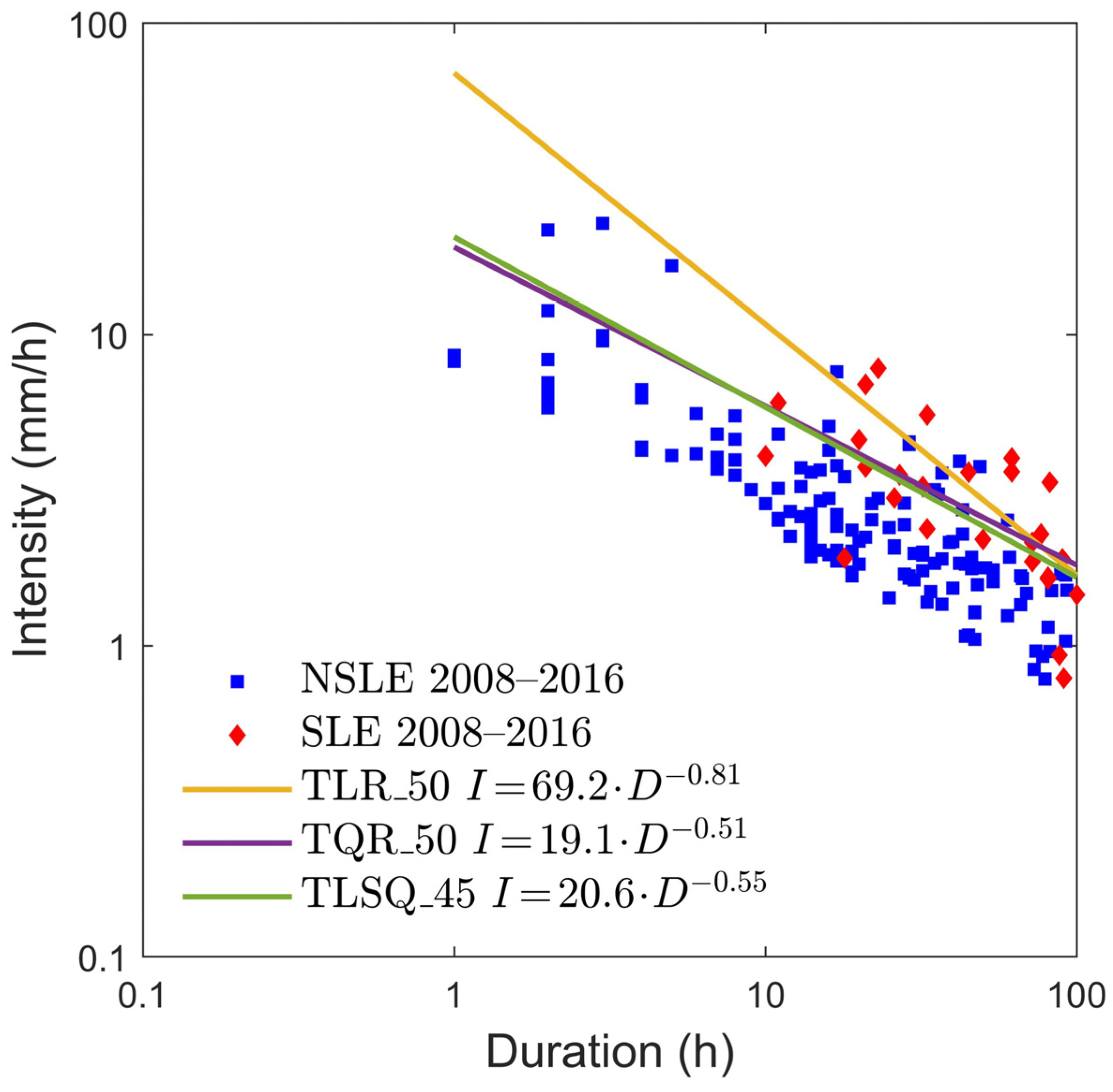
Figure 14.
Rainfall thresholds with maximum efficiency computed for the 2008–2016 period shown in
Table 14B obtained with the three different statistical methods. In this case there is a strong similarity between the QR and LSQ thresholds, reminiscent of the 1975–2002 period. Blue squares: events that did not triggered landslides (NSLE); red lozenges: events that triggered landslides (SLE).
Figure 15.
Rainfall thresholds obtained using the LR technique. Blue squares: events that did not trigger landslides (NSLE); red lozenges: events that triggered landslides (SLE).
Figure 15.
Rainfall thresholds obtained using the LR technique. Blue squares: events that did not trigger landslides (NSLE); red lozenges: events that triggered landslides (SLE).
Figure 16.
Rainfall thresholds obtained using the QR technique. Blue squares: events that did not trigger landslides (NSLE); red lozenges: events that triggered landslides (SLE).
Figure 16.
Rainfall thresholds obtained using the QR technique. Blue squares: events that did not trigger landslides (NSLE); red lozenges: events that triggered landslides (SLE).
Figure 17.
Rainfall thresholds obtained using the LSQ technique. Blue squares: events that did not triggered landslides (NSLE); red lozenges: events that triggered landslides (SLE).
Figure 17.
Rainfall thresholds obtained using the LSQ technique. Blue squares: events that did not triggered landslides (NSLE); red lozenges: events that triggered landslides (SLE).
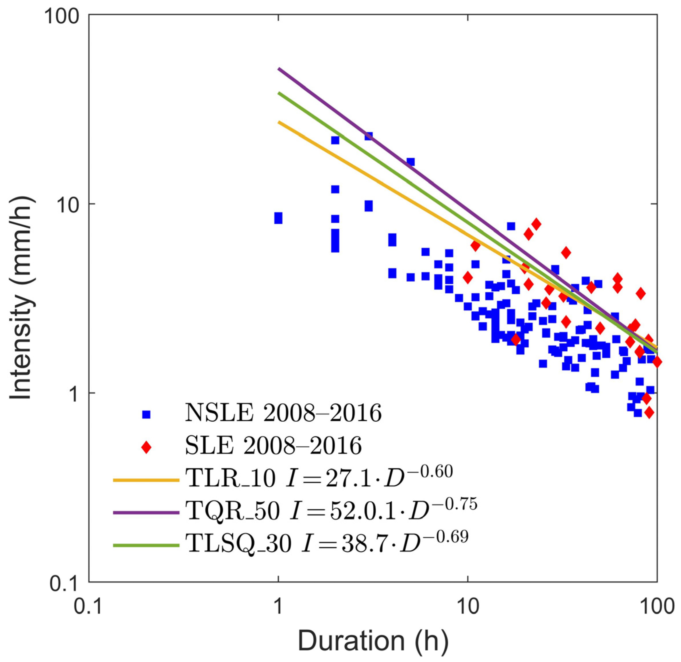
Figure 18.
The three rainfall thresholds with maximum efficiency computed using the combination of the rainfall data of the 2008–2016 period and the threshold parameters of the 1975–2002 period. Blue squares: events that did not triggered landslides (NSLE); red lozenges: events that triggered landslides (SLE).
Table 1.
Values of α and β for the 1975–2002 rainfall and landslide dataset obtained with the LR method for different landslide probability p (C.I.: confidence interval).
Table 1.
Values of α and β for the 1975–2002 rainfall and landslide dataset obtained with the LR method for different landslide probability p (C.I.: confidence interval).
| p | α | 95% C.I. for α | β | 95% C.I. for β |
|---|
| 0.01 | 16.0 | [8.63, 26.5] | −0.60 | [−0.70, −0.46] |
| 0.05 | 23.0 | [14.9, 33.2] | −0.60 | [−0.70, −0.46] |
| 0.10 | 27.1 | [18.9, 37.3] | −0.60 | [−0.70, −0.46] |
| 0.15 | 30.0 | [21.6, 40.1] | −0.60 | [−0.70, −0.46] |
| 0.20 | 32.4 | [24.2, 42.6] | −0.60 | [−0.70, −0.46] |
| 0.50 | 44.0 | [34.7, 55.1] | −0.60 | [−0.70, −0.46] |
Table 2.
Values of α and β for the 1975–2002 rainfall and landslide dataset obtained with the QR method for different exceeding probability pe (C.I.: confidence interval).
Table 2.
Values of α and β for the 1975–2002 rainfall and landslide dataset obtained with the QR method for different exceeding probability pe (C.I.: confidence interval).
| pe | α | 95% C.I. for α | β | 95% C.I. for β |
|---|
| 0.01 | 9.56 | [2.80, 32.6] | −0.33 | [−0.75, +0.085] |
| 0.05 | 28.4 | [8.36, 96.7] | −0.65 | [−1.0, −0.25] |
| 0.10 | 27.9 | [10.2, 76.7] | −0.60 | [−0.94, −0.27] |
| 0.15 | 27.6 | [14.4, 53.0] | −0.58 | [−0.80, −0.35] |
| 0.20 | 29.3 | [19.3, 44.2] | −0.60 | [−0.77, −0.43] |
| 0.50 | 52.0 | [32.8, 82.4] | −0.75 | [−0.94, −0.56] |
Table 3.
Values of α and β for the 1975–2002 rainfall and landslide dataset obtained with the LSQ method for different exceeding probability pe (C.I.: confidence interval).
Table 3.
Values of α and β for the 1975–2002 rainfall and landslide dataset obtained with the LSQ method for different exceeding probability pe (C.I.: confidence interval).
| pe | α | 95% C.I. for α | β | 95% C.I. for β |
|---|
| 0.01 | 17.4 | [11.8, 25.6] | −0.69 | [−0.87, −0.51] |
| 0.05 | 23.5 | [16.0, 34.7] | −0.69 | [−0.87, −0.51] |
| 0.10 | 27.7 | [18.8, 40.8] | −0.69 | [−0.87, −0.51] |
| 0.15 | 30.8 | [20.9, 45.4] | −0.69 | [−0.87, −0.51] |
| 0.20 | 33.6 | [22.8, 49.6] | −0.69 | [−0.87, −0.51] |
| 0.50 | 48.9 | [33.2, 72.0] | −0.69 | [−0.87, −0.51] |
Table 4.
Contingency table (TP, FN, FP, TN) and skill scores (POD, POFD, POFA, Ef, HK) of the thresholds obtained by LR method. Threshold showing the maximum efficiency value is highlighted in red.
Table 4.
Contingency table (TP, FN, FP, TN) and skill scores (POD, POFD, POFA, Ef, HK) of the thresholds obtained by LR method. Threshold showing the maximum efficiency value is highlighted in red.
| Threshold | p | TP | FN | FP | TN | POD | POFD | POFA | Ef | HK |
|---|
| TLR-5 | 0.05 | 27 | 1 | 81 | 58 | 0.964 | 0.583 | 0.750 | 0.509 | 0.382 |
| TLR-10 | 0.10 | 26 | 2 | 45 | 94 | 0.929 | 0.324 | 0.634 | 0.719 | 0.605 |
| TLR-30 | 0.30 | 16 | 12 | 19 | 120 | 0.571 | 0.137 | 0.543 | 0.814 | 0.435 |
| TLR-50 | 0.50 | 12 | 16 | 2 | 137 | 0.429 | 0.014 | 0.143 | 0.892 | 0.414 |
| TLR-55 | 0.55 | 12 | 16 | 1 | 138 | 0.429 | 0.007 | 0.077 | 0.898 | 0.421 |
| TLR-70 | 0.70 | 5 | 23 | 1 | 138 | 0.179 | 0.007 | 0.167 | 0.856 | 0.171 |
| TLR-90 | 0.90 | 2 | 26 | 0 | 139 | 0.071 | 0.000 | 0.000 | 0.844 | 0.071 |
Table 5.
Contingency table (TP, FN, FP, TN) and skill scores (POD, POFD, POFA, Ef, HK) of the thresholds obtained using QR method. Threshold showing the maximum efficiency value is highlighted in red (TQR_60 shows the same results but is calculated for a higher probability).
Table 5.
Contingency table (TP, FN, FP, TN) and skill scores (POD, POFD, POFA, Ef, HK) of the thresholds obtained using QR method. Threshold showing the maximum efficiency value is highlighted in red (TQR_60 shows the same results but is calculated for a higher probability).
| Threshold | pe | TP | FN | FP | TN | POD | POFD | POFA | Ef | HK |
|---|
| TQR_01 | 0.01 | 26 | 2 | 107 | 32 | 0.929 | 0.770 | 0.805 | 0.347 | 0.159 |
| TQR_05 | 0.05 | 27 | 1 | 57 | 82 | 0.964 | 0.410 | 0.679 | 0.653 | 0.554 |
| TQR_10 | 0.10 | 25 | 3 | 45 | 94 | 0.893 | 0.324 | 0.643 | 0.713 | 0.569 |
| TQR_15 | 0.15 | 25 | 3 | 36 | 103 | 0.893 | 0.259 | 0.590 | 0.766 | 0.634 |
| TQR_20 | 0.20 | 24 | 4 | 33 | 106 | 0.857 | 0.237 | 0.579 | 0.778 | 0.620 |
| TQR_50 | 0.50 | 13 | 14 | 13 | 126 | 0.481 | 0.094 | 0.500 | 0.837 | 0.388 |
| TQR_55 | 0.55 | 12 | 15 | 4 | 136 | 0.444 | 0.029 | 0.250 | 0.886 | 0.416 |
| TQR_60 | 0.60 | 12 | 15 | 4 | 136 | 0.444 | 0.029 | 0.250 | 0.886 | 0.416 |
| TQR_65 | 0.65 | 11 | 17 | 3 | 136 | 0.393 | 0.022 | 0.214 | 0.880 | 0.371 |
| TQR_90 | 0.90 | 2 | 26 | 0 | 139 | 0.071 | 0.000 | 0.000 | 0.844 | 0.071 |
Table 6.
Contingency table (TP, FN, FP, TN) and skill scores (POD, POFD, POFA, Ef, HK) of the thresholds obtained using LSQ method. Threshold showing the maximum efficiency value is highlighted in red.
Table 6.
Contingency table (TP, FN, FP, TN) and skill scores (POD, POFD, POFA, Ef, HK) of the thresholds obtained using LSQ method. Threshold showing the maximum efficiency value is highlighted in red.
| Threshold | pe | TP | FN | FP | TN | POD | POFD | POFA | Ef | HK |
|---|
| TLSQ_01 | 0.01 | 27 | 1 | 137 | 2 | 0.964 | 0.986 | 0.835 | 0.174 | −0.021 |
| TLSQ_05 | 0.05 | 27 | 1 | 115 | 24 | 0.964 | 0.827 | 0.810 | 0.305 | 0.137 |
| TLSQ_10 | 0.10 | 27 | 1 | 88 | 51 | 0.964 | 0.633 | 0.765 | 0.467 | 0.331 |
| TLSQ_15 | 0.15 | 26 | 2 | 67 | 72 | 0.929 | 0.482 | 0.720 | 0.587 | 0.447 |
| TLSQ_20 | 0.20 | 24 | 4 | 47 | 92 | 0.857 | 0.338 | 0.662 | 0.695 | 0.519 |
| TLSQ_50 | 0.50 | 14 | 14 | 9 | 130 | 0.500 | 0.065 | 0.391 | 0.862 | 0.435 |
| TLSQ_55 | 0.55 | 14 | 14 | 4 | 135 | 0.500 | 0.029 | 0.222 | 0.892 | 0.471 |
| TLSQ_60 | 0.60 | 11 | 17 | 3 | 136 | 0.393 | 0.022 | 0.214 | 0.880 | 0.371 |
| TLSQ_65 | 0.65 | 8 | 20 | 2 | 137 | 0.286 | 0.014 | 0.200 | 0.868 | 0.271 |
| TLSQ_90 | 0.90 | 2 | 26 | 0 | 139 | 0.071 | 0.000 | 0.000 | 0.844 | 0.071 |
Table 7.
Summary of the contingencies (TP, FN, FP, TN) and skill scores (POD, POFD, POFA, Ef, HK) of the SLE and NSLE forecasts obtained from the three best thresholds calculated on the 1975–2002 dataset using LR, LSQ, QR statistical techniques and the lower rainfall threshold plotted by [
27] (blue in
Figure 6). In this case, both the number of correct forecasts (28 out of 28 for SLE) and the number of false alarms (FP) are particularly high.
| Threshold | p, pe | TP | FN | FP | TN | POD | POFD | POFA | Ef | HK |
|---|
| Low T 2006 | - | 28 | 0 | 56 | 83 | 1.000 | 0.513 | 0.666 | 0.664 | 0.606 |
| TLR_55 | 0.55 | 12 | 16 | 1 | 138 | 0.429 | 0.007 | 0.077 | 0.898 | 0.421 |
| TQR_55 | 0.55 | 12 | 15 | 4 | 136 | 0.444 | 0.029 | 0.250 | 0.886 | 0.416 |
| TLSQ_55 | 0.55 | 14 | 14 | 4 | 135 | 0.500 | 0.029 | 0.222 | 0.892 | 0.471 |
Table 8.
Values of α and β for the 2008–2016 rainfall and landslide dataset obtained with the LR method for different landslide probability p (C.I.: confidence interval).
Table 8.
Values of α and β for the 2008–2016 rainfall and landslide dataset obtained with the LR method for different landslide probability p (C.I.: confidence interval).
| p | α | 95% C.I. for α | β | 95% C.I. for β |
|---|
| 0.01 | 17.6 | [9.73, 42.1] | −0.82 | [−1.1, −0.66] |
| 0.05 | 29.3 | [17.2, 63.9] | −0.82 | [−1.1, −0.66] |
| 0.10 | 36.9 | [21.2, 79.2] | −0.82 | [−1.1, −0.66] |
| 0.15 | 42.5 | [23.9, 99.7] | −0.82 | [−1.1, −0.66] |
| 0.20 | 47.4 | [26.5, 119] | −0.82 | [−1.1, −0.66] |
| 0.50 | 72.8 | [38.8, 193] | −0.82 | [−1.1, −0.66] |
Table 9.
Values of α and β for the 2008–2016 rainfall and landslide dataset obtained with the QR method for different exceeding probability pe (C.I.: confidence interval).
Table 9.
Values of α and β for the 2008–2016 rainfall and landslide dataset obtained with the QR method for different exceeding probability pe (C.I.: confidence interval).
| pe | α | 95% C.I. for α | β | 95% C.I. for β |
|---|
| 0.01 | 9.31 | [1.84, 47.0] | −0.55 | [−0.93, −0.17] |
| 0.05 | 7.29 | [1.72, 30.9] | −0.46 | [−0.81, −0.12] |
| 0.10 | 17.7 | [3.40, 91.7] | −0.64 | [−1.1, −0.23] |
| 0.15 | 17.7 | [3.67, 84.9] | −0.64 | [−1.1, −0.23] |
| 0.20 | 11.4 | [2.73, 47.1] | −0.45 | [−0.81, −0.079] |
| 0.50 | 19.1 | [8.37, 43.5] | −0.51 | [−0.71, −0.31] |
Table 10.
Values of α and β for the 2008–2016 rainfall and landslide dataset obtained with the LSQ method for different exceeding probability pe (C.I.: confidence interval).
Table 10.
Values of α and β for the 2008–2016 rainfall and landslide dataset obtained with the LSQ method for different exceeding probability pe (C.I.: confidence interval).
| pe | α | 95% C.I. for α | β | 95% C.I. for β |
|---|
| 0.01 | 8.17 | [3.86, 17.3] | −0.55 | [−0.73, −0.36] |
| 0.05 | 10.9 | [5.14, 23.0] | −0.55 | [−0.73, −0.36] |
| 0.10 | 12.7 | [5.98, 26.8] | −0.55 | [−0.73, −0.36] |
| 0.15 | 14.0 | [6.63, 29.7] | −0.55 | [−0.73, −0.36] |
| 0.20 | 15.2 | [7.20, 32.3] | −0.55 | [−0.73, −0.36] |
| 0.50 | 21.7 | [10.2, 45.9] | −0.55 | [−0.73, −0.36] |
Table 11.
Contingency table (TP, FN, FP, TN) and skill scores (POD, POFD, POFA Ef, HK) for the thresholds obtained by the LR method. The threshold showing the maximum efficiency (Ef = 0.885) is highlighted in red. NA: not available.
Table 11.
Contingency table (TP, FN, FP, TN) and skill scores (POD, POFD, POFA Ef, HK) for the thresholds obtained by the LR method. The threshold showing the maximum efficiency (Ef = 0.885) is highlighted in red. NA: not available.
| Threshold | p | TP | FN | FP | TN | POD | POFD | POFA | Ef | HK |
|---|
| TLR_5 | 0.05 | 29 | 2 | 81 | 71 | 0.935 | 0.533 | 0.736 | 0.546 | 0.403 |
| TLR_10 | 0.10 | 27 | 4 | 57 | 95 | 0.871 | 0.375 | 0.679 | 0.667 | 0.496 |
| TLR_30 | 0.30 | 18 | 13 | 19 | 133 | 0.581 | 0.125 | 0.514 | 0.825 | 0.456 |
| TLR_50 | 0.50 | 13 | 18 | 3 | 149 | 0.419 | 0.020 | 0.188 | 0.885 | 0.400 |
| TLR_70 | 0.70 | 7 | 24 | 0 | 152 | 0.226 | 0.000 | 0.000 | 0.869 | 0.226 |
| TLR_90 | 0.90 | 0 | 31 | 0 | 152 | 0.000 | 0.000 | NA | 0.831 | 0.000 |
Table 12.
Contingency table (TP, FN, FP, TN) and skill scores (POD, POFD, POFA Ef, HK) for the thresholds obtained using the QR method. Although the threshold relating to the ninetieth percentile of exceedance probability shows the highest efficiency (Ef = 0.852), the threshold highlighted in red was considered better for the higher POD and HK parameters.
| Threshold | pe | TP | FN | FP | TN | POD | POFD | POFA | Ef | HK |
|---|
| TQR_01 | 0.01 | 31 | 0 | 130 | 22 | 1.000 | 0.855 | 0.807 | 0.290 | 0.145 |
| TQR_05 | 0.05 | 28 | 3 | 128 | 24 | 0.903 | 0.842 | 0.821 | 0.284 | 0.061 |
| TQR_10 | 0.10 | 28 | 3 | 69 | 83 | 0.903 | 0.454 | 0.711 | 0.607 | 0.449 |
| TQR_15 | 0.15 | 28 | 3 | 69 | 83 | 0.903 | 0.454 | 0.711 | 0.607 | 0.449 |
| TQR_20 | 0.20 | 25 | 5 | 38 | 114 | 0.833 | 0.250 | 0.603 | 0.764 | 0.583 |
| TQR_50 | 0.50 | 15 | 16 | 13 | 139 | 0.484 | 0.086 | 0.464 | 0.842 | 0.398 |
| TQR_55 | 0.55 | 13 | 18 | 12 | 140 | 0.419 | 0.079 | 0.480 | 0.836 | 0.340 |
| TQR_60 | 0.60 | 13 | 18 | 11 | 141 | 0.419 | 0.072 | 0.458 | 0.842 | 0.347 |
| TQR_65 | 0.65 | 10 | 21 | 10 | 142 | 0.323 | 0.066 | 0.500 | 0.831 | 0.257 |
| TQR_90 | 0.90 | 4 | 27 | 0 | 152 | 0.129 | 0.000 | 0.000 | 0.852 | 0.129 |
Table 13.
Contingency table (TP, FN, FP, TN) and skill scores (POD, POFD, POFA, Ef, HK) of the thresholds obtained using the LSQ method. Maximum efficiency value is reached with the threshold highlighted in red relating to an exceedance probability of 0.45 (Ef = 0.852).
Table 13.
Contingency table (TP, FN, FP, TN) and skill scores (POD, POFD, POFA, Ef, HK) of the thresholds obtained using the LSQ method. Maximum efficiency value is reached with the threshold highlighted in red relating to an exceedance probability of 0.45 (Ef = 0.852).
| Threshold | pe | TP | FN | FP | TN | POD | POFD | POFA | Ef | HK |
|---|
| TLSQ_01 | 0.01 | 31 | 0 | 152 | 0 | 1.000 | 1.000 | 0.831 | 0.169 | 0.000 |
| TLSQ_05 | 0.05 | 28 | 3 | 97 | 55 | 0.903 | 0.638 | 0.776 | 0.454 | 0.265 |
| TLSQ_10 | 0.10 | 27 | 4 | 75 | 77 | 0.871 | 0.493 | 0.735 | 0.568 | 0.378 |
| TLSQ_15 | 0.15 | 27 | 4 | 59 | 93 | 0.871 | 0.388 | 0.686 | 0.656 | 0.483 |
| TLSQ_20 | 0.20 | 26 | 5 | 45 | 107 | 0.839 | 0.296 | 0.634 | 0.727 | 0.543 |
| TLSQ_45 | 0.45 | 18 | 13 | 14 | 138 | 0.581 | 0.092 | 0.438 | 0.852 | 0.489 |
| TLSQ_50 | 0.50 | 16 | 15 | 13 | 139 | 0.516 | 0.086 | 0.448 | 0.847 | 0.431 |
| TLSQ_55 | 0.55 | 13 | 18 | 11 | 141 | 0.419 | 0.072 | 0.458 | 0.842 | 0.347 |
| TLSQ_60 | 0.60 | 10 | 21 | 9 | 143 | 0.323 | 0.059 | 0.474 | 0.836 | 0.263 |
| TLSQ_65 | 0.65 | 9 | 22 | 9 | 143 | 0.290 | 0.059 | 0.500 | 0.831 | 0.231 |
| TLSQ_90 | 0.90 | 4 | 27 | 2 | 150 | 0.129 | 0.013 | 0.333 | 0.842 | 0.116 |
Table 14.
Summary of contingencies and efficiency values (Ef) of the forecasts of SLEs and NSLEs using the three best thresholds computed on the 2008–2016 dataset before (
A) and after (
B) the reduction of the dataset shown in
Figure 8 and
Figure 9.
Table 14.
Summary of contingencies and efficiency values (Ef) of the forecasts of SLEs and NSLEs using the three best thresholds computed on the 2008–2016 dataset before (
A) and after (
B) the reduction of the dataset shown in
Figure 8 and
Figure 9.
| | Threshold | p, pe | TP | FN | FP | TN | Ef |
|---|
| A | LR_50 | 0.50 | 13 | 18 | 3 | 533 | 0.963 |
| LSQ_45 | 0.45 | 18 | 13 | 4 | 522 | 0.952 |
| QR_50 | 0.50 | 15 | 16 | 13 | 523 | 0.949 |
| B | LR_50 | 0.50 | 13 | 18 | 3 | 149 | 0.885 |
| LSQ_45 | 0.45 | 18 | 13 | 4 | 138 | 0.852 |
| QR_50 | 0.50 | 15 | 16 | 13 | 139 | 0.842 |
Table 15.
Contingency table (TP, FN, FP, TN) and skill scores (POD, POFD, POFA Ef, HK) for the dataset of the 2008–2016 period and the rainfall thresholds calculated regarding the 1975–2002 dataset obtained using the LR method. Maximum efficiency value is reached with the curve highlighted in red relating to a landslide probability of 0.1 (Ef = 0.858). NA: not available.
| Threshold | p | TP | FN | FP | TN | POD | POFD | POFA | Ef | HK |
|---|
| TLR_5 | 0.05 | 20 | 11 | 17 | 135 | 0.645 | 0.112 | 0.459 | 0.847 | 0.533 |
| TLR_10 | 0.10 | 15 | 16 | 10 | 142 | 0.484 | 0.066 | 0.400 | 0.858 | 0.418 |
| TLR_30 | 0.30 | 7 | 24 | 4 | 148 | 0.226 | 0.026 | 0.364 | 0.847 | 0.199 |
| TLR_50 | 0.50 | 5 | 26 | 0 | 152 | 0.161 | 0.000 | 0.000 | 0.858 | 0.161 |
| TLR_70 | 0.70 | 0 | 31 | 0 | 152 | 0.000 | 0.000 | NA | 0.831 | 0.000 |
| TLR_90 | 0.90 | 0 | 31 | 0 | 152 | 0.000 | 0.000 | NA | 0.831 | 0.000 |
Table 16.
Contingency table (TP, FN, FP, TN) and skill scores (POD, POFD, POFA Ef, HK) for the 2008–2016 dataset and the thresholds calculated regarding the data relating to the 1975–2002 period obtained using the QR method. Maximum efficiency value is reached with the curve highlighted in red relating to an exceedance probability of 0.5 (Ef = 0.863), which is considered better for the higher POD and HK parameters.
| Threshold | pe | TP | FN | FP | TN | POD | POFD | POFA | Ef | HK |
|---|
| TLR_01 | 0.01 | 14 | 17 | 26 | 126 | 0.452 | 0.171 | 0.650 | 0.765 | 0.281 |
| TLR_05 | 0.05 | 19 | 12 | 18 | 134 | 0.613 | 0.178 | 0.486 | 0.836 | 0.494 |
| TLR_10 | 0.10 | 14 | 17 | 10 | 142 | 0.452 | 0.066 | 0.417 | 0.852 | 0.386 |
| TLR_15 | 0.15 | 11 | 20 | 9 | 143 | 0.355 | 0.059 | 0.450 | 0.842 | 0.296 |
| TLR_20 | 0.20 | 12 | 19 | 9 | 143 | 0.387 | 0.059 | 0.429 | 0.847 | 0.328 |
| TLR_50 | 0.50 | 14 | 17 | 8 | 144 | 0.452 | 0.053 | 0.364 | 0.863 | 0.399 |
| TLR_55 | 0.55 | 7 | 24 | 1 | 151 | 0.226 | 0.007 | 0.125 | 0.863 | 0.219 |
| TLR_60 | 0.60 | 7 | 24 | 1 | 151 | 0.226 | 0.007 | 0.125 | 0.863 | 0.219 |
| TLR_65 | 0.65 | 7 | 24 | 0 | 152 | 0.226 | 0.000 | 0.000 | 0.869 | 0.226 |
| TLR_90 | 0.90 | 5 | 26 | 0 | 152 | 0.161 | 0.000 | 0.000 | 0.858 | 0.161 |
Table 17.
Contingency table (TP, FN, FP, TN) and skill scores (POD, POFD, POFA, Ef, HK) for the 2008–2016 dataset period and the thresholds calculated on the data relating to the 1975–2002 period obtained using the LSQ method. Maximum efficiency value is reached with the curve highlighted in red relating to an exceedance probability of 0.30 (Ef = 0.858). NA: not available.
| Threshold | pe | TP | FN | FP | TN | POD | POFD | POFA | Ef | HK |
|---|
| TLR_01 | 0.01 | 30 | 1 | 92 | 60 | 0.968 | 0.605 | 0.754 | 0.492 | 0.362 |
| TLR_05 | 0.05 | 26 | 5 | 51 | 101 | 0.839 | 0.336 | 0.662 | 0.694 | 0.503 |
| TLR_10 | 0.10 | 25 | 6 | 31 | 121 | 0.806 | 0.204 | 0.554 | 0.798 | 0.603 |
| TLR_15 | 0.15 | 23 | 8 | 24 | 128 | 0.742 | 0.158 | 0.511 | 0.825 | 0.584 |
| TLR_20 | 0.20 | 20 | 11 | 22 | 130 | 0.645 | 0.145 | 0.524 | 0.820 | 0.500 |
| TLR_30 | 0.30 | 14 | 17 | 9 | 143 | 0.452 | 0.059 | 0.391 | 0.858 | 0.392 |
| TLR_50 | 0.50 | 9 | 22 | 4 | 148 | 0.290 | 0.026 | 0.308 | 0.858 | 0.264 |
| TLR_55 | 0.55 | 8 | 23 | 2 | 150 | 0.258 | 0.013 | 0.200 | 0.863 | 0.245 |
| TLR_60 | 0.60 | 7 | 24 | 0 | 152 | 0.226 | 0.000 | 0.000 | 0.869 | 0.226 |
| TLR_65 | 0.65 | 6 | 25 | 0 | 152 | 0.194 | 0.000 | 0.000 | 0.863 | 0.194 |
| TLR_90 | 0.90 | 0 | 31 | 0 | 152 | 0.000 | 0.000 | NA | 0.831 | 0.000 |
Table 18.
Summary of the contingencies and the skill scores of the forecasts of the SLEs and NSLEs using the three best thresholds computed with the threshold parameters of the 1975–2002 dataset combined with the 2008–2016 dataset.
Table 18.
Summary of the contingencies and the skill scores of the forecasts of the SLEs and NSLEs using the three best thresholds computed with the threshold parameters of the 1975–2002 dataset combined with the 2008–2016 dataset.
| Threshold | p, pe | TP | FN | FP | TN | POD | POFD | POFA | Ef | HK |
|---|
| TLR_10 | 0.10 | 15 | 16 | 10 | 142 | 0.484 | 0.066 | 0.400 | 0.858 | 0.418 |
| TQR_50 | 0.50 | 14 | 17 | 8 | 144 | 0.452 | 0.053 | 0.364 | 0.863 | 0.399 |
| TLSQ_30 | 0.30 | 14 | 17 | 9 | 143 | 0.452 | 0.059 | 0.391 | 0.858 | 0.392 |


