Correlation between Turbidity and Inherent Optical Properties as an Initial Recognition for Backscattering Coefficient Estimation

Abstract

Seawater turbidity is a common water quality indicator measured in situ and estimated from space on a regular basis. However, it is rarely correlated with the inherent optical properties of seawater, which convey information about seawater composition. In this study, we show a simple application of the turbidimeter’s weighting function in the estimation of the backscattering coefficient of a model inorganic suspension in seawater. First, we introduce a method to measure the instrument’s weighting function which describes the sensor’s angular response in terms of scattering angles. The determination of the sensor-specific weighting function led us to characterize its angular sensitivity to the presence of suspended particles. The highest sensitivity for the Seapoint turbidimeter is in the range of 114°–128° (containing 25% of the total signal). Next, we describe the correlations between turbidity and the scattering and backscattering coefficients on the example of the model of inorganic particle suspension using the calculations based on Mie theory. The correlations are analyzed for narrow size fractions of the particle size distribution of silica in the range of 0.59–190 µm. We established that there is a good linear correlation (characterized by the coefficient of determination r² = 0.979) between the part of the scattering coefficient measured by the turbidimeter and the backscattering coefficient of all size fractions of the model inorganic suspension.

1. Introduction

According to the Water Framework Directive [1], the quality elements for the classification of ecological status include thermal, oxygenation, and nutrient conditions, as well as salinity, acidification status, and transparency. The oldest and still popular method of measuring water transparency is the determination of the Secchi depth (SD) by lowering the Secchi disk (white or black and white disk with a diameter of 20–30 cm) into the water until it is no longer visible to the observer [2,3]. The SD describes the spatial variability of water properties and is closely related to the absorption and scattering of underwater light [4]. It is widely accepted as a good indicator of eutrophication [5].

Nowadays, both transparency and turbidity are well-known indicators of water quality [6]. Widely available multiparameter underwater probes are equipped with modern sensors for measuring turbidity, which express the scattered light resulting from the interaction of incident light with particulate material in a liquid sample [7,8]. The scattering process changes the direction of light rays on randomly distributed optical inhomogeneities of the medium [9]. In the natural marine environment, such inhomogeneities are suspended in dissolved substances: clay, silt, pine pollen, finely divided organic matter, plankton, other microscopic organisms, floating debris, oil droplets, organic acids, pigments, and air bubbles [7,10,11,12,13,14,15]. The increase in the amount of admixed components reduces water quality and transparency and, consequently, causes higher turbidity levels. The size of suspension particles or bubbles has a significant influence on optical measurements, including turbidity measurements [7,16,17,18].

A device that measures turbidity is called a turbidimeter. Currently, there is a large selection of turbidimeters on the market, which are generally categorized as absorptiometers and nephelometers [13,19]. The measurements can be performed in the laboratory on collected water samples, taken from the ship in the entire section of the water column, or can be constantly recorded by a sensor installed on a hydrographic platform or buoy. Turbidimeters have various designs and modes of operation—based on attenuation or scattering detection, different light sources, beam configurations, angular range, and the spectral sensitivity of detectors [17,19,20,21].

Raw data from differently designed instruments should not be considered directly interchangeable as the turbidity reporting units correspond with turbidity sensor design. This means that the turbidity, measured with instruments of different optical configurations, may differ for the same environmental sample [13,17,22,23]. A detailed compilation of turbidity reporting units (

Table 1. Reporting units corresponding to turbidity instrument designs (Table 6.7–4. in [17]).

Detector Geometry	Light Wavelength
	White or Broadband (with a Peak Spectral Output of 400–680 nm)	Monochrome (Spectral Output Typically Near-Infrared, 780–900 nm)
Single Illumination Beam Light Source
At 90° to the incident beam	Nephelometric Turbidity Unit (NTU) 1 (P63675)	Formazin Nephelometric Unit (FNU) 2 (P63680)
At 90° and other angles. An instrument algorithm uses a combination of detector readings, which may differ for values of varying magnitude	Nephelometric Turbidity Ratio Unit (NTRU) (P63676)	Formazin Nephelometric Ratio Unit (FNRU) (P63681)
At 30° ± 15° to the incident beam (backscatter)	Backscatter Unit (BU) (P63677)	Formazin Backscatter Unit (FBU) (P63682)
At 180° to the incident beam (attenuation)	Attenuation Unit (AU) (P63678)	Formazin Attenuation Unit (FAU) (P63683)
Multiple illumination beam light source
At 90° and possibly other angles to each beam. An instrument algorithm uses a combination of detector readings, which may differ for values of varying magnitude	Nephelometric Turbidity Multibeam Unit (NTMU) (P63679)	Formazin Nephelometric Multibeam Unit (FNMU) (P63684)

¹ EPA Method 180.1 defines the optical geometry for NTU measurements. The detector angle must be 90° ± 30 to the incident light beam. The light source must be a tungsten lamp with a color temperature of 2200–3000 K [24]. ² ISO 7027 defines the optical geometry for FNU measurements. The detector angle must be 90° ± 2.5 to the incident light beam. The light source must be a light-emitting diode (LED) with a wavelength of 860 ± 60 nm [25].

) was provided by Anderson [17].

A comprehensive overview of turbidimeters, their operating principles, and stated accuracies was presented by Rymszewicz [19], who tested twelve commercially available instruments to assess their traceability in comparison with previously prepared suspensions with known suspended solids concentrations. This experiment showed a large discrepancy in the responses of optical turbidimeters, regardless of the principle of their operation. It is considered that the 90° detection angle is the most sensitive angle to measure scattered light, characterized by the quasi-linear correlation between turbidity and light intensity for small turbidity values [16,22].Thus, turbidity is most commonly expressed in a NTU (Nephelometric Turbidity Unit) or FNU (Formazin Nephelometric Unit). In the existing literature related to the study of the natural environment, the results of turbidity measurements are most often expressed in these units [23,24]. However, in some papers, the authors measure and analyze turbidity in Formazin Turbidity Units (FTU) [12,25,26,27]. The FTU became a defined unit after the acceptance of Formazin as the primary reference standard for turbidity measurement, however, the FTU does not specify how a device measures turbidity in a water sample. Still, there is a lack of specificity in the influence of the ambient conditions and sensor configuration on the measurements in different instruments [28,29].

Turbidity measurements in natural ocean waters typically provide results in the range of below 1 NTU for oligotrophic waters to several NTU for eutrophic waters depending on chlorophyll concentration. These values for coastal waters can be as high as 10 NTU, while in estuaries they may exceed 100 NTU [29,30] or even 10,000 NTU in extremely turbid waters [31]. Typical turbidity values in natural open sea waters allow us to assume with a good approximation that in the range of optical path, which in most turbidimeters is 1–10 cm long, there will be no phenomenon of particle obscuration or multiple scattering. This is why we can assume that turbidity is a measurement of a fragment of the volume scattering function (VSF), around the scattering angle of 90°. Therefore, there is a question of whether the measurement made with a turbidimeter can be described by the inherent optical properties (IOPs) of ocean water.

To address this question, this study focused on the following research objectives:

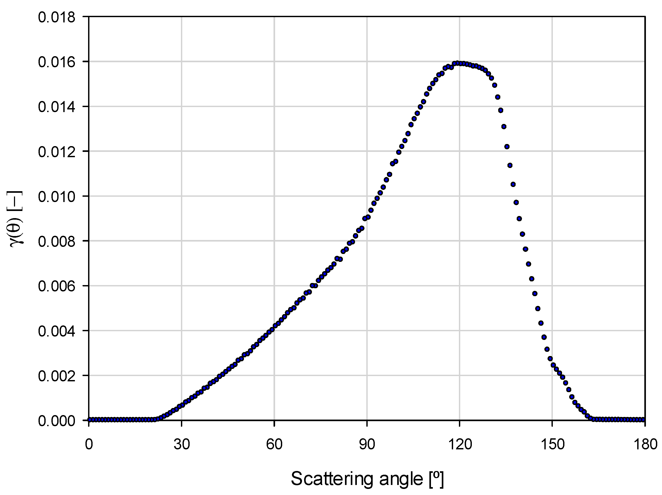
• Determining the angular weighting function that would define what part of the volume scattering function is recorded by the turbidity meter. This function will be defined as γ(θ) in the next chapter;
• Determining angular scattering properties, as well as the magnitude of the signal, measured by the turbidity meter for different fractions of the model suspension;
• Finding the correlation of the turbidimeter signal with elements of the scattering properties of the suspension.

2. Materials and Methods

2.1. Mathematical Description of Turbidity under Single Scattering Regime

In environmental optics, the light scattering coefficient of suspended particulate matter (b_p) measured in m⁻¹ is applied to describe the optical properties of the analyzed medium [9,32]. Due to the assumed homogeneity of scattering around the optical axis, the b_p is defined as the integral of the volume scattering function (VSF) over the full solid angle:

$$b_p=2\pi {\int }_0^{\pi }{\beta }_p\left(\theta \right)·sin\theta d\theta ,$$

(1)

where β_p(θ) is the particle VSF of scatterers and θ is the scattering angle. The backscattering coefficient (b_bp) is defined as the integral of the VSF over the scattering angles of 90° to 180°:

$$b_{bp}=2\pi {\int }_{\pi /2}^{\pi }{\beta }_p\left(\theta \right)·sin\theta d\theta .$$

(2)

The quotient of the particle backscattering coefficient and the scattering coefficient called the backscattering ratio (B_p), describes the probability that, as a result of scattering, a photon will hit the backward hemisphere, and it is defined as:

$$B_p=\frac{b_{bp}}{b_p}$$

(3)

A turbidimeter measures the intensity of light scattered into some angles. Depending on the relative position of the sample illumination window and the detector window, as well as the shape of the measurement chamber, the angles at which the scattered light reaches the detector can be characterized using various weighting functions $\gamma \left(\theta \right)$. Using the inherent optical properties, the signal registered by the turbidimeter (b_turb), may be described by the following part of the scattering coefficient b_p:

$$b_{turb}=2\pi {\int }_0^{\pi }{\beta }_p\left(\theta \right)\cdot \gamma \left(\theta \right)\cdot sin\theta d\theta$$

(4)

where γ(θ) is a dimensionless weighting function of the turbidimeter, which depends on the scattering angle θ. In fact, this dimensionless function describes the angular probability distribution of the turbidity measurement made under single scattering conditions. It is unique for every device and provides information on the contribution of recorded signals from different angles. In our experiment, γ(θ) was determined during laboratory tests (Section 2.2). The determination of the turbidimeter’s weighting function allows us to link turbidity measurement to the inherent optical properties of the water sample.

Under single scattering conditions, when the detector receives light from scattering on the first suspended particle encountered in a water sample, the turbidity signal (T) will be proportional to the part of the scattering coefficient defined above as b_turb:

$$b_{turb}=const·T$$

(5)

For turbidity T measured in FTU, the proportionality factor would be expressed in FTU⁻¹·m⁻¹.

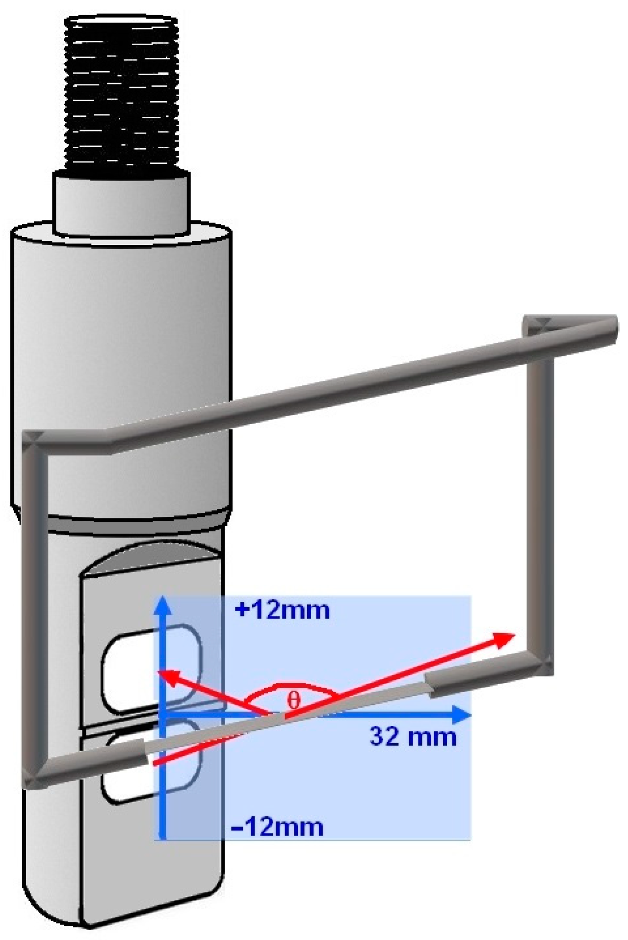
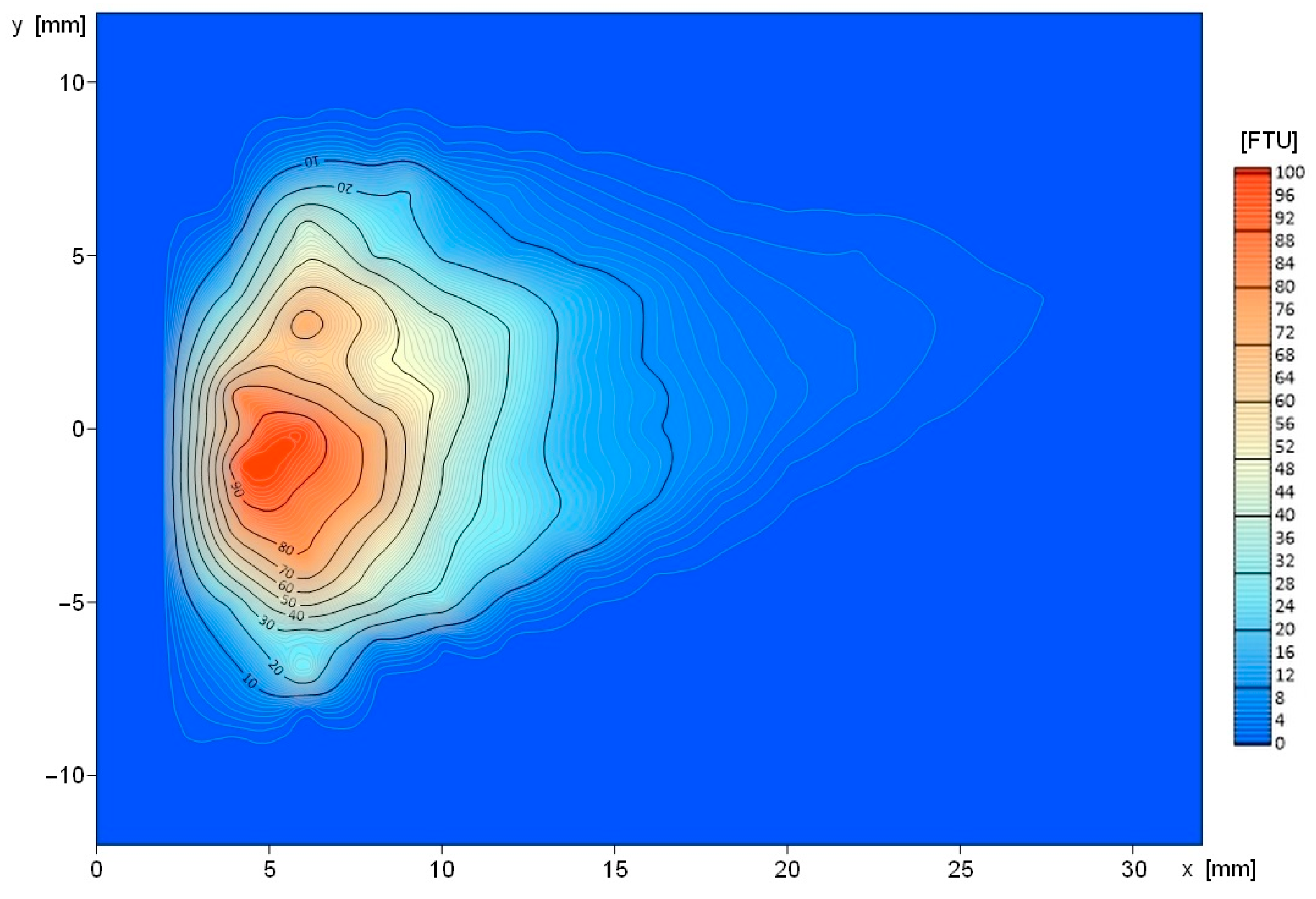
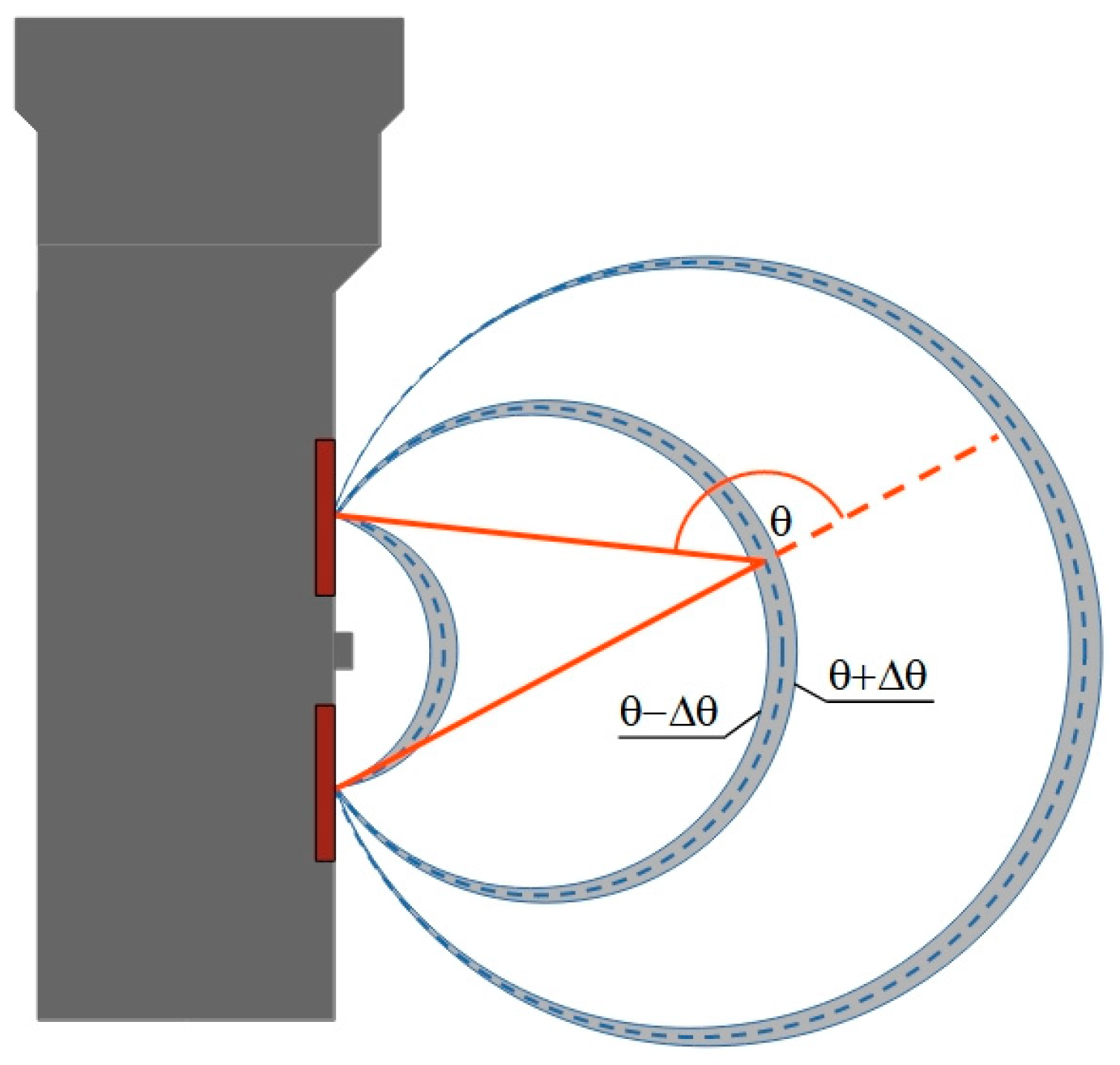
2.2. Measurements of the Angular Weighting Function

For the experiment, the SAIV SD204 CTD/STD probe (SAIV A/S, Bergen, Norway) was used, which was equipped with a turbidity meter manufactured by Seapoint Sensors Inc. (Exeter, NH, USA). It is a small-size turbidity sensor suitable for in-water measurements up to 6000 m depth characterized by a low-temperature coefficient of <0.05%/°C and a relatively low sensing distance of 5 cm from optical windows. The sensor can be operated in four selectable ranges: 12.5, 62.5, 250, and 750 FTU—characterized by supplier-declared signal linearity of <2% deviation in the range of 0–1250 FTU. The instrument is equipped with an LED light source that emits a light wavelength of 880 nm (near-infrared range). Detectors are silicon photodiodes with visible-light-blocking filters. Thus, the detector can register light scattered by sample particles at angles of 15° to 150°.

The determination of the gamma function was based on measurements taken on a specially prepared test stand (Figure 1). In front of the probe, a 0.5 mm thick and 10 cm long steel rod was placed, which was mounted on a frame that could be shifted up and down, as well as moved towards and away from the optical windows. The probe recorded turbidity values generated by the steel rod (T_rod). The sliders were equipped with fine threads enabling the reading of changes in the position of the rod with an accuracy of 0.02 mm. The turbidity sensor and the sliding bar were immersed in MilliQ water.

Measurements were taken in an area of 24 × 32 mm covering the turbidimeter field of view. The majority of measurements were made within a range of 62.5 FTU, however, after bringing the rod to the windows at a distance of less than 8 mm, the recorded signal exceeded the originally selected range. Measurements in the square area of 8 × 8 mm closest to the turbidimeter windows were made within a range of 250 FTU. Turbidity was recorded every 1 mm in a vertical direction and every 2 mm in a horizontal direction.

2.3. Model of Inorganic Particle Suspension

To demonstrate the application of the angular weighting function of the turbidimeter, a model particle suspension was developed and mathematical calculations of the inherent optical properties were performed based on the Mie solution [33]. This is the solution to Maxwell’s equations (also known as the Lorenz-Mie solution) and describes the scattering of an electromagnetic wave on homogeneous spheres. The solution was suggested by Gustav Mie a long time ago, in 1908 [33], but it was not until the use of computer algorithms [34] that the calculations could be repeatedly duplicated for a wide range of scattering particle sizes. Thus, Mie scattering could be used as a scattering approximation for aerosols and aqueous suspensions.

According to the assumptions of the Mie solution, a homogeneous suspension of inorganic spherical particles was developed, which was characterized by a particle size distribution (PSD) similar to the natural distributions in the marine environment. The PSD of our model suspension is described by the power–law function according to [35]. This function was approximated using the single-segment power law:

$$PSD\left(d\right)=1.17·{10}^5·d^{-4.25},$$

(6)

where d is the particle diameter and PSD is the number of particles in 1 cubic centimeter per 1 μm range of particle diameters.

Next, we divided this particle size distribution into 22 narrow-size fractions starting from 0.59 μm with a multiplier of 1.3. The first fraction had a diameter range of 0.59 to 0.77 μm, and the last one of 146 to 190 μm. Each fraction was, therefore, assigned a different concentration of particles (see

Table 2. The concentration of particles, scattering, and backscattering coefficients for each of the 22 fractions of PSD.

Fraction Number	Diameter Range [μm]	Concentration [m−3]	Scattering Coefficient bp [m−1]	Backscattering Coefficient bbp [m−1]
1	0.59–0.77	1.13 × 1011	7.16 × 10−3	1.69 × 10−4
2	0.77–1	4.85 × 1010	9.18 × 10−3	1.16 × 10−4
3	1–1.30	2.07 × 1010	1.13 × 10−2	9.42 × 10−5
4	1.30–1.69	8.80 × 109	1.37 × 10−2	7.28 × 10−5
5	1.69–2.20	3.75 × 109	1.59 × 10−2	6.11 × 10−5
6	2.20–2.86	1.60 × 109	1.74 × 10−2	5.10 × 10−5
7	2.86–3.71	6.82 × 108	1.74 × 10−2	4.51 × 10−5
8	3.71–4.83	2.91 × 108	1.45 × 10−2	4.06 × 10−5
9	4.83–6.28	1.24 × 108	8.78 × 10−3	3.67 × 10−5
10	6.28–8.16	5.28 × 107	3.85 × 10−3	3.38 × 10−5
11	8.16–10.6	2.25 × 107	2.73 × 10−3	3.09 × 10−5
12	10.6–13.8	9.60 × 106	2.43 × 10−3	2.90 × 10−5
13	13.8–17.9	4.09 × 106	1.41 × 10−3	2.22 × 10−5
14	17.9–23.3	1.74 × 106	1.03 × 10−3	1.32 × 10−5
15	23.3–30.3	7.43 × 105	7.14 × 10−4	5.67 × 10−6
16	30.3–39.4	3.17 × 105	4.94 × 10−4	2.85 × 10−6
17	39.4–51.2	1.35 × 105	3.31 × 10−4	1.66 × 10−6
18	51.2–66.5	5.76 × 104	2.33 × 10−4	7.77 × 10−7
19	66.5–86.5	2.45 × 104	1.63 × 10−4	3.94 × 10−7
20	86.5–112	1.05 × 104	1.20 × 10−4	2.06 × 10−7
21	112–146	4.46 × 103	9.27 × 10−5	1.23 × 10−7
22	146–190	1.90 × 103	7.24 × 10−5	8.12 × 10−8

). Then, for every size fraction, the b_p and the VSF were computed. Despite the assumption of ideal sphericity of particles, the application of the Mie solution provides precise results, particularly for particles with surface irregularities smaller than the wavelength of 880 nm. The optical properties of the model inorganic suspension are determined by its complex refractive index [35]. Clay minerals are the most typical inorganic substances found in natural water bodies. They are composed essentially of silica with the addition of aluminum, magnesium, or iron in varying degrees, and sometimes potassium, sodium, and calcium [36]. This is why we chose silica (SiO₂) as the representative compound, which can be found in large amounts in the natural inorganic suspension.

The Seapoint turbidimeter is powered by infrared light with a wavelength of 880 nm and at this wavelength, the refractive index of silica is n = 1.45998, and the imaginary part is k = 0.0011858i [37]. Both the particle size distribution and the complex refractive index were the input data for the Mie calculations.

3. Results

3.1. The Turbidimeter’s Angular Weighting Function

The turbidimeter’s weighting function was measured to characterize the strength of the output signal received from different angles. While moving the steel rod in the vertical and horizontal planes, turbidity values T_rod in FTU were recorded. The resulting data set was interpolated using the kriging method in the Surfer by Golden software program to obtain the vertical cross-section of the turbidity distribution (Figure 2). The measured values varied from 0.39 FTU on the periphery of the area analyzed to as much as 97.38 FTU recorded at a distance of 6 mm from the probe at the central height between the emitter and the detector windows. The minimal value of 0.39 FTU was taken as the measurement background and subtracted from all results so that the measured values represented only the result of infrared light scattering from the rod.

Converting the spatial turbidity distribution into an angular probability function required a linear interpolation between the points. After linear interpolation, made in MATLAB, results were obtained for a grid with a pixel size of 0.02 mm. For each of these pixels, the angle between the centers of the two turbidimeter windows was determined. Pixels were assigned the same scattering angle lie on arcs, passing through the centers of the illuminating and recording windows (see Figure 3). Interpolated turbidity values T_rod were integrated for each angle range of θ − Δθ to θ + Δθ and normalized to unity according to the formula:

$$\gamma \left(\theta \right)=\frac{{\int }_{\theta -\mathsf{\Delta }\theta }^{\theta +\mathsf{\Delta }\theta }{T}_{rod}d\theta }{{\int }_0^{\pi }{T}_{rod}d\theta },$$

(7)

where interval Δθ was set as 0.5°.

The obtained function is the turbidimeter’s weighting function, plotted in Figure 4. The weighting function γ(θ) indicates the range of scattering angles measured by the sensor and depends only on the instrument and not on the suspended particles in the sample. It characterizes the angles which have the greatest contributions to the measured value. For the Seapoint turbidimeter, it takes the values below 10⁻⁴ for angles lower than 18° and above 156°. The highest value, which is 0.0159, is obtained for an angle of 120°. The resulting peak is also characterized by an extensive full width at half maximum (FWHM) of 55°.

Moreover, the obtained weighting function shows that the Seapoint turbidimeter has the highest sensitivity for scattering angles in a range of 114°–128°, which contains 25% of the signal. Half of the sensitivity falls in an angular range of 102°–134°. Three-quarters (75%) are located in a range of 84°–140°, and 90% in a wide range of scattering angles of 62° to 146°. Therefore, we can see a large asymmetry in the weighting function, which slopes more steeply for angles higher than 128°. This is 2.75 times less than the Seapoint turbidity meter’s weighting function.

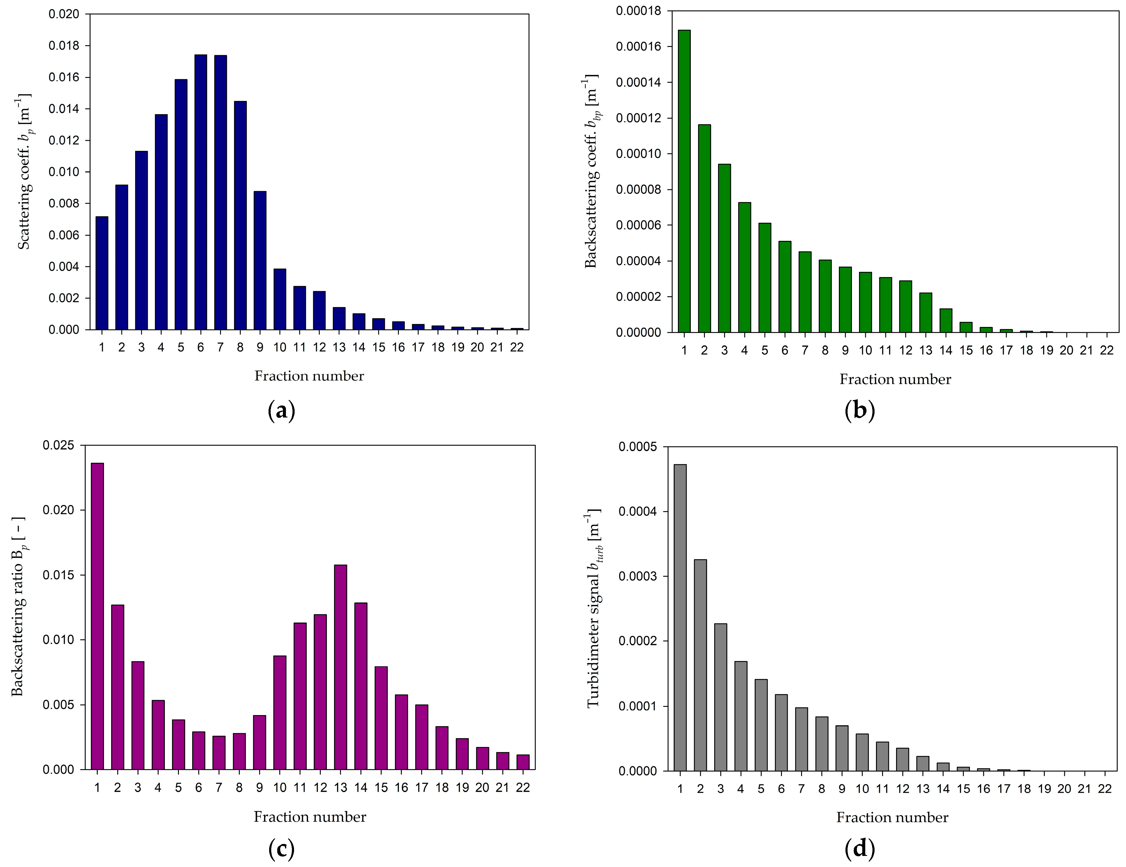
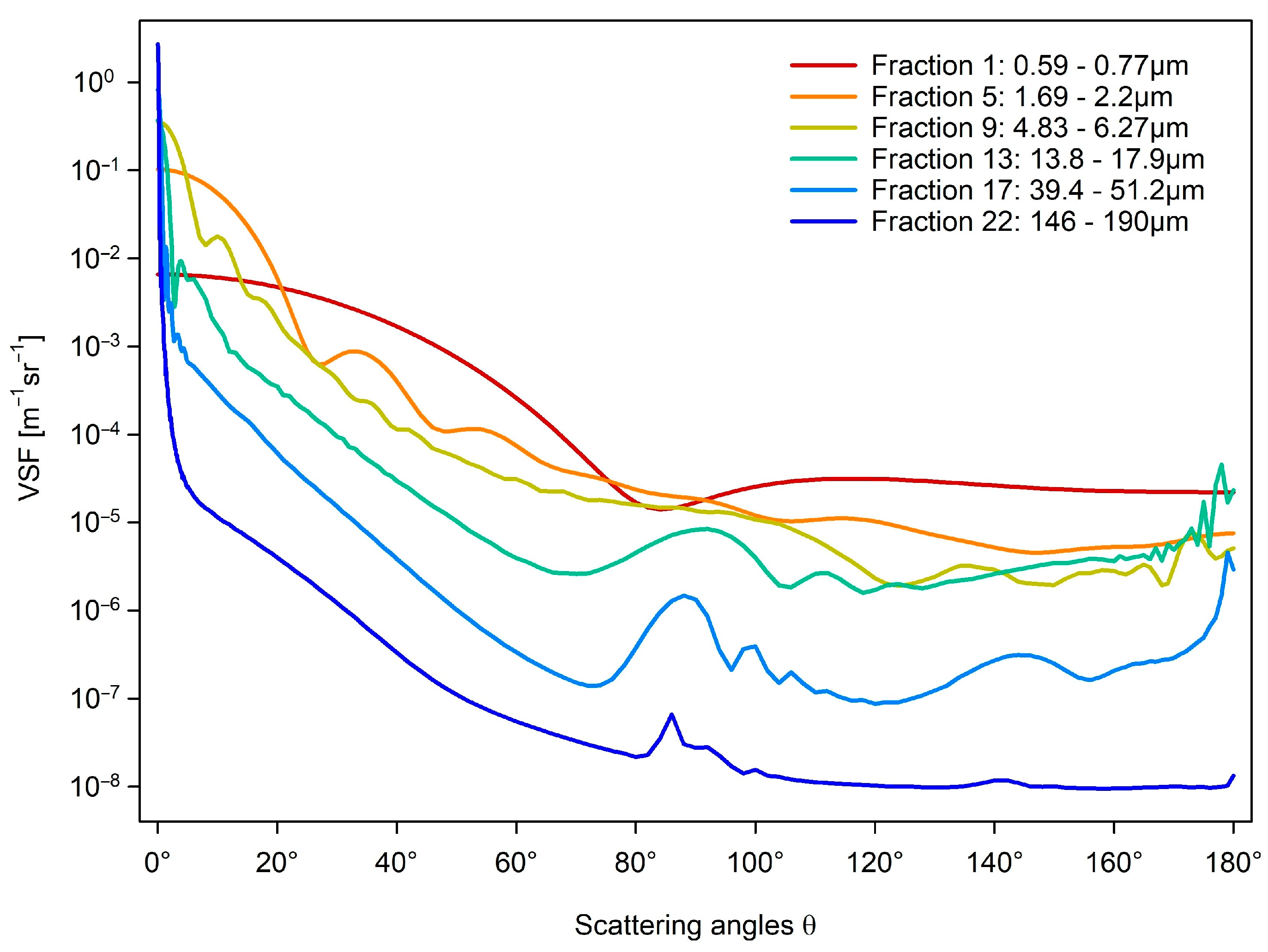
3.2. Scattering Coefficients and Volume Scattering Functions of Inorganic Suspensions

The computed scattering coefficients b_p for every size fraction of our model silica suspension are listed in the fourth column of Table 2 and shown in Figure 5a. The choice of geometric progression of the fraction boundaries caused every subsequent fraction to have an increasingly wider range of diameters and a decreasing concentration of particles, i.e., the number of particles in 1 m³ of suspension volume (see Table 2). These concentrations vary from 1.13 × 10¹¹ m⁻³ for the first fraction to 1.9 × 10³ m⁻³ for the last fraction, in which large particles have a diameter range of 0.146 to 0.19 mm. The total concentration of particles in all 22 fractions is 1.98 × 10¹¹ m⁻³, while the concentration sum of the first two fractions, which define the submicron particles in our distribution, is 1.62 × 10¹¹ m⁻³. Thus, the submicron particles account for more than 82% of the total number of particles. However, it is the micrometer-sized particles (represented by size fractions 3–11) that give the highest contribution to the scattering coefficient. The highest value of b_p = 1.74 × 10⁻² m⁻¹ is observed for fraction numbers 6 and 7, which have been assigned a range of diameters of 2.5 to 3.71 μm. This is the range of diameters that are 2.5 to over 4.2 times larger than the wavelength of the light that is scattered by these particles. In comparison, the b_p for the first particle fraction (the tiniest particles) is about 2.5 times lower and amounts to 7.16 × 10⁻³ m⁻¹, while for the last fraction (the largest particles), the b_p coefficient is 7.24 × 10⁻⁵ m⁻¹ and is over 240 times lower than the highest one. Submicron particles from size fractions 1–2 account for 13% of the total scattering coefficient of the model suspension, while micrometer-sized particles (fraction numbers 3–11) account for 82% of large particles (fraction numbers 12–22) for 5% of the total b_p.

The backscattering coefficient b_bp, defined by Equation (2), is shown for all 22 fractions in Figure 5b. It shows a monotonic decrease in value for increasing suspension particle size. The highest value of b_bp is 1.69 × 10⁻⁴ m⁻¹ and occurs for fraction number 1, while the lowest value is 8.12 × 10⁻⁸ m⁻¹ which is found for fraction number 22. The highest value is, thus, more than 2 thousand times larger than the lowest one.

The relative backscattering coefficient B_p, which is defined by Equation (3) is depicted in Figure 5c. Moving from the smallest particles towards the larger ones, the highest value is observed for fraction number 1, and it is 0.0236. Next, for fraction number 7, a local minimum is observed for which the B_p value is 0.0026. For subsequent fractions, the values increase up to fraction number 13, where the B_p is 0.0158. Further, it monotonically decreases and reaches the minimum value of 0.0011 for fraction number 22. The highest B_p value is, therefore, only 21 times greater than the lowest one.

For a better comparison, the calculated b_turb values are presented in Figure 5d and further described in the Discussion section.

Angular plots of the volume scattering functions are shown in Figure 6 for selected size fractions. The angular variability of the VSFs shows the typical dependence of these functions on particle sizes [38]. Large particles scatter light more asymmetrically than small particles, showing the domination of scattering into small forward angles. This will be shown in the examples of extreme fractions, i.e., fraction number 1 (particle diameters of 0.59–0.77 μm) and fraction number 22 (diameters of 146–190 μm). The VSF value for fraction number 22 reaches 1.62 m⁻¹sr⁻¹ at the scattering angle θ = 0.1°. At the same time, the lowest value of this function is 9.5 × 10⁻⁹ m⁻¹sr⁻¹ and it occurs for θ = 158°. The lowest value is, therefore, 171 million times smaller than the value for θ = 0.1°, which means that forward scattering is highly dominating. It is completely different for fraction number 1. Here, the VSF value at the angle θ = 0.1° is 6.61 × 10⁻³ m⁻¹sr⁻¹, while the lowest VSF value is 1.41 × 10⁻⁵ m⁻¹sr⁻¹ and it occurs for θ = 116°. The lowest value is, therefore, only 470 times smaller than the value for θ = 0.1°. This means that tiny particles contribute to backscattering more than others.

4. Discussion

Knowledge of the instrument’s weighting function allows us to link scattering-based measurements of suspended particles to their inherent optical properties, which is necessary in environmental science, particularly in oceanography [39]. Application of weighting functions improves the accuracy of models and algorithms that relate in situ measurements to data obtained through satellite remote sensing [40,41]. This study presents the application of the Seapoint turbidimeter’s weighting function in the correlation between turbidity signal and the scattering and backscattering coefficients at 880 nm for different sizes of suspended particles.

Since we had information about the VSFs for narrow-size fractions of the size distribution of the model inorganic suspension, the dependence of b_turb on the scattering properties was analyzed. Using Equation (3), the portion b_turb of the scattering coefficient b_p, measured by the turbidimeter, was calculated independently for each size fraction (see Figure 5d). The lowest value of b_turb is 1.53 × 10⁻⁷ and it was calculated based on the corresponding VSF function and γ function for fraction number 22. This is the fraction of the biggest particles, the diameters of which range from 146 to 190 µm. The highest value of b_turb is 4580 times greater and it is 4.72 × 10⁻⁴. It was obtained for fraction number 1. It is a fraction for which particle diameters are in a range of 0.59–0.77 µm.

Figure 7a presents the variability of the b_turb-to-b_p ratio for each of the 22 suspension fractions. The highest value of this ratio is observed for fraction number 1 and it is 0.066. The lowest value of the b_turb-to-b_p ratio of 0.0021 is observed for the largest fraction. This value is 31 times smaller than the highest one. The plot of b_p to b_turb (Figure 7b) shows no straightforward linear correlation. The determination coefficient r² here is 0.497.

The lack of correlation between b_turb and b_p did not satisfy the purpose of our study and led us to seek another stronger correlation. Since the angular shape of the weighting function points that 75% of the turbidity signal comes from angles higher than 90°, we analyzed the correlation of b_turb with the backscattering coefficient b_bp (defined by Equation (2)). The results are plotted in Figure 8. Figure 8a shows the change in the b_turb-to-b_bp ratio of all 22 fractions of the analyzed suspensions. The highest value of this ratio is 2.80 and it is observed for fraction number 2. It is a fraction for which particle diameters are in a range of 0.77–1 µm. The lowest value of b_turb-to-b_bp ratio is 0.93 and is observed for fraction number 14, for which diameters are in a range of 17.9 to 23.3 µm. The highest value is only three times higher than the lowest one. The correlation of b_bp-to-b_turb (see Figure 8b) shows a good linear relationship characterized by the determination coefficient r² of 0.979.

The correlation of b_bp-to-b_turb turned to be bi-modal in nature, therefore we also performed linearity analysis for two ranges of size fractions. Figure 8c shows fractions numbers 1–12, i.e., b_bp-to-b_turb correlation analysis for particles with diameters of less than 13.8 µm. Correspondingly, Figure 8d presents the correlation for particles larger than 13.8 µm. The r² determination coefficients are very high in both cases, 0.996 and 0.997, respectively. For all size fractions, the backscattering coefficient may be obtained as:

b_bp = 0.385·b_turb.

(8)

For the fractions smaller than 13.8 µm, more accurate relation will be

b_bp = 0.324·b_turb + 1.54 × 10⁻⁵,

(9)

while for the largest size fractions it will be:

b_bp = 0.991·b_turb.

(10)

Finally, we wanted to see how the b_turb signal correlates with the relative backscattering coefficient B_p (described by Equation (3)). Figure 9a includes an analysis of b_turb-to-B_p variability for all 22 size fractions. The highest values of this ratio were obtained for fraction number 6, i.e., for particles with diameters between 2.2 and 2.86 µm. Any smaller and larger particles gave lower values of the b_turb-to-B_p ratio. As with the correlation with b_p, Figure 9b shows a weak linear correlation between B_p and b_turb. The determination coefficient r² takes the value of 0.566, and the relationship could be attempted to be approximated by straight lines if as many as three particle size ranges were considered here.

The weighting functions of light scattering meters similar to the one given in Figure 3 have already been studied. As early as 1990, Oishi [42] proposed, based on calculations using the Mie solution, that the backscattering coefficient be determined by measuring the light scattering for an angle of 120°. This angle corresponds to the maximum of our γ(θ) function shown in Figure 3. A similar proposal was given by Ref. [43], who came up with the idea of placing a 700 nm illuminator and a detector in parallel to estimate the backscattering coefficient in natural waters. Their weighting function had a FWHM of only 20° and a maximum sensitivity at about 140°. This FWHM is 2.75 times lower than the Seapoint turbidity meter’s weighting function. The subsequent analysis [44] has led to the use of single-direction scattering correlation to determine b_bp in commercial instruments. These included HydroScat (former HOBI Labs Inc., Bellevue, WA, USA) and EcoBB (Sea-Bird Scientific, Bellevue, WA, USA). These meters gave information on the vertical profile of b_bp variability in in situ measurements when lowered to the bottom of a water body. Sullivan and Twardowski [45] proved that the variability of the VSF shape is the lowest for scattering angles between 110° and 120° and this angular range is, therefore, the best for b_bp estimation. For VSF measurements conducted in the Baltic Sea and oil-in-water emulsion droplets, a comparison of variability in this angle range was shown by Freda [46], who concluded that the VSF-to-b_bp correlation is free from angular variability for an angle of 117° as opposed to 140°. Also, observations have proved that the angular VSF shapes of ocean particles, normalized by b_bp, show low variability at angles close to 120° [47].

In our analysis we chose to test the correlation between turbidity signal and the scattering coefficients on inorganic particle suspension expecting that mineral particles will scatter near-infrared light (of 880 nm) in a similar way to the visible light [34,35]. However, in natural seawater, the infrared light is strongly absorbed in water. This is why there is a need to seek for further correlations between turbidity signal and backscattering coefficient in visible light range. We expect that there will be a satisfying correlation between turbidity signal and backscattering coefficients for selected visible wavebands. There are many recent studies on correlation of the remote sensing reflectance (derived for visible wavebands) with seawater turbidity on both global and regional scales [48], and most of the proposed algorithms base on a good relationship between water turbidity and reflectance signal. Remote sensing reflectance is one of the most important apparent optical properties, known to be related to the backscattering coefficient by a simple formula R_rs ~ b_b/(a + b_b) [49]. Garaba et al. [30] attempted to correlate turbidity measured at 700 nm with the mean remote sensing reflectance in the spectral range 630–660 nm achieving the linear fit of r² = 0.72. Dogliotti et al. [50] successfully correlated turbidity measured in the North Sea at 860 nm with the corresponding reflectance signal in the near-infrared region.

Application of turbidimeter weighting function in this study additionally showed that the correlation between the inherent optical properties and turbidity signal depends on particle size structure. The analyses presented in this paper naturally hypothesize that the results of turbidity measurements conducted with the Seapoint turbidimeter will be correlated with the backscattering coefficients in the visible light range, which is of most interest to opticians working in natural waters.

5. Conclusions

Turbidity measurements are commonly conducted in natural waters, providing information about the transparency of these waters. Such measurements are performed with a wide variety of instruments using different geometries of the measuring system. Thus, they give a turbidity result described in different scales, which cannot be converted into the inherent optical properties. This paper takes up the idea of correlating the Seapoint turbidimeter signal with the backscattering coefficient of the sample in an exemplary model of inorganic particle suspension.

In the first step, the angular weighting function of Seapoint turbidimeter was measured using a thin steel rod placed on a mobile stand in front of turbidimeter’s optical windows. Next, we created a model of silica suspension described by a typical power-law size distribution divided into 22 narrow-size fractions, from submicron to millimeter-sized particles. Then, we applied the turbidimeter weighting function to calculate the part of the scattering signal b_turb measured by the device. In the next step, the volume scattering functions were calculated for each size fraction and, thus, the IOPs of interest were obtained, i.e., b_b, b_bp, and B_p. The comparison with the calculated turbidity meter signal yielded the following conclusions:

• The weighting function of the Seapoint turbidimeter has the maximum sensitivity at an angle of 120°, which is consistent with many works [43,44,45,46] on single-angle scattering measurements for estimating the backscattering coefficient.
• This function has a high FWHM of 55° and 90% of the function falls in a wide range of scattering angles from 62° to 146°.
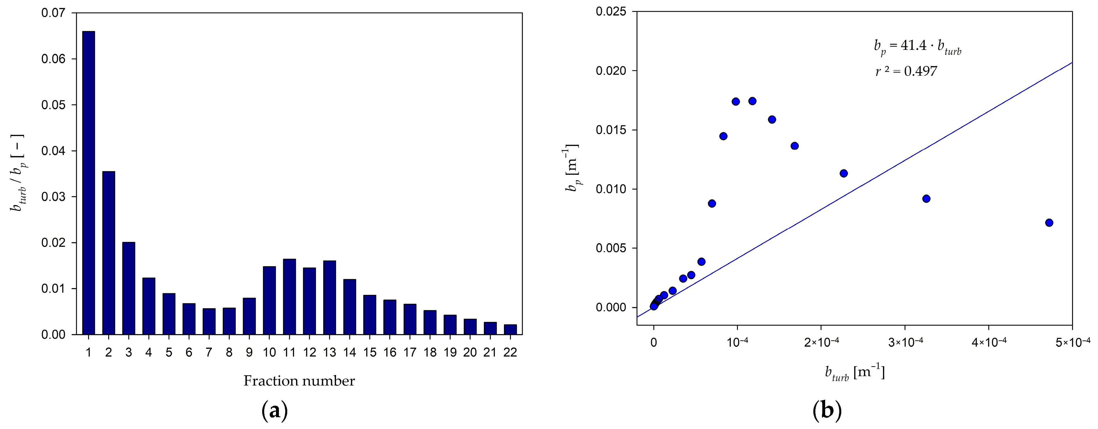
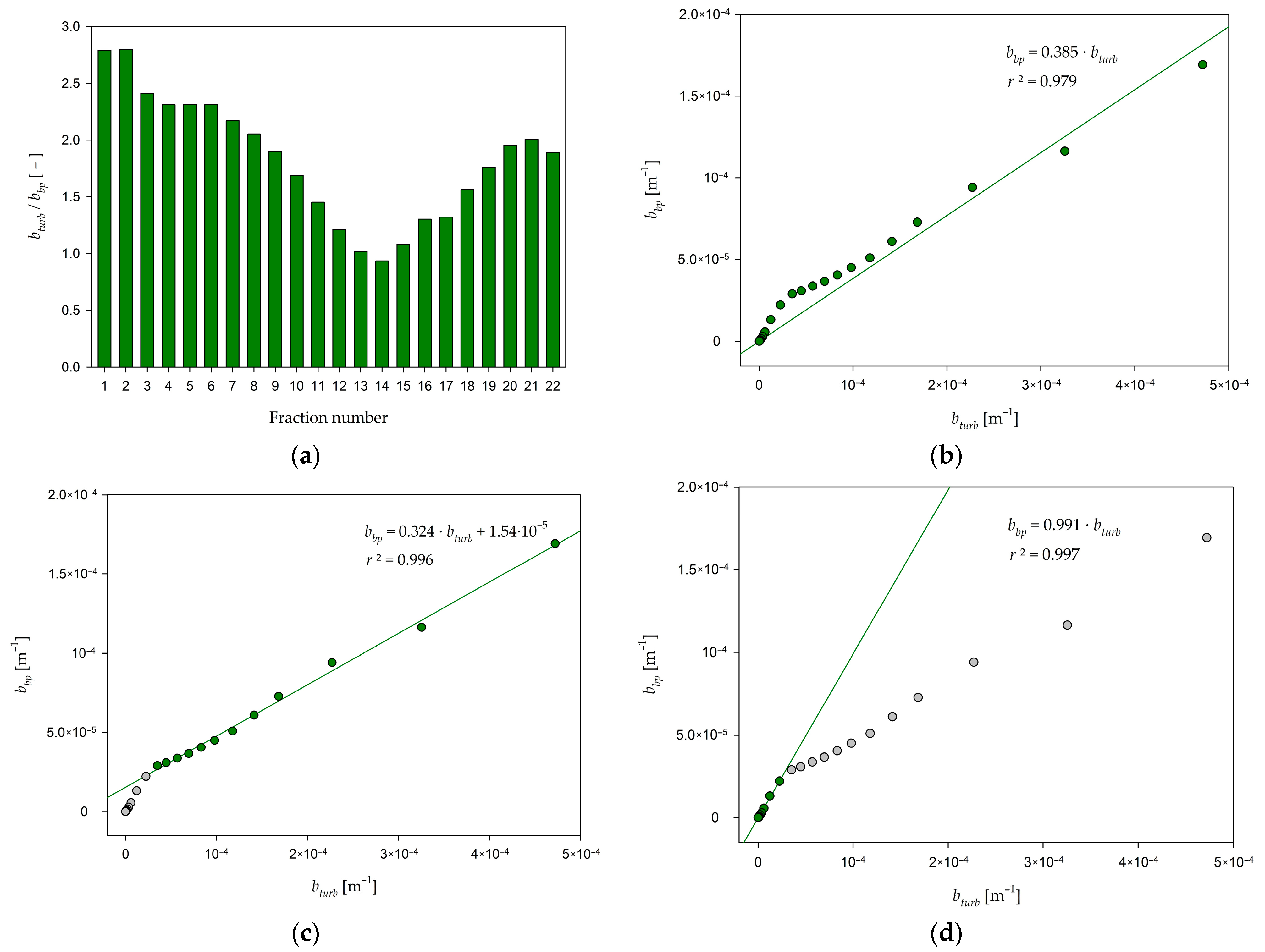
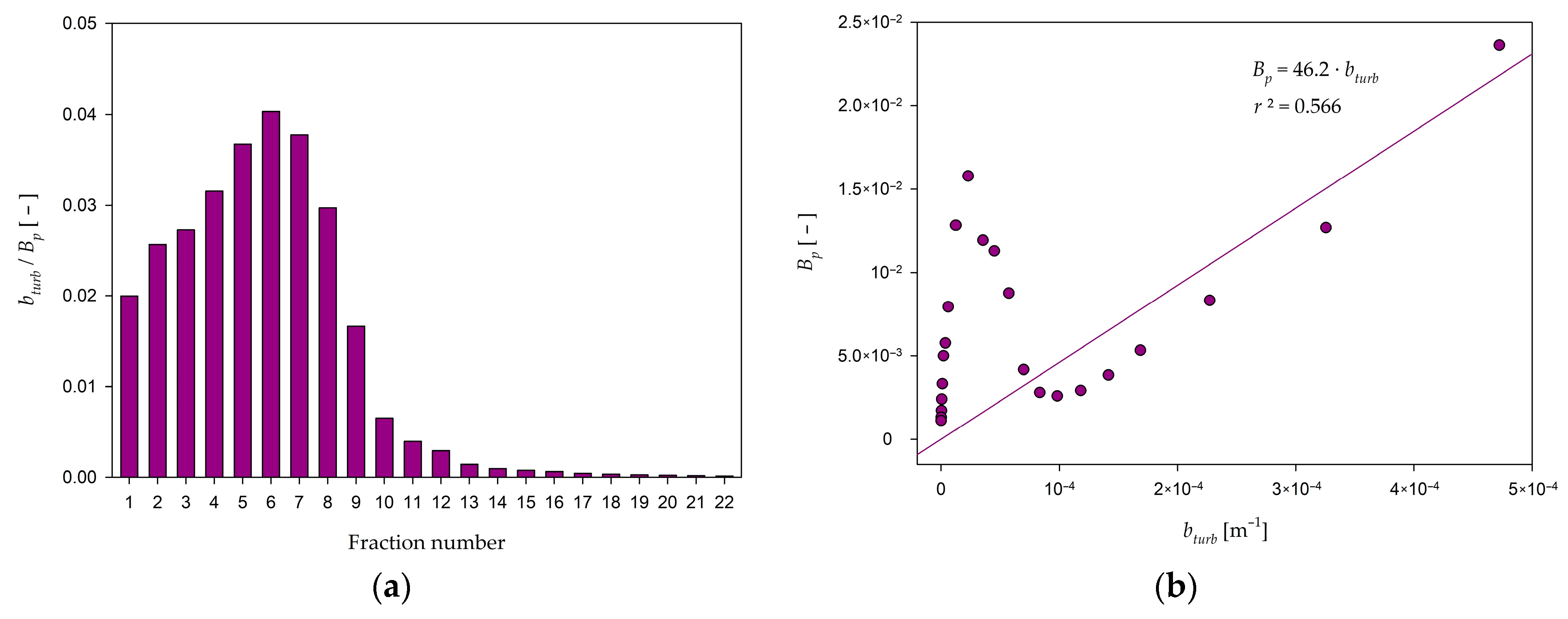
• Based on the modeling results, the turbidimeter signal has a good linear correlation with b_bp, but the best fit is obtained when we approximated b_bp separately for particles below 13.8 µm and particles larger than 13.8 µm.

Noteworthy is the fact that the light source for the Seapoint turbidimeter is a LED diode with a wavelength of 880 nm that is strongly absorbed in water. The next step will be to correlate b_bp (880) with other wavelengths in the visible range in a series of experiments performed under controlled conditions on different types of mineral and organic suspensions.

References

1. Directive 2000/60/EC of the European Parliament and of the Council of 23 October 2000 Establishing a Framework for Community Action in the Field of Water Policy. Available online: https://eur-lex.europa.eu/legal-content/EN/TXT/?uri=CELEX%3A02000L0060-20141120#E0039 (accessed on 18 December 2023).
2. Aas, E.; Høkedal, J.; Sørensen, K. Experiments with the Secchi disk. Ocean Sci. Discuss. 2013, 10, 1833–1893. [Google Scholar]
3. Tyler, J.E. The Secchi disc. Limnol. Oceanogr. 1968, 13, 1–6. [Google Scholar] [CrossRef]
4. Preisendorfer, R.W. American Society of Limnology and Oceanography Executive Secretary. Limnol. Oceanogr. 1989, 34, 1366. [Google Scholar]
5. Renk, H.; Nakonieczny, J.; Ochocki, S.; Lorenz, Z.; Majchrowski, R.; Ficek, D. Secchi depth-chlorophyll relationship in the Baltic. Acta Ichthyol. Piscat. 1991, 21, 203–211. [Google Scholar] [CrossRef]
6. Bright, C.E.; Mager, S.M.; Horton, S.L. Predicting suspended sediment concentration from nephelometric turbidity in organic-rich waters. River Res. Applic. 2018, 34, 640–648. [Google Scholar] [CrossRef]
7. Sadar, M. Making Sense of Turbidity Measurements—Advantages in Establishing Traceability between Measurements and Technology. In Proceedings of the 2004 National Monitoring Conference, Chattanooga, TN, USA, 17–20 May 2004. [Google Scholar]
8. Lednicka, B.; Kubacka, M.; Freda, W.; Haule, K.; Dembska, G.; Galer-Tatarowicz, K.; Pazikowska-Sapota, G. Water Turbidity and Suspended Particulate Matter Concentration at Dredged Material Dumping Sites in the Southern Baltic. Sensors 2022, 22, 8049. [Google Scholar] [CrossRef]
9. Dera, J. Marine Physics; PWN: Warsaw, Poland, 2003; pp. 1–514. [Google Scholar]
10. Pawlik, M.M.; Ficek, D. Validation of measurements of pine pollen grain concentrations in Baltic Sea waters. Oceanologia 2022, 64, 233–243. [Google Scholar] [CrossRef]
11. Pawlik, M.M.; Ficek, D. Spatial Distribution of Pine Pollen Grains Concentrations as a Source of Biologically Active Substances in Surface Waters of the Southern Baltic Sea. Water 2023, 15, 978. [Google Scholar] [CrossRef]
12. Constantin, S.; Doxaran, D.; Constantinescu, S. Estimation of water turbidity and analysis of its spatio-temporal variability in the Danube River plume (Black Sea) using MODIS satellite data. Cont. Shelf Res. 2016, 112, 14–30. [Google Scholar] [CrossRef]
13. Bin Omar, A.F.; Bin MatJafri, M.Z. Turbidimeter Design and Analysis: A Review on Optical Fiber Sensors for the Measurement of Water Turbidity. Sensors 2009, 9, 8311–8335. [Google Scholar] [CrossRef] [PubMed]
14. Haule, K.; Toczek, H.; Borzycka, K.; Darecki, M. Influence of Dispersed Oil on the Remote Sensing Reflectance—Field Experiment in the Baltic Sea. Sensors 2021, 21, 5733. [Google Scholar] [CrossRef] [PubMed]
15. Baszanowska, E.; Otremba, Z.; Piskozub, J. Modelling Remote Sensing Reflectance to Detect Dispersed Oil at Sea. Sensors 2020, 20, 863. [Google Scholar] [CrossRef]
16. Sadar, M. Turbidimeter Instrument Comparison: Low-Level Sample Measurement; Technical Information Series No. 7063; Hach Company: Loveland, CO, USA, 1999. [Google Scholar]
17. Anderson, C.W. Chapter A6. Section 6.7. Turbidity. In Techniques of Water-Resources Investigations 09-A6.7; Version 2.1; U.S. Geological Survey: Reston, VA, USA, 2005; pp. 1–55. [Google Scholar]
18. Haule, K.; Freda, W. Remote Sensing of Dispersed Oil Pollution in the Ocean—The Role of Chlorophyll Concentration. Sensors 2021, 21, 3387. [Google Scholar] [CrossRef] [PubMed]
19. Rymszewicz, A.; O’Sullivan, J.J.; Bruen, M.; Turner, J.N.; Lawler, D.M.; Conroy, E.; Kelly-Quinn, M. Measurement differences between turbidity instruments, and their implications for suspended sediment concentration and load calculations: A sensor inter-comparison study. J. Environ. Manag. 2017, 199, 99–108. [Google Scholar] [CrossRef] [PubMed]
20. Gray, J.R.; Gartner, J.W. Technological advances in suspended-sediment surrogate monitoring. Water Resour. Res. 2009, 45, 1–20. [Google Scholar] [CrossRef]
21. Gray, J.R.; Glysson, G.D. (Eds.) Proceedings of the Federal Interagency Workshop on Turbidity and Other Sediment Surrogates, Reno, Nevada, USA, 30 April 30–2 May 2002; Circular 1250; U.S. Geological Survey: Reston, VA, USA, 2003; pp. 1–56. [Google Scholar]
22. Merten, G.H.; Capel, P.D.; Minella, J.P.G. Effects of suspended sediment concentration and grain size on three optical turbidity sensors. J. Soils Sediments 2014, 14, 1235–1241. [Google Scholar] [CrossRef]
23. Trevathan, J.; Read, W.; Sattar, A. Implementation and Calibration of an IoT Light Attenuation Turbidity Sensor. Internet Things 2022, 19, 100576. [Google Scholar] [CrossRef]
24. EPA/600/R–93/100; Methods for the Determination of Inorganic Substances in Environmental Samples. U.S. Environmental Protection Agency: Cincinatti, OH, USA, 1993; pp. 1–178.
25. ISO 7027:1999(en); Water Quality—Determination of Turbidity. International Organization for Standardization: Geneva, Switzerland, 1999; pp. 1–10.
26. Gohin, F.; Bryère, P.; Lefebvre, A.; Sauriau, P.-G.; Savoye, N.; Vantrepotte, V.; Bozec, Y.; Cariou, T.; Conan, P.; Coudray, S.; et al. Satellite and In Situ Monitoring of Chl-a, Turbidity, and Total Suspended Matter in Coastal Waters: Experience of the Year 2017 along the French Coasts. J. Mar. Sci. Eng. 2020, 8, 665. [Google Scholar] [CrossRef]
27. Ouillon, S.; Douillet, P.; Andréfouët, S. Coupling satellite data with in situ measurements and numerical modeling to study fine suspended-sediment transport: A study for the lagoon of New Caledonia. Coral Reefs 2004, 23, 109–122. [Google Scholar]
28. Jafar-Sidik, M.; Gohin, F.; Bowers, D.; Howarth, J.; Hull, T. The relationship between suspended particulate matter and turbidity at a mooring station in a coastal environment: Consequences for satellite-derived products. Oceanologia 2017, 59, 365–378. [Google Scholar] [CrossRef]
29. Münzberg, M.; Hass, R.; Dinh Duc Khanh, N.; Reich, O. Limitations of turbidity process probes and formazine as their calibration standard. Anal. Bioanal. Chem. 2017, 409, 719–728. [Google Scholar] [CrossRef] [PubMed]
30. Garaba, S.P.; Badewien, T.H.; Braun, A.; Schulz, A.-C.; Zielinski, O. Using ocean colour remote sensing products to estimate turbidity at the Wadden Sea time series station Spiekeroog. J. Eur. Opt. Soc.—Rapid Publ. 2014, 9, 14020. [Google Scholar] [CrossRef]
31. Wang, Y.W.; Peng, Y.; Du, Z.; Lin, H.; Yu, Q. Calibrations of suspended sediment concentrations in high-turbidity waters using different in Situ optical instruments. Water 2020, 12, 3296. [Google Scholar] [CrossRef]
32. Mobley, C.D. Light and Water: Radiative Transfer in Natural Waters; Academic Press: Cambridge, MA, USA, 1994; pp. 1–592. [Google Scholar]
33. Mie, G. Beiträge zur Optik trüber Medien, speziell kolloidaler Metallösungen. Ann. Phys. 1908, 330, 377–445. [Google Scholar] [CrossRef]
34. Bohren, C.F.; Huffman, D.R. Absorption and Scattering of Light by Small Particles; John Wiley & Sons: Hoboken, NJ, USA, 1983; pp. 1–533. [Google Scholar]
35. Jonasz, M.; Fournier, G.R. Light Scattering by Particles in Water; Academic Press: Cambridge, MA, USA, 2007; pp. 1–714. [Google Scholar]
36. Available online: https://www.britannica.com/science/clay-mineral (accessed on 6 February 2024).
37. Rodríguez-de Marcos, L.V.; Larruquert, J.I.; Méndez, J.A.; Aznárez, J.A. Self-consistent optical constants of SiO2 and Ta2O5 films. Opt. Mater. Express 2016, 6, 3622–3637. [Google Scholar] [CrossRef]
38. Haule, K.; Freda, W. The effect of dispersed Petrobaltic oil droplet size on photosynthetically active radiation in marine environment. Environ. Sci. Pollut. Res. 2016, 23, 6506–6516. [Google Scholar] [CrossRef] [PubMed]
39. Santalices, D.; de Castro, A.J.; Briz, S. New Method to Calculate the Angular Weighting Function for a Scattering Instrument: Application to a Dust Sensor on Mars. Sensors 2022, 22, 9216. [Google Scholar] [CrossRef]
40. Heintzenberg, J.; Wiedensohler, A.; Tuch, T.; Covert, D.; Sheridan, P.; Ogren, J.; Gras, J.; Nessler, R.; Kleefeld, C.; Kalivitis, N.; et al. Intercomparisons and aerosol calibrations of 12 commercial integrating nephelometers of three manufacturers. J. Atmos. Ocean. Technol. 2006, 23, 902–914. [Google Scholar] [CrossRef]
41. McKee, D.; Piskozub, J.; Röttgers, R.; Reynolds, R.A. Evaluation and Improvement of an Iterative Scattering Correction Scheme for in situ Absorption and Attenuation Measurements. J. Atmos. Ocean. Technol. 2013, 30, 1527–1541. [Google Scholar] [CrossRef]
42. Oishi, T. Significant relationship between the backward scattering coefficient of sea water and the scatterance at 120°. Appl. Opt. 1990, 29, 4658–4665. [Google Scholar] [CrossRef]
43. Maffione, R.A.; Dana, D.R. Instruments and methods for measuring the backward-scattering coefficient of ocean waters. Appl. Opt. 1997, 36, 6057–6067. [Google Scholar] [CrossRef]
44. Boss, E.; Pegau, W.S. Relationship of light scattering at an angle in the backward direction to the backscattering coefficient. Appl. Opt. 2001, 40, 5503–5507. [Google Scholar] [CrossRef] [PubMed]
45. Sullivan, J.M.; Twardowski, M.S. Angular shape of the oceanic particulate volume scattering function in the backward direction. Appl. Opt. 2009, 48, 6811–6819. [Google Scholar] [CrossRef] [PubMed]
46. Freda, W. Spectral dependence of the correlation between the backscattering coefficient and the volume scattering function measured in the southern Baltic Sea. Oceanologia 2012, 54, 355–367. [Google Scholar] [CrossRef]
47. Zhang, X.; Boss, E.; Gray, D.J. Significance of scattering by oceanic particles at angles around 120 degree. Opt. Express 2014, 22, 31329–31336. [Google Scholar] [CrossRef] [PubMed]
48. Zheng, L.; Qiu, Z.; Zhou, Y.; Sun, D.; Wang, S.; Wu, W.; Perrie, W. Comparisons of algorithms to estimate water turbidity in the coastal areas of China. Int. J. Remote Sens. 2016, 37, 6165–6186. [Google Scholar] [CrossRef]
49. Gordon, H.R.; Brown, O.B.; Jacobs, M.M. Computed relationship between the inherent and apparent optical properties of a flat homogeneous ocean. Appl. Optics 1975, 14, 417–427. [Google Scholar] [CrossRef]
50. Dogliotti, A.I.; Ruddick, K.G.; Nechad, B.; Doxaran, D.; Knaeps, E. A single algorithm to retrieve turbidity from remotely-sensed data in all coastal and estuarine waters. Remote Sens. Envrion. 2015, 156, 157–168. [Google Scholar] [CrossRef]
Figure 1. The design of the test stand for measuring the angular weighting function of the turbidimeter.
Water 16 00594 g001
Figure 2. The spatial distribution of turbidity caused by light scattering from the rod placed in front of the turbidimeter in MilliQ water.
Water 16 00594 g002
Figure 3. Visualization of contribution to the turbidimeter signal from different scattering angles θ.
Water 16 00594 g003
Figure 4. The angular weighting function γ(θ) of the Seapoint turbidimeter.
Water 16 00594 g004
Figure 5. The simulated results of (a) the scattering coefficient bp, (b) the backscattering coefficient bbp and (c) the ratio Bp = bbp/bp for 22 size fractions of the model inorganic suspension. Graph (d) shows the values of bturb calculated using the turbidimeter’s weighting function for the same size fractions.
Water 16 00594 g005
Figure 6. The volume scattering functions of the model suspension of silica spherical particles for selected size fractions.
Water 16 00594 g006
Figure 7. The ratio of the calculated bturb of the turbidimeter to the scattering coefficient bp for each of the 22 size fractions of the model particle suspension (a) and linear correlation of bp to bturb (b).
Water 16 00594 g007
Figure 8. The ratio of the calculated bturb of the turbidimeter to the backscattering coefficient bbp for each of the 22 size fractions of the model particle suspension (a) and linear correlation of bbp-to-bturb (b). The correlation between bbp and bturb for fraction numbers 1–12 (c) as well as for fraction numbers 13–22 (d).
Water 16 00594 g008
Figure 9. The ratio of the calculated bturb of the turbidimeter to the backscattering ratio Bp for each of the 22 size fractions of the model particle suspension (a) and linear correlation of Bp to bturb (b).
Water 16 00594 g009