Article

Assessing Wet and Dry Periods Using Standardized Precipitation Index Fractal (SPIF) and Polygons: A Novel Approach

Engineering and Natural Sciences Faculty, Istanbul Medipol University, Beykoz, 34815 Istanbul, Turkey
Water 2024, 16(4), 592; https://doi.org/10.3390/w16040592
Submission received: 20 December 2023 / Revised: 11 January 2024 / Accepted: 14 February 2024 / Published: 17 February 2024

Abstract

:
In the open literature, there are numerous studies on the normal and extreme (flood and drought) behavior of wet and dry periods based on the understanding of the standard precipitation index (SPI), which provides a series of categorizations by considering the standard normal (Gaussian) probability distribution function (PDF). The numerical meaning of each categorization assessment is quite lacking in terms of future predictions of wet and dry period duration based on historical records. This paper presents a new approach for calculating possible formations of future wet and dry period durations based on historical records through an effective fractal geometric forecasting approach. The essence of the proposed methodology is based on the number of dry periods (steps) of non-overlapping monthly duration along consecutive broken line paths in the SPI classification for wet and dry period durations. It has been observed that the plot of periods on double logarithmic paper falls along a straight line against the number of such periods, implying a power function, which is the essence of fractal geometry. Extending the empirically derived straight line provides the number of periods that may occur in the future over a range of SPI levels. This methodology is referred to as SPI fractal (SPIF), and the classic SPI classification is converted into SPIF wet and dry polygons, which provide additional information about the drought period number within a valid polygonal area, compared to the classic SPI results. The wet and dry period features of any hydro-meteorology time series are constrained in SPIF polygons. The application of the methodology was carried out on monthly rainfall records on the European side of the Istanbul Florya meteorological station in Turkey.

1. Introduction

Global warming and its resulting impact in the form of climate change intensify the hydrological cycle to different extents in tropical, subtropical and polar climate zones. Global warming is a universal phenomenon in terms of temperature increase, but the most important meteorological factor in terms of climate change is the rainfall of temporal and spatial extreme values that cause the danger of floods and drought [1]. Although there are many methodological prediction processes for extreme events (floods and droughts), unfortunately, they have dangers that affect many aspects of social life [2,3,4,5,6,7,8,9]. Duration, magnitude, intensity, and temporal, spatial and better spatiotemporal distributions of droughts are important and each of them has a certain uncertainty even after the application of the best methodologies that are well known so far [10,11,12,13]. Drought is defined numerically and verbally by many standard indices such as the Palmar drought index (PDI) [14], standard precipitation index (SPI) [15], standard precipitation evapotranspiration index (SPEI) [16], stream flow drought index (SDI) [17] and others. The most interesting and widely used index is the SPI due to its simplicity and reliance on monthly rainfall records only. In some articles, it is referred to as the statistical standardization index, which is not correct. Its original proposal is based on the probabilistic standardization procedure that transforms the original probability distribution function (PDF) of a given monthly precipitation record into a standard normal (Gaussian) PDF with zero mean and unit standard deviation, as proposed by McKee et al. [15]. Traditionally, the probabilistic standardization approach has been used, but in this article, a new version of the SPI will be described as the SPI fractal (SPIF) version.
Recently, in terms of the multifractal SPI, another version of the SPI has been proposed by different authors and applied in different parts of the world [18,19,20,21,22]. There appears to be little information about the multifractal nature of precipitation indices [23]. SPI time series exhibit variable multifractal properties, with subdivisions having stronger persistence and multifractal properties for higher time scales [24]. On the other hand, multifractal analysis has also been used to analyze SPI series for different climatic zones of Nigeria at several temporal scales, and although the SPI was found to have multifractal properties, it did not show patterns across different climate descriptions [25]. The proposal of these authors is further developed by the fractal SPIF methodology, which provides a number of different wet and dry period forecasts and thus allows drought risk calculations to be made objectively.
The main aim of this paper is to present the intrinsic and serial features of standard precipitation index (SPI) behavior with fractal embedded features at different classification levels, which are useful for the verbal categorization of wet and dry periods in the past. The straight line properties of double logarithmic paper generally imply the fractal dimension in power function forms. In this paper, monthly rainfall records are illustrated with a fractal description between the succession of monthly wet and dry periods and their number. Extremely rainy and dry period durations are found probabilistically according to a certain risk level, but here, the fractal extreme values of the extremely rainy and especially dry (drought) periods are calculated as the number of single or consecutive events. In classical drought analysis studies, digital prime numbers are taken as the basis, regardless of the importance of fractal features in studies of drought quantities such as length (period), size and severity. However, the SPIF method relies on fractal features for a precise prediction approach. The application of theoretical explanations has been presented for the Florya/Istanbul meteorological records on the European side of Turkey for more than 60 years.

2. SPI and SPIF Methodologies

The basic concept of the standard precipitation index (SPI) was proposed by McKee et al. [15], and since then, there have been numerous studies, especially on the description of drought periods and comprehensive drought assessment studies. The first three columns of Table 1 give the classical SPI classifications. The last two columns are added as exceedance probability values of wet and dry period occurrences at each level. SPI classification can be obtained with the guidance of Table 1.
The SPI time series (SPI1, SPI2, …, SPIn) can be obtained from a certain n number of monthly precipitation time series (P1, P2, …, Pn) after completion of the flowchart steps in Figure 1.
The method of standardization for calculating the SPI has been adapted by many researchers as statistical standardization obtained by subtracting the mean value from each time series datum, and hence, the positive and negative deviations from the mean are obtained by the sum of deviations equal to zero. Finally, each deviation is divided by the standard deviation of the same time series, and this is considered standardization for the SPI application. This procedure is only valid if the original hydro-meteorology data fit the normal (Gaussian) probability distribution function (PDF). Otherwise, the probabilistic standardization procedure for the SPI basic concept applies. Implementation of the probabilistic standardization procedure can be accomplished using the following steps below.
(1)
Determine the probabilistic cumulative distribution function (CDF) that best fits the given hydro-meteorology record time series. In practical applications, the CDF of a given data set may fit one of the two- or three-parameter Gamma, Weibull, Log-normal, Log-logistic, Pearson, extreme value, etc., CDFs.
(2)
Calculate probability values pi (p1, p2, …, pn) from the CDF for each data value.
(3)
Convert these probability values to SPI1, SPI2, …, SPIn using the standard normal (Gaussian) CDF with zero mean and unit standard deviation.
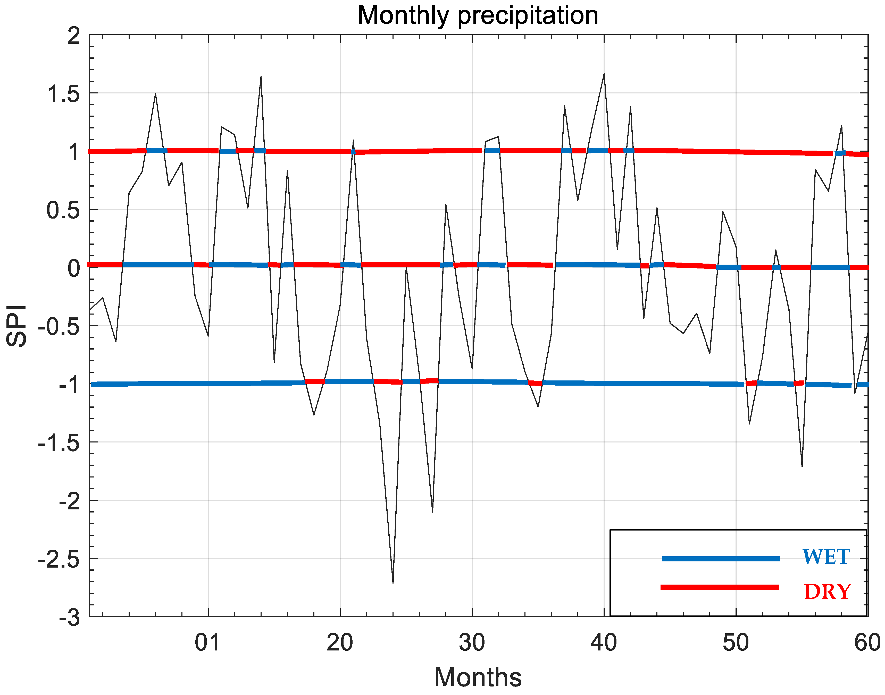
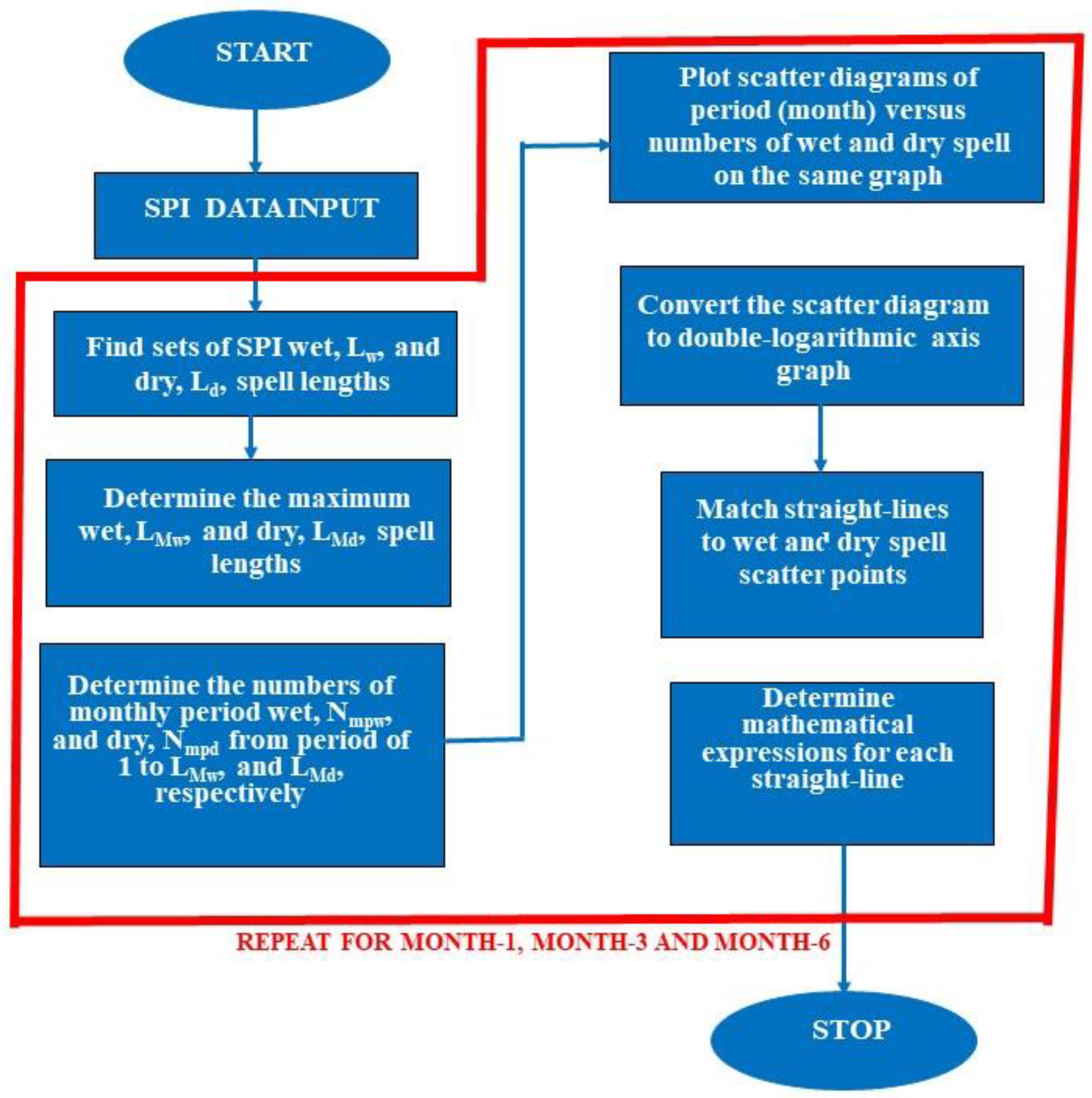
There are many geometric shapes that are similar, identical, repeated or randomly occurring called fractals [26]. Before entering the SPI fractal, classical SPI values are calculated in the slightly probabilistic standardization steps in the previous section. Thus, a representative time series for the SPI time series is given in Figure 2.
In this figure, alternating wet and dry spell sequences appear as broken (dashed) lines at any cut level. Throughout the SPI time series, the alternation of wet and dry periods is random in character, even if the wet period follows the dry period or vice versa. The number of wet and dry periods differ, but in a very long SPI time series, their number is practically equal. As mentioned in the introduction, there are many studies on the quality and quantity of the probabilistic and statistical characteristics of dry and wet periods. In this paper, an intermediate approach is adopted to investigate the wet and dry spell properties in an SPI in terms of fractals. The flowchart in Figure 3 presents the necessary steps for the successful application of the fractal procedure after the identification of the SPI time series as described in the previous section.
Any random sequence, for example, broken straight lines representing wet or dry periods, can be covered up to several sublengths, N(ri), where ri is the step length. With the number of steps, N(ri), the total length measured for any ri over a random succession of wet or dry periods, L(ri), can be expressed as follows:
L r i = r i N r i
In this equation, i represents the number of different step lengths. Since monthly precipitation records are taken into consideration in this paper, i is limited to the maximum dry length at a given SPI level, as shown in Figure 2. Therefore, the step lengths here are 1 month, 2 months, 3 months, …, n months, which do not overlap, and n is the maximum possible step length limited by maximum dry duration at the relevant SPI level.
Practically speaking, plotting the Ln[N(ri)] values against the Ln[L(ri)] values on double logarithmic paper appears as an inverted straight line, as shown in Figure 4.
The power function is the general mathematical representation of a straight line on a double logarithmic paper graph. The main meaning of an empirically derived straight line on a double logarithmic sheet is that the estimate of the number of wet and dry spells is spread over future periods. This figure implies that there is a power relationship between the relevant variables in the Cartesian coordinate system [26]. On the other hand, Minkowski (1864–1909) showed that if curve length is measured, for example, from a map of a certain scale, the measured length increases as the span of the compass (step length), r, decreases. The length, L(r), with a fractional compass’s aperture r, can be expressed empirically as follows:
L ( r ) = a N ( r ) m
where a is a constant and m is the slope of the straight line. This slope is related to fractional size. This last expression appears as a straight line on double logarithmic paper, as in Figure 4.
L n L r = l o g a + m L o g [ N ( r ) ]
Scale invariance of fractal geometries is one of the first concepts to be considered in the interpretation of any natural phenomenon. For example, according to the law of scale invariance, which determines the fractional size of lengths, frequency size distributions of various natural phenomena have been shown to have fractional sizes under various conditions. Ref. [26] used computer programming methods and fractional concepts to make synthetic replicates similar to real ones.
Although the precise definition of the concept of fraction is difficult, fractions can be easily understood by considering some simple geometric shapes, as in Figure 4, in their distinct fractional forms before moving on to their natural analogies with random fractions. As described above, the SPI provides wet and dry spell classification based on the magnitude of the standardized normal (Gaussian) PDF, whereas the SPIF, rather than classification, provides actual counts of possible wet and dry spell durations. The SPI provides time-series variation in wet and dry period classification after the conversion of the original data probability distribution function (PDF) to a standardized normal PDF with zero mean and unit standard deviation. The SPIF gives the actual number of wet and dry spells without any classification but gives its change by period. Additionally, the SPIF provides opportunities for future predictions by helping to determine the number of wet and dry periods over periods longer than the number of data points.

3. Application

The application of the SPI fractal proposal is presented for the monthly precipitation records of the Florya/Istanbul meteorological station on the European side of Turkey. According to the classification of Wladimir Köppen (1846–1940), the region is in the Csa class, with a Mediterranean climate and precipitation regime, where temperatures are above 20 °C in the hottest month and over 10 °C is possible for four months. Records are available over a long period of time, from 1940 to 2013. In the SPIF method application, monthly rainfall records are used as historical data. Changes in the data are highlighted fractally by double logarithmic (mathematical power function) calculations according to Equations (2) and (3). The application of the SPIF methodology to the Istanbul/Florya meteorological station provides predictions for future wet and dry precipitation occurrences in different periods, which cannot be obtained with the classical SPI approach.
Before any SPI calculation, it is necessary to know the original CDFs for a set of monthly precipitation data. Figure 5 shows three such CDFs for 1-month, 3-month and 6-month periods, all appearing in the form of Weibull CDFs.
In the continuation below, only 1-month fractal dimension calculations are presented, because the others are automatic repetitions of the same procedures. For this purpose, Figure 6 shows the classical SPI 1-month time series.
On first glance of this figure, the extremely wet (EW) periods at +2.00 have extreme rainy values of 8–9. On the other hand, dry extreme (ED) values are encountered very frequently at the extreme drought classification level. This shows that there has been a shift from wet periods to dry periods over 73 years. When preparing fractal graphs on double logarithmic paper, the following steps are necessary in light of the flowchart in Figure 3.
(1)
Divide each dry consecutive broken line profile into d1, d2, …, dn monthly periods and (step lengths) r1, r2, …, rn of non-overlapping parts of equal length, considering n ≪ int (maximum dry length).
(2)
Calculate the corresponding numbers, N(ri), of each step of all broken straight line dry periods as in the previous step.
(3)
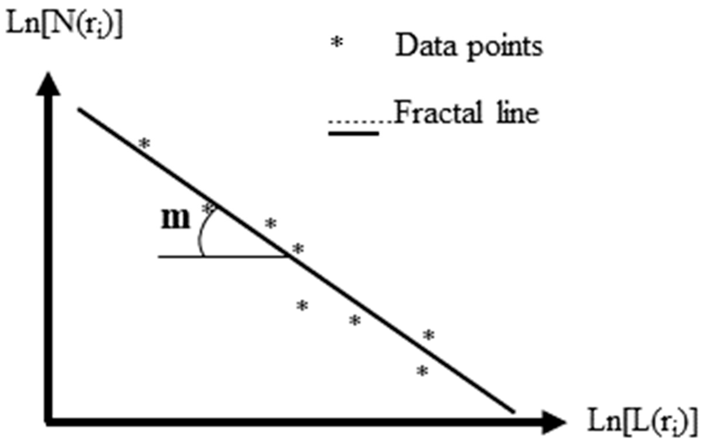
Plot the scatter diagram of each period (step length) against the corresponding N(ri) on double logarithmic paper.
(4)
Find the power function expression for each SPI level by placing the scatter points in a straight line on the double logarithmic paper.
(5)
Extend the best data match with a straight line on the horizontal period axis to 100 (102). This corresponds to the future prediction of the fractal relationship.
(6)
Draw the most interpretable inferences from the double logarithmic graphs collectively and individually, if necessary.
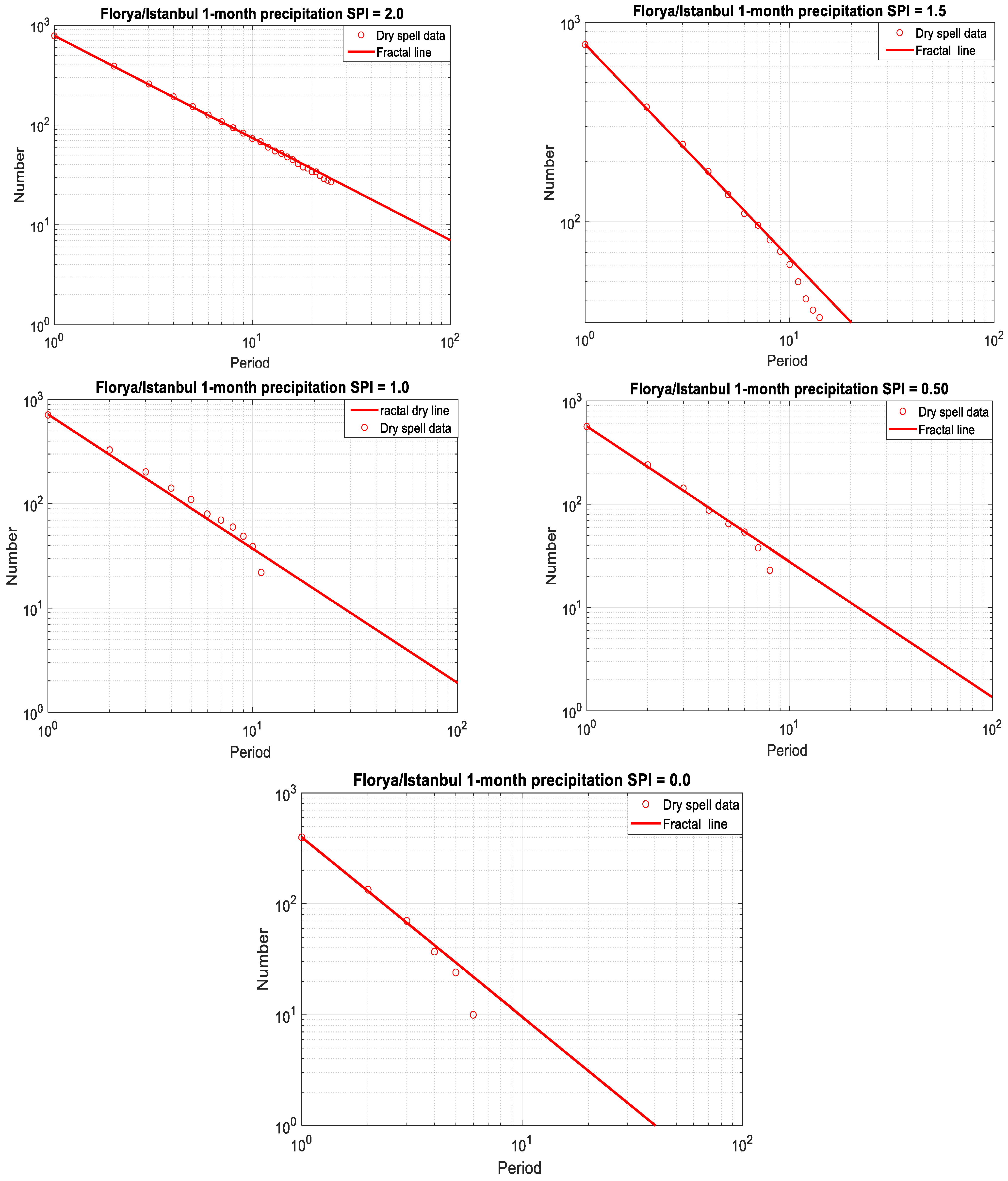
The application of the SPIF methodology to the Istanbul/Florya meteorological station provides predictions for future wet and dry precipitation occurrences in different periods, which cannot be obtained with the classical SPI approach. Figure 7 shows the fractal plots for straight lines in the form of scattering points for each SPI level of dry spell duration fractal dimension and the optimal power function parameters shown in Table 2 according to Equation (3). The lower and upper confidence levels are also shown in the same table.
The following interesting comments can be obtained from the fractal graphs in Figure 7.
(1)
Although dry spell lengths are random, they appear regularly along fractal straight lines in fractal graphs.
(2)
Logically, the steeper the slope of the line, the less likely the extreme value will occur.
(3)
The intersection of each straight line on the double logarithmic paper on the horizontal axis corresponding to NP = 1 gives the most extreme dry (drought) length that may occur in the future. These values can be calculated from the power function in Equation (3), considering the parameters a and m in Table 2.
(4)
All of the small and medium sample sizes fall along the double logarithmic straight line; this means that they are geometrically similar and thus have the property of self-similarity of fractal dimensions, as first proposed by Mandelbrot [27].
(5)
Dry straight lines are closer together at the SPI = 0.0 level but become farther apart as the level moves away from this level, but any two straight lines do not intersect each other. This means that dry period procedures have completely different climatological behavior.
(6)
The smaller the straight line slopes, the shorter and more persistent the dry duration appearances, which means dependence on long memory.

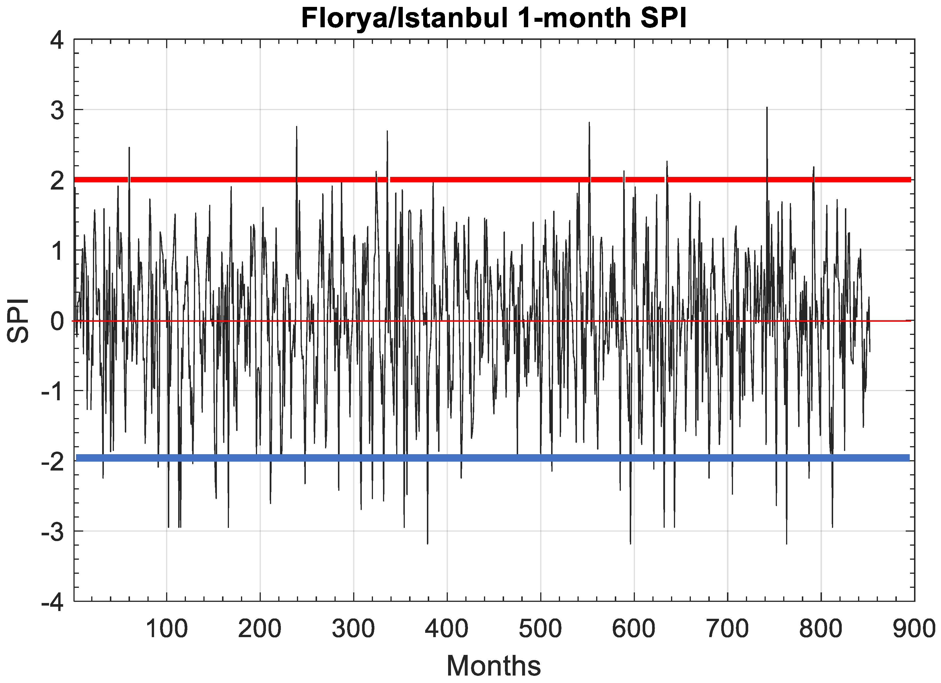
4. The SPIF Method for Dry Period Lengths
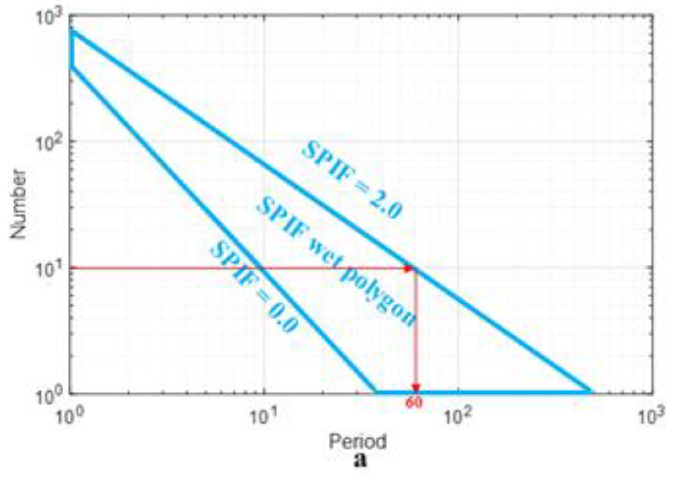
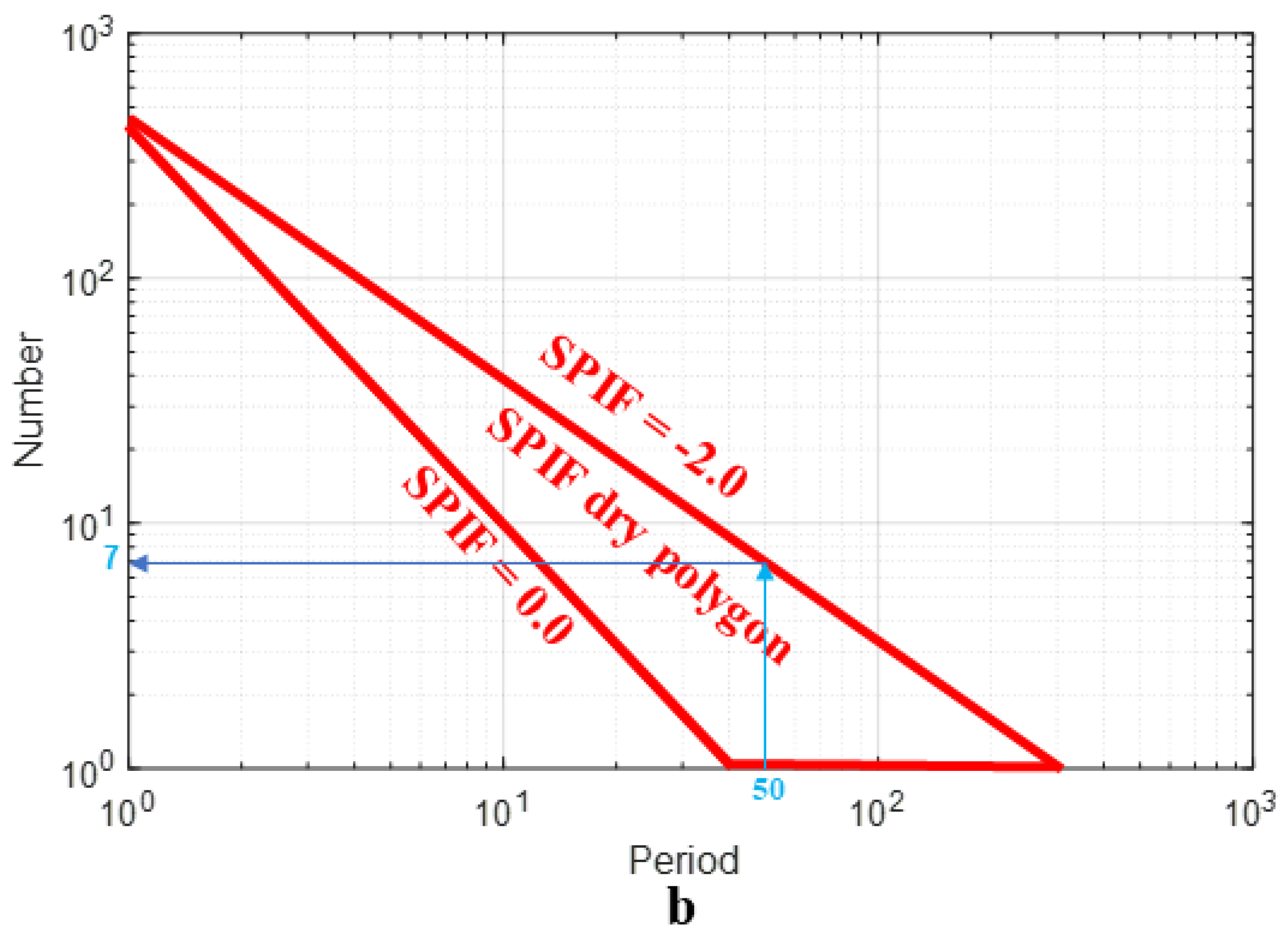
After determining the fractal parameters, as shown in Table 2, it is now possible to estimate the expectations for the dry period lengths of 1 month, 3 months, 6 months, 12 months, 24 months and 48 months. Decimal results are rounded to the next digital number.
In light of the SPI classifications in Table 1, it is possible to see that there are decreases (increases) from the highest (zero) categorization to the zero (lowest) level for wet (dry) periods. On the other hand, as the period duration increases, there are continuous decreases in the wet and dry periods.

5. SPIF Polygons

According to Table 1, wet (dry) SPI classifications are within the limits of SPI = 2.0 (−2.0) and SPI = 0.0. The generation of polygons in Figure 8 is based on numerical values in the graphs of Figure 7 and they are collected in Table 3; hence, the plot of wet and dry period durations against the number of occurrences of these periods can be drawn.
The following points are noteworthy for future SPI value predictions.
(1)
Since the number of 1-month wet and dry periods is very frequent in quadrangular polygons, there is a possibility that the number of wet and dry periods will decrease as the period increases.
(2)
All wet and dry spell period numbers are confined within the SPIF wet and SPIF dry polygonal area. These polygonal areas are areas where wet and dry spell behavior is suitable for Florya/Istanbul monthly rainfall events.
(3)
The lower limits of the SPIF = 0.0 in SPIF wet and SPIF dry polygon areas have the same common trend.
(4)
If one wants to know that such an event will occur 10 times, it is possible to know how many occurrences will correspond to a period of 1 month. Thus, in Figure 8a, the wet period can be entered on the vertical axis and the wet period on the horizontal axis can be found as 60 months. These numbers are substituted into Equation (3) with a and m parameters from Table 2, leading to a wet period of 12 months corresponding to SPIF = 2.
(5)
On the contrary, it can be found by entering a specific period, for example 50 months, on the horizontal axis of Figure 8b and then reading the corresponding number as 7 on the vertical axis. As in the previous step, one then substitutes these values into Equation (3).
There is no polygonal representation in the SPI approach, where only numerical values are categorized into a set of classes, as noted in Table 1. The polygonal SPIF representation provides the valid 2D relationship between the numbers of wet and dry periods and these periods, which cannot be obtained with the classic SIP method.

6. Discussion

In this paper, only short-term wet and dry period length characteristics are presented in detail in light of the classical SPI categorization for monthly rainfall records of more than 70 years in the Florya/Istanbul European-side meteorological station records. In general, extreme dry period exceedances appear to be higher than normal records. The classical SPI methodology does not provide additional information other than the classification shown in Table 2.
The difference between the classical SPI and the version proposed in this paper lies in SPIF, which is based on fractal dimensional feature definitions of wet and dry spell lengths.
A complete flowchart for classical SPI calculations based on the probabilistic standardization procedure is provided. Another flowchart for SPIF calculations based on the fractal dimensional procedure is also shown in detail. Although 1-month, 3-month and 6-month wet and dry period features are mentioned in the SPIF flowchart in this paper, the application is presented for a 1-month period, since the others have the same approach, and hence saving space is preferred. The following discussion points are noteworthy.
(1)
A new approach to the SPI procedure is presented by considering the number of consecutive, non-overlapping fixed scales (periods) of a series in a set of the classical SPI categorization levels.
(2)
This approach provides double logarithmic paper patterns as the basis for fractal dimension analysis, considering the number of wet and dry fixed periods in a given hydro-meteorology time series and the total length of these periods. This is not possible with the SPI procedure.
(3)
The double logarithmic graph of data extracted from a specific time series appears along a straight line, and its extension on the same graph provides the opportunity for future prediction. It should be noted that the number of extracted datum versus period length provides only a limited amount of data, and the extension line is a model for future similar, i.e., self-similar, data sets.
(4)
Knowing the number of a fixed period scale helps transfer these two variables to wet or dry period lengths through the power function, a key tool in fractal analysis.
(5)
All classical SPI classification results can be summarized in terms of wet and dry SPIF polygons. Therefore, the feasibility of wet and dry period classification can be determined.
(6)
Fractal charts help to determine the total expected durations of 1-month, 3-month, 6-month, 12-month, 24-month and 48-month wet and dry periods in a given monthly hydro-meteorology time series record.
(7)
Polygons help in finding the number of wet or dry periods given a fixed period, and these are then substituted into the fractal power equation, giving the total wet or dry period within the entire population of the given data set.

7. Conclusions

In this paper, it is emphasized and suggested that the standard precipitation index (SPI) approach is not based on statistical standardization but on the probabilistic standardization procedure that every researcher should follow for any standard drought index version in the literature. It is noted that although the correct application of the classical SPI provides a set of categorizations of the given hydro-meteorology time series, it does not provide predictions of future wet and dry periods. This paper reveals the fractal feature behavior of wet and dry period SPI values as a new approach called the SPI fractal (SPIF). The essence of this approach is based on the length of the wet and dry period versus the step length (period) that does not overlap with the wet and dry length, such as 1 month, along a series of broken (dashed) lines at any SPI categorization level. Thus, the scatter plots in the scatter diagram of the number of steps versus step length (period) appear along a straight line on the double logarithmic paper, modeled by a power function. The smaller the step length, the greater the number of spells, and so logically, there is an inverse relationship between the two variables. Extending this straight line on the double logarithmic paper until the number of step equals 1 provides future predictions that represent population behavior of the time series of interest. This procedure allows for the determination of wet and dry period lengths ranging from 1 month to multiple months. It is hoped that not only wet and dry period lengths but also intensity and frequency factors will be investigated fractionally for practical applications in the future. At the end of this study, wet and dry SPIF polygons that limit the wet and dry are obtained. The application of the SPIF procedure has been provided for monthly rainfall records of the Florya/Istanbul European-side meteorological station for more than 70 years.
The insight gained from the SPIF methodology is to estimate the actual number of wet and dry spell forecasts for a set of periods based on the fractal conceptual methodology. While the classical SPI approach helps in classifying wet and dry spells, the proposed SPIF methodology provides variation in the actual numbers based on past monthly rainfall records and helps in predicting future numbers of wet and dry spells through a straight line as representation of fractals on double logarithmic paper. The SPIF methodology can be used for water balance studies between wet and dry periods in real-world scenarios in the context of water resource management and for meteorological drought analysis in the context of meteorological applications. As for future research, the SPIF methodology can be extended not only to the number of wet and dry spells but also to their length, drought magnitude and intensity concepts.

Funding

This research received no external funding.

Data Availability Statement

The data are publicly available and will be forwarded to whoever requests.

Conflicts of Interest

The author declares that he has no known competing financial interests or personal relationships that could have appeared to influence the work reported in this paper.

References

  1. Chadwick, R.; Good, P.; Martin, G.; Rowell, D.P. Large rainfall changes consistently projected over substantial areas of tropical land. Nat. Clim. Chang. 2016, 6, 177–181. [Google Scholar] [CrossRef]
  2. Jaaskeläinen, J.; Veijalainen, N.; Syri, S.; Marttunen, M.; Zakeri, B. Energy security impacts of a severe drought on the future Finnish energy system. J. Env. Manag. 2018, 217, 542–554. [Google Scholar] [CrossRef] [PubMed]
  3. Stanke, C.; Kerac, M.; Prudhomme, C.; Medlock, J.; Murray, V. Health effects of drought: A systematic review of the evidence. PLoS Curr. 2013, 5. [Google Scholar] [CrossRef]
  4. Dominelli, L. Climate change: Social workers’ roles and contributions to policy debates and interventions. Int. J. Soc. Welf. 2011, 20, 430–438. [Google Scholar] [CrossRef]
  5. Oñate-Valdivieso, F.; Uchuari, V.; Oñate-Paladines, A. Large-scale climate variability patterns and drought: A case of study in South–America. Water Resour. Manag. 2020, 34, 2061–2079. [Google Scholar] [CrossRef]
  6. Tabari, H.; Hosseinzadehtalaei, P.; Thiery, W.; Willems, P. Amplified drought and flood risk under future socioeconomic and climatic change. Earth’s Future 2021, 9, e2021EF002295. [Google Scholar] [CrossRef]
  7. Bennett, B.; Leonard, M.; Deng, Y.; Westra, S. An empirical investigation into the effect of antecedent precipitation on flood volume. J. Hydrol. 2018, 567, 435–445. [Google Scholar] [CrossRef]
  8. Blauhut, V.; Stahl, K.; Stagge, J.H.; Tallaksen, L.M.; Stefano, L.D.; Vogt, J. Estimating drought risk across Europe from reported drought impacts, drought indices, and vulnerability factors. Hydrol. Earth Syst. Sci. 2016, 20, 2779–2800. [Google Scholar] [CrossRef]
  9. Lehner, F.; Coats, S.; Stocker, T.F.; Pendergrass, A.G.; Sanderson, B.M.; Raible, C.C.; Smerdon, J.E. Projected drought risk in 1.5C and 2C warmer climates. Geophys. Res. Lett. 2017, 44, 7419–7428. [Google Scholar] [CrossRef]
  10. Diffenbaugh, N.S.; Swain, D.L.; Touma, D. Anthropogenic warming has increased drought risk in California. Proc. Natl. Acad. Sci. USA 2015, 112, 3931–3936. [Google Scholar] [CrossRef]
  11. Naumann, G.; Alfieri, L.; Wyser, K.; Mentaschi, L.; Betts, R.A.; Carrao, H.; Spinoni, J.; Vogt, J.; Feyen, L. Global changes in drought conditions under different levels of warming. Geophys. Res. Lett. 2018, 45, 3285–3296. [Google Scholar] [CrossRef]
  12. Zhai, J.; Huang, J.; Su, B.; Cao, L.; Wang, Y.; Jiang, T.; Fischer, T. Intensity–area–duration analysis of droughts in China 1960–2013. Clim. Dyn. 2017, 48, 151–168. [Google Scholar] [CrossRef]
  13. Mishra, A.K.; Singh, V.P. A review of drought concepts. J. Hydrol. 2010, 391, 202–216. [Google Scholar] [CrossRef]
  14. Palmer, W.C. Keeping track of crop moisture conditions, nationwide: The new crop moisture index. Weatherwise 1968, 21, 156–161. [Google Scholar] [CrossRef]
  15. McKee, T.B.; Doesken, N.J.; Kleist, J. The relationship of drought frequency and duration to time scales. In Proceedings of the 8th Conference on Applied Climatology, Anaheim, CA, USA, 17–22 January 1993; Volume 17, pp. 179–183. [Google Scholar]
  16. Nalbantis, I.; Tsakiris, G. Assessment of hydrological drought revisited. Water Resour. Manag. 2009, 23, 881–897. [Google Scholar] [CrossRef]
  17. Vicente-Serrano, S.M.; Beguería, S.; López-Moreno, J.I. A multiscalar drought index sensitive to global warming: The standardized precipitation evapotranspiration index. J. Clim. 2010, 23, 1696–1718. [Google Scholar] [CrossRef]
  18. Kantelhardt, J.W.; Zschiegner, S.A.; Koscielny-Bunde, E.; Havlin, S.; Bunde, A.; Stanley, H.E. Multifractal detrended fluctuation analysis of nonstationary time series. Phys. A Stat. Mech. Appl. 2002, 316, 87–114. [Google Scholar] [CrossRef]
  19. García-Marín, A.P.; Estévez, J.; Medina-Cobo, M.T.; Ayuso-Muñoz, J.L. Delimiting homogeneous regions using the multifractal properties of validated rainfall data series. J. Hydrol. 2015, 529, 106–119. [Google Scholar] [CrossRef]
  20. Tan, X.; Gan, T.Y. Multifractality of Canadian precipitation and streamflow. Int. J. Climatol. 2017, 37, 1221–1236. [Google Scholar] [CrossRef]
  21. Yu, Z.G.; Leung, Y.; Chen, Y.D.; Zhang, Q.; Anh, V.; Zhou, Y. Multifractal analyses of daily rainfall time series in Pearl River basin of China. Phys. A Stat. Mech. Appl. 2014, 405, 193–202. [Google Scholar] [CrossRef]
  22. Adarsh, S.; Nourani, V.; Archana, D.S.; Dharan, D.S. Multifractal description of daily rainfall fields over India. J. Hydrol. 2020, 586, 124913. [Google Scholar] [CrossRef]
  23. Gómez-Gómez, J.; Carmona-Cabezas, R.; Sánchez-López, E.; de Ravé, E.G.; Jiménez-Hornero, F.J. Multifractal fluctuations of the precipitation in Spain (1960–2019). Chaos Solitons Fractals 2022, 157, 111909. [Google Scholar] [CrossRef]
  24. da Silva, S.A.; Stosic, T.; Arsenic, I.; Menezes, R.S.C.; Stosic, B. Multifractal analysis of standardized precipitation index in Northeast Brazil. Chaos Solitons Fractals 2023, 172, 113600. [Google Scholar] [CrossRef]
  25. Adarsh, S.; Kumar, D.N.; Deepthi, B.; Gayathri, G.; Aswathy, S.S.; Bhagyasree, S. Multifractal characterization of meteorological drought in India using detrended fluctuation analysis. Int. J. Climatol. 2019, 39, 4234–4255. [Google Scholar] [CrossRef]
  26. Ogunjo, S.T. Multifractal properties of meteorological drought at different time scales in a tropical location. Fluct. Noise Lett. 2021, 20, 2150007. [Google Scholar] [CrossRef]
  27. Mandelbrot, B.B. Fractal Geometry of Nature; WH freeman: San Francisco, CA, USA, 1982. [Google Scholar]
Figure 1. SPI calculation flowchart.
Water 16 00592 g001
Figure 2. Wet and dry periods.
Water 16 00592 g002
Figure 3. SPIF calculation steps.
Water 16 00592 g003
Figure 4. Illustrative fractional dimension calculations.
Water 16 00592 g004
Figure 5. CDFs for monthly periods.
Water 16 00592 g005
Figure 6. Florya/Istanbul 1-month SPI time series.
Water 16 00592 g006
Figure 7. FSPI graphs for the classical SPI as in Table 1.
Water 16 00592 g007aWater 16 00592 g007b
Figure 8. FSPI polygons for Florya/Istanbul 1-month precipitation. (a) Wet periods; (b) dry periods.
Water 16 00592 g008aWater 16 00592 g008b
Table 1. SPI classifications [15].
ClassStandard Class LimitsClassificationExceedance Probabilities
WetDry
1≥2Extremely wet (EW)0.0230.977
21.50–1.99Very wet (VW)0.0660.934
31.00–1.49Moderately wet (MW)0.1610.839
40.50–0.99Slightly wet (SW)0.3120.688
50.00–0.49Normal wet (NW)0.5000.500
60.00 to −0.49Normal dry (ND)0.6880.312
7−0.50 to −0.99Slightly dry (SD)0.8390.161
8−1.00 to −1.49Moderately dry (MD)0.9340.066
9−1.50 to −1.99Very dry (VD)0.9770.023
10≤−2Extremely dry (ED)0.9900.010
Table 2. Fractal parameters at different levels.
Florya/Istanbul Monthly Precipitation
SPI LevelsSpell Typea(with 95% Confidence Bounds)m(with 95% Confidence Bounds)
SPI-1 = 2Dry784.4(779.8, 789.1)−1.024(−1.031, −1.017)
WetNo dataNo dataNo dataNo data
SPI-1 = 1.5Dry779.3(768.1, 790.4)−1.074(−1.095, −1.053)
Wet50.0(48.96, 51.04)−3.634(−3.985, −3.282)
SPI-1 = 1.0Dry721.7(691.2, 752.2)−1.219(−1.288, −1.149)
Wet129.2(49.01, 209.4)−2.385(−6.474, 1.704)
SPI-1 = 0.5Dry569.2(548, 590.5)−1.309(−1.385, −1.233)
Wet277.4(257.2, 297.6)−1.755(−2.002, −1.508)
SPI-1 = 0.0Dry398.8(382.2, 415.4)−1.619(−1.747, −1.491)
Wet455.1(433.3, 476.8−1.519(−1.648, −1.391)
SPI-1 = −0.5Dry606.6(586.2, 626.9)−1.291(−1.358, −1.224)
Wet245.5(233.1, 257.9)−1.878(−2.075, −1.68)
SPI-1 = −1.0Dry712.8(692.7, 732.8)−1.183(−1.231, −1.136)
Wet139.2(65.61, 212.8)−2.317(−5.621, 0.988)
SPI-1 = −1.5Dry771.4(756.4, 786.3)−1.123(−1.153, −1.092)
Wet78.0No value−3.285No value
SPI-1 = −2.0Dry785.8(772.9, 798.6)−1.069(−1.09, −1.048)
WetNo dataNo dataNo dataNo data
Table 3. Wet and dry period features.
ClassStandard Class
Limits
Wet and Dry Period Durations
1 Month3 Months6 Months12 Months24 Months48 Months
1≥2784254125613015
21.50–1.99779239114542612
31.00–1.497221898135156
40.50–0.99569135542284
50.00–0.493997526931
60.00 to −0.496071476024104
7−0.50 to −0.997131948638177
8−1.00 to −1.49771225103472210
9−1.50 to −1.99786242116552613
10≤−2
Disclaimer/Publisher’s Note: The statements, opinions and data contained in all publications are solely those of the individual author(s) and contributor(s) and not of MDPI and/or the editor(s). MDPI and/or the editor(s) disclaim responsibility for any injury to people or property resulting from any ideas, methods, instructions or products referred to in the content.

