Article

Integrated Prediction Model for Upstream Reservoir Sedimentation in a Weir: A Comprehensive Analysis Using Numerical and Experimental Approaches

1
Department of Civil and Environmental Engineering, Incheon National University, Incheon 22012, Republic of Korea
2
Department of Safety Engineering, Incheon National University, Incheon 22012, Republic of Korea
*
Author to whom correspondence should be addressed.
Water 2024, 16(4), 574; https://doi.org/10.3390/w16040574
Submission received: 17 January 2024 / Revised: 12 February 2024 / Accepted: 13 February 2024 / Published: 15 February 2024

Abstract

:
In this study, a new empirical equation was established to predict the sedimentation volume resulting from the construction of a multi-purpose weir or low-head dam using experimental approaches. Applying the 1-D numerical model (STAFF), which is based on Exner’s equation, 2545 cases were simulated and laboratory experiments were conducted with various sediment particle sizes, channel slopes, inlet discharge, and outlet water elevation. Short-term predictions were conducted through laboratory experiments with movable bed, and the results indicated that dimensionless unit stream power and the Shields parameter exhibited the most significant correlation with dimensionless deposition volume. In particular, we analyzed the phenomenon in which the backwater effect and reservoir delta. Using a multiple regression approach, the developed empirical equation was validated for predicting sedimentation in the upstream reservoir of the weir.

1. Introduction

The dredging of river channels has been a common practice in the construction of low-head dams and multi-purpose weirs, where these hydraulic structures are designed to manage water flow and sediment movement patterns. However, such installations have led to significant alterations in the flow patterns of rivers and the transport of sediments. As a consequence, changes in sedimentation and erosion patterns within the river channel have become apparent. Over the medium to long term, this has resulted in modifications to the characteristics of the riverbed material, the cross-sectional shape of the river, and the slope of the riverbed. Furthermore, the management of water levels and flow control associated with multi-functional weirs have introduced an additional factor known as the backwater effect. This effect gradually gives rise to the formation of a reservoir delta. The reservoir delta is a distinct landform that emerges from the rapid deposition of sediment transported downstream, particularly in areas where water depths are higher, and flow velocities slow down due to the influence of hydraulic structures such as dams and weirs, which induce backwater conditions [1,2]. Reservoir deposition changes through a very complex process depending on sediment discharge generated from the river basin, transportation capacity, bed form, etc. In particular, it is primarily influenced by factors such as flood frequency, the topographical characteristics of reservoirs, operational strategies, cohesion capacity, density flow, and changes in land use. The analysis should consider various aspects, including the presence of dead zones, trap efficiency, the hydrograph of the upstream region, and sediment discharge [3]. The topographical features of a reservoir delta typically consist of three key elements: a topset bed composed of coarse pseudo-particles, a foreset bed forming a steep slope, and a bottomset bed characterized by silt or fine particles. The formation of this reservoir delta occurs when sediment-laden water from upstream meets the reservoir, causing a sharp reduction in flow velocity. This phenomenon results in a decrease in the effective storage capacity of the reservoir and an increase in the flood level of the river, thereby aggravating flood damages during the rainy season [3]. While, in the short term, a reservoir delta may not bring about significant topographical changes, its long-term effects can be substantial. These effects include a notable reduction in the cross-sectional area and storage capacity of the river, leading to issues such as the expansion of flood inundation and a decline in the reliability of stable water supply. Moreover, the sedimentation of reservoirs poses a threat to the safety of river embankments and hydraulic structures, impacting the operation and management of river facilities. Globally, it is well-documented that the storage capacity of dams decreases at an annual rate of approximately 0.5 to 1.0% due to sedimentation [4]. Additionally, Toniolo and Parker [5] have analyzed that the presence of reservoir deltas causes an annual decrease of about 1% in reservoir capacity [5].
In recent years, there has been a growing focus on issues related to reduced storage capacity due to sediment deposition and increased flood levels. Numerous researchers are actively investigating these challenges. Research into numerical modeling approaches for studying sediment deposition in natural rivers can be categorized based on the dimensionality of the numerical models employed. Among these approaches, 3-D numerical models are often employed to examine short-term variations in the movable bed, particularly in the vicinity of hydraulic structures such as piers, upstream of outfalls, and directly downstream of multi-purpose weirs. While these models are valuable for short-term predictions, conducting long-term predictions for relatively long-term periods demands substantial effort and time. To develop effective sediment management plans for areas upstream of weirs, it is imperative to comprehend the deposition mechanisms of reservoir deltas. Various empirical research methods and numerical analysis techniques have been employed to predict sediment deposition upstream of dams or reservoirs. Wright and Coleman [6] conducted field research along the Mississippi River in the United States, categorizing reservoir delta shapes into distal bars, bar backs, bar crests, and bar fronts.
Soni et al. [7], Hotchkiss [8], and Hotchkiss and Parker [9] conducted mathematical model experiments and numerical analyses to evaluate the applicability of one-dimensional numerical models for sediment transport. One-dimensional models for sediment transport provided an acceptable prediction for investigating bed elevation changes, offering insights into sediment transport processes over long-term durations [1,10,11,12]. Fan and Morris [13,14] analyzed data collected before and after flood events, as well as discharge-related data, with a focus on bed elevation changes in the Sanmenxia Reservoir within the Yellow River basin of China. Ahn et al. [15] utilized a one-dimensional model, GSTARS, to predict reservoir sedimentation and evaluate changes in riverbed conditions pre- and post-discharge events. This research collectively contributes to our understanding of sediment dynamics and hydraulic behavior in river systems. Choi [16] implemented laboratory experiments with mobile bed and validated empirical equations to predict sediment deposition.
Within the realm of sediment deposition in reservoirs, several experimental and field studies have provided valuable insights. In an experimental context, KanToush et al. [17] conducted hydraulic experiments and numerical analyses to investigate deposition in channels with rectangular cross-sections. Gökçen and Güney [18] carried out hydraulic experiments and subsequently applied previously established empirical equations to assess their impact on sediment transport, thoroughly analyzing the key influencing parameters. Matthieu et al. [19] developed an empirical equation by scrutinizing the relationship between reservoir deposition and critical parameters, including channel width, dimensionless length, and water depth, through hydraulic model experiments. Souza et al. [20] explored the prediction of deposition mechanisms via a combination of mathematical experiments and numerical analysis. Notably, there has been a growing expansion of numerical analysis studies in tandem with advancements in computing resources [21]. Moreover, efforts to enhance our understanding of the time series patterns associated with sediment transport mechanisms have been underway. This includes the application of neural network and machine learning technologies, as evidenced by the work of Latif et al. [22]. These endeavors collectively contribute to the ongoing refinement of our knowledge within the fields of river mechanics and hydraulics.
Sediment models are categorized based on application range (e.g., bed-material load vs. wash load, physical vs. chemical transport) and spatial/temporal formulation (e.g., 1D, 2D, 3D, steady vs. unsteady). Model selection depends on factors like problem scope, data availability, and time/budget constraints. While many models were developed for coarse sediments in rivers, reservoirs present challenges due to diverse grain sizes and cohesive sediments. Reservoirs are typically depositional, but erosion can occur during drawdown. Sediment-laden inflows disrupt equilibrium, and cohesive sediments vary in erodibility. Inflow and flushing entail a mix of grain sizes. Complex delta geometry affects erosion. Reservoir sediment transport is complex, exceeding current analysis capabilities, warranting caution in numerical techniques [12].
The primary objective of this research is to investigate the volume and spatial distribution of sediment deposition upstream of a weir through experimental studies. The study aims to examine the relationship among key parameters such as sediment particle size, bed slope, flow velocity, and water depth, which interactively influence sediment deposition mechanism. To achieve this goal, a one-dimensional numerical analysis model was employed to analyze these parameters, ultimately leading to the derivation of an empirical equation for predicting sediment deposition volume. The developed equation was rigorously tested and validated against experimental results to ensure its accuracy and reliability.

2. Theoretical Backgrounds

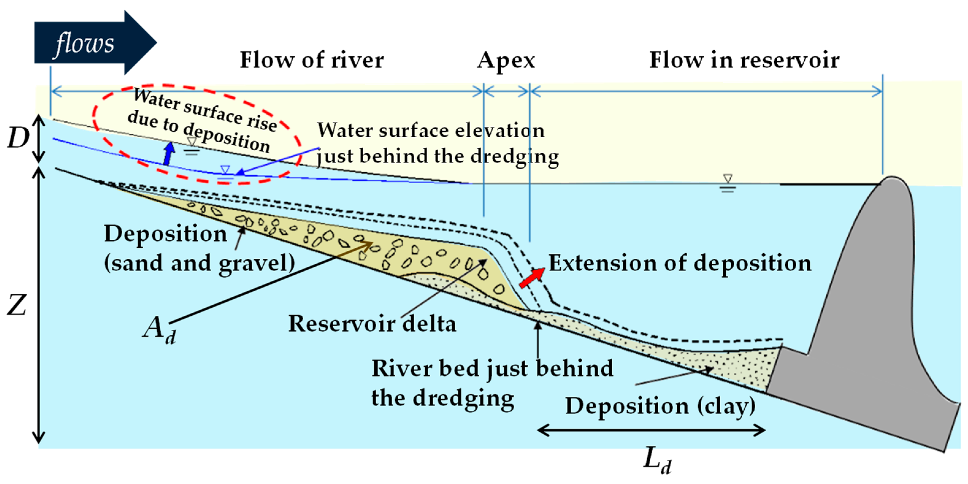
2.1. Reservoir Delta Theory

Backwater forms in reservoirs located upstream of hydraulic structures, such as dams or multi-purpose weirs, which serve various functions like flood control and water supply. When the flow entering into this backwater section increases, it results in an expansion of the passage area and a subsequent decrease in flow velocity and turbulence. Consequently, the sediment transport capacity decreases, causing sediments from upstream to settle at the reservoir’s bottom. In this process, coarser sediments, such as gravel and sand, tend to preferentially deposit at the reservoir inlet, gradually forming what is known as a reservoir delta. On the other hand, fine particles like silt and clay pass through the reservoir delta in the form of density flow and subsequently settle within the reservoir. It is worth noting that if the inflowing sand from the basin contains a significant proportion of fine particles, the impact of fine particle deposition due to density currents on the reduction of reservoir capacity may not be substantial.
Sediment deposition within the reservoir occurs gradually over a specific period during the operation of a weir or dam. As the river’s flow diminishes, coarse materials accumulate in the impounded water, primarily in the upstream section of the reservoir. The transportation of bed load is driven by the movement of water waves. In this study, the concept of a reservoir delta, as depicted in Figure 1, is introduced to analyze the behavior of the reservoir delta upstream of the weir in response to the presence of a multi-purpose weir [23].
Variables in Figure 1 are defined as follows: Ad represents the sediment load amount per unit width, and Ld indicates the distance from the main body of the multi-purpose weir to the starting point of the reservoir delta. To analyze the behavior of sediment particle erosion and deposition, dimensionless variables were introduced, as illustrated in Figure 2.
In Figure 2, the concept of VS/ω is an extension of VS (Unit Stream Power), originally proposed by Yang [24]. It represents the rate of energy dissipation of water per unit weight divided by the fall velocity (ω) of sediment particle. And V and S denote the flow velocity and the riverbed slope, respectively. U*/ω represents the ratio of the friction velocity applied to sediment particles and the fall velocity acting in the direction of gravity, and the delivery and deposition of sediment particle can be determined according to U*/ω.
U * = g R S
τ * = τ 0 γ ( G 1 ) d s
where U* = the friction velocity (m/s); g = gravitational acceleration (=9.81 m/s2); R = hydraulic radius (m/s); τ* = the Shields parameter (−); τ0 = bed shear stress (N/m2); γ = specific weight of water (N/m3); G = specific gravity of sediment (−); and ds = sediment particle size (m). It should be noted that the Shields parameter can be calculated based on particle size and unit weight of sediment, and the shear velocity of the particle, as previously defined by Shields [25]. The Shields parameter is utilized in the analysis of incipient motion criteria for sediment particles and the assessment of changes in riverbed morphology. It is defined in Equation (2) as a dimensionless variable that corresponds to the vertical axis of the Shields diagram.
This study primarily focuses on the computation of one-dimensional sedimentation patterns and sediment deposition amounts (Ad) to examine the sedimentation pattern of a reservoir delta. To achieve this, a combination of numerical analysis using a one-dimensional numerical model and mobile bed experiments was conducted. The objective was to reveal relationships between dimensionless deposition per unit width (Ad/qt) and dimensionless variables such as dimensionless unit stream power (=VS/ω), the Shields parameter (=τ*), and U*/ω. The aim was to investigate and comprehend these relationships thoroughly.

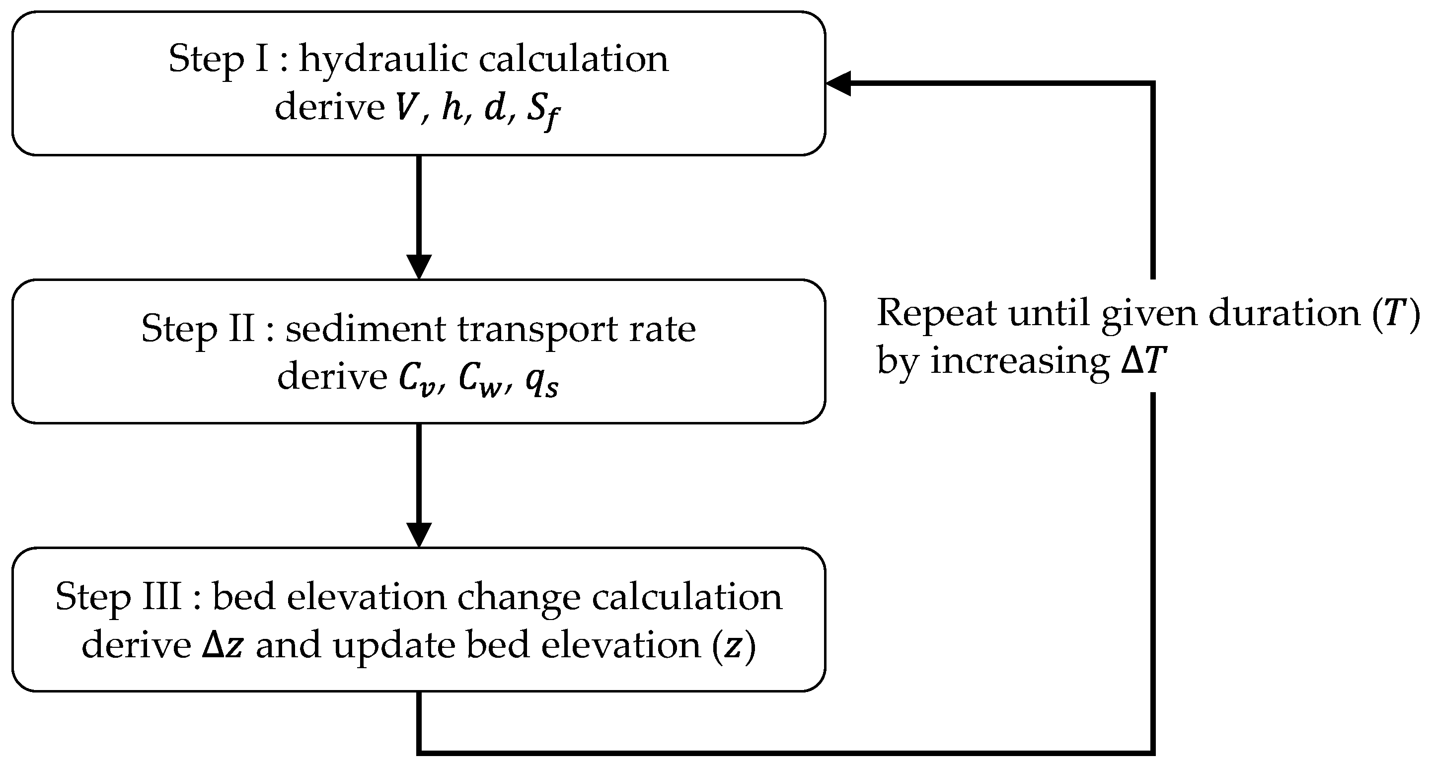
2.2. Model Description

HEC-RAS, GSTARS, SRH-2D, and Delft3D, which are widely utilized one-dimensional numerical simulation for bed elevation change and sediment transport modeling, employ an un-coupled scheme [10,26,27,28]. This scheme calculates hydraulics and sediment routing processes separately. The numerical analysis technique utilized in this study also employs the uncoupled scheme akin to a standard one-dimensional bed elevation change model. The process commences with hydraulic analysis, which uses defined upstream and downstream boundary conditions to compute hydraulic parameters such as flow velocity, water depth, bottom shear stress, and friction slope. Subsequently, these hydraulic parameters are employed to calculate sediment transport. Finally, bed elevation change can be calculated. The bed elevation change is then updated, and the model progresses to the next time step, repeating the same sequence of calculations. These approaches are referred to as the STAFF (Sediment Transport Analysis For Flume) model, and its detailed descriptions are given as follows.
  • Flow velocity
Using the energy equation given as follows:
h 2 + β 2 V 2 2 2 g = h 1 + β 2 V 1 2 2 g + h L
where subscripts 1 and 2 denote the downstream and upstream, respectively; h = water surface elevation (m); β = energy coefficient (≈1); and hL = energy loss (m). Assuming that hL is initiated by bottom friction, it can be expressed as the arithmetic average of the upper and lower cross sections as follows:
h L = 1 2 S f 2 + S f 1 Δ x
where Sf = friction slope (−); and Δx = stream-wise distance (m). Equation (4) can be rewritten with Equation (3) as:
h 2 = h 1 + V 1 2 2 g V 2 2 2 g + 1 2 S f 2 + S f 1 Δ x
Since this study focused on simulating the stream- and depth-wise direction behavior of a rectangular cross-section, the following relationship can be satisfied.
V 2 2 2 g = q 2 2 g d 2 2 = q 2 2 2 g h 2 Z 2 2
V 1 2 2 g = q 2 2 g d 1 2 = q 1 2 2 g h 1 Z 1 2
where q = discharge per unit width (m2/s); d = water depth (m); and Z = bed elevation from datum (m). Using Manning’s roughness equation:
S f 2 = n 2 q 2 h 2 Z 2 10 3
S f 1 = n 2 q 2 h 1 Z 1 10 3
where n = the Manning’s roughness coefficient. Substituting Equations (6)–(9) into Equation (5) yields
f h 2 = h 2 h 1 q 1 2 2 g h 1 Z 1 2 + q 2 2 2 g h 2 Z 2 2 1 2 n 2 q 2 h 2 Z 2 10 / 3 + n 2 q 2 h 1 Z 1 10 / 3 Δ x = 0
The STAFF model calculates h2 using the Newton-Raphson method when h1 is given.
2.
Sediment load
In this study, sediment concentration was calculated using the Engelund–Hansen formula [29]. According to previous studies, the Engelund–Hansen equation, being dimensionless, is considered the most suitable for sand transport computation, offering advantages in its application [30,31].
C w = 0.05 G G 1 V S f G 1 g d s 1 / 2 d S f G 1 d s 1 / 2
where Cw = sediment concentration by weight (−). Cv (=sediment concentration by volume, g/l) can be rewritten as follows:
C v = C w G G 1 C w
Also, sediment discharge per unit width, qs, can be calculated as follows:
q s = C v · V · d s
3.
Bed elevation change
Research on predicting bed elevation change according to the flow of water in natural rivers began when Exner [32] first introduced the continuity equation with the concept that the mass of water and sediment is conserved. Notably and recently, Dodaro et al. [33] conducted a remarkable experimental study exploring a modified Einstein sediment transport method for analyzing local scour patterns downstream of a rigid bed, which stands as a representative and highly relevant recent study. In particular, their investigation of non-uniform flow conditions through laboratory experiments and numerical simulations offers insights into turbulent flow dynamics and bed material properties pertinent to our discussion. Assuming one-dimensional flow in which the riverbed moves and there is no lateral inflow, the Exner equation can be rewritten as follows:
( 1 p ) Z t = q s x
where p = porosity of soil (−); t = time (sec.); and x = stream-wise length (m). Differencing Equation (14) with FTBS (Forward in Time Backward in Space) scheme:
Δ Z j k = Z j k + 1 Z j k = 1 1 p q s j k q s j 1 k · Δ t Δ x
where ΔZ = bed elevation change (m); Δt = time step (sec.); and j and k = spatial and temporal index. The calculation procedure (hydraulic variables for steady flow, sediment load, bed elevation change) described in Figure 3.

3. Laboratory Experiments

3.1. Dimensional Analysis

Dimensional analysis was performed to analyze the factors affecting the sedimentation amount. Representative factors affecting Ad are as follows:
A d = f ( ρ ,   ν ,   H ,   D ,   S ,   d s ,   ω ,   g ,   V ,   U * ,   t ,   C u )
where ρ = density of fluid (kg/m3); ν = kinematic viscosity (m2/sec.); D = upstream normal depth (m); and Cu = sediment non-uniformity constant (−). Rewriting Equation (16) for performing the standard dimensional analysis:
A d q t = f ( R e ,   Fr , R e * , ω t D ,   D d s , V S ω , U * ω , τ * , H D )
As the experimental flow and movable bed condition in this study represented the fully turbulent flow with a single size of particles, the sensitivity analysis was performed on the remaining six dimensionless parameters excluding Re, Re*, Fr, and Cu.

3.2. Model Similarity

River hydraulics research can be categorized into two main types: (1) researches focusing on water level and flow rate within the channel; and (2) researches concentrating on sediment transport and bed elevation changes. The former typically employs a fixed bed model, while the latter involves a mobile bed model. When conducting hydraulic model experiments using a scaled-down model to understand the hydraulic behavior occurring in natural rivers, as is the case in this study, it is essential to ensure hydraulic similitude between the flow behavior in the prototype and the scaled model. Generally, in hydraulic experiments, Froude similitude and Reynolds similitude are the primary similitudes applied. However, in mobile bed experiments, achieving ideal conditions for these variables can be challenging due to issues such as spatial constraints and limitations in implementing sediment particles. Consequently, in this study, experimental conditions were devised to meet the similitude for sediment discharge by applying the Exner equation, which served as the governing equation for the analysis of bed elevation changes.
Equation (14) can be expressed as follows:
Δ Z = 1 1 p Δ q s Δ x Δ t
To satisfy hydraulic similitude, Equation (18) can also be expressed with conversion ratio between prototype and scaled model as follows:
t r = 1 p r X r Z r q s r 1
where subscript sr = scale ratio between prototype and scaled model; Xr, and Zr = scale ratios for horizontal and vertical direction, respectively; and qsr = scale ratio of sediment load per unit width. qsr in Equation (19) can be calculated through the scale ratio of qsp and qsm as follows. Sediment load per unit width can be calculated using the sediment transport formula proposed by Yang [34]. It was assumed that the amount of sediment in a river is related to the dissipation rate of the potential energy of water, and if the potential energy of a river decreases by Δz at Δt, its dissipation rate is as follows:
Δ z Δ t = Δ x Δ t Δ z Δ x = V S
In this context, Yang [34] introduced the concept of unit stream power, defining it as the power of water per unit weight. He developed an equation using existing sediment transport data with unit stream power as a variable, which is as follows:
l o g C t = 5.435 0.286 l o g ω d s ν 0.457 l o g U * ω + 1.799 0.409 l o g ω d s ν 0.314 l o g U * ω × l o g V S ω V c S ω
where Ct = sediment concentration in parts per million by weight (ppm); Vc =critical average flow velocity in incipient motion, m/s, and can be calculated with following Equation (22):
V c ω = 2.5 l o g U * d s / ν 0.06 + 0.66 ; 1.2 < U * d s ν < 70 2.05 ; U * d s ν 70
The procedure to estimate total sediment load using Yang’s formula [34] is as follows:
-
Estimate VS, ωds/ν, U*/ω from prototype and scaled model, respectively.
-
Calculate the particle Reynolds number (Re* = U*ds/ν) and Vc/ω in Equation (22).
-
Calculate Ct using Equation (21) and Qs using discharge.

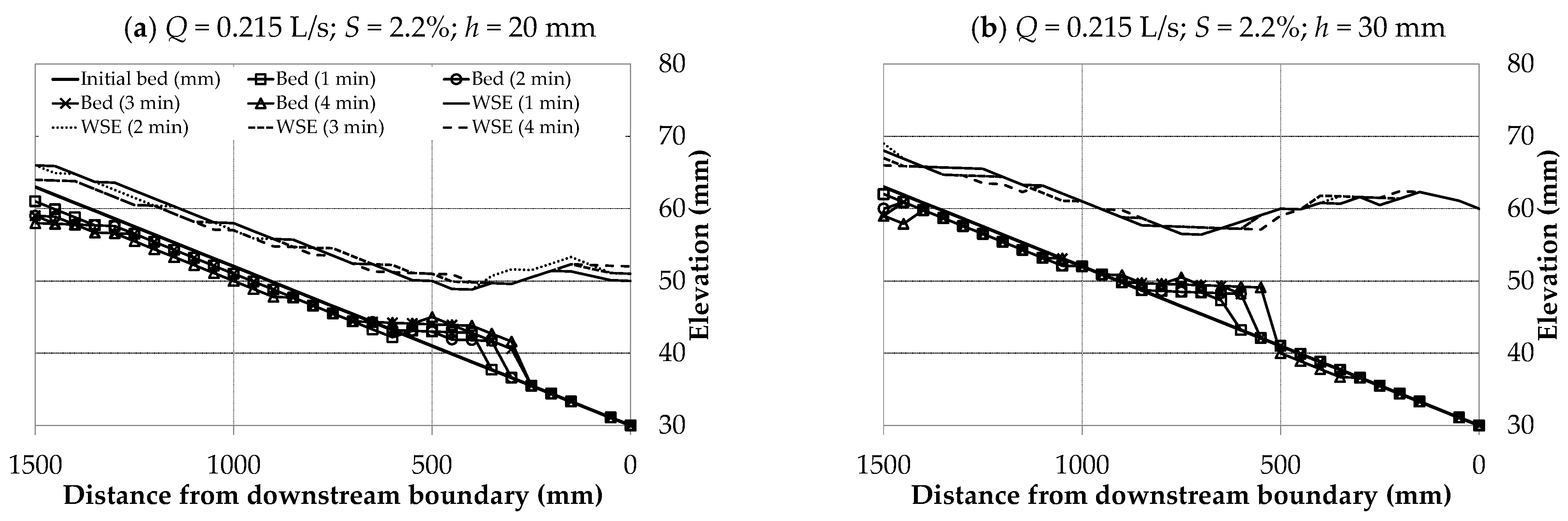
3.3. Numerical Results of STAFF Model

Due to limitations in experimental conditions, numerical simulations were performed for a total of 2646 conditions with respect to various discharges and sediment particle sizes in a range that could not be reproduced in laboratory experiments. Figure 4 shows the relationship between Ad and dimensionless variables.
As shown in Figure 4, Ad/qt showed a strong correlation in the order of dimensionless unit stream power, shields parameter, U*/ω, and D/ds. Consequently, in the laboratory experiment, it was decided to measure and analyze VS/ω, τ*, U*/ω, and D/ds.

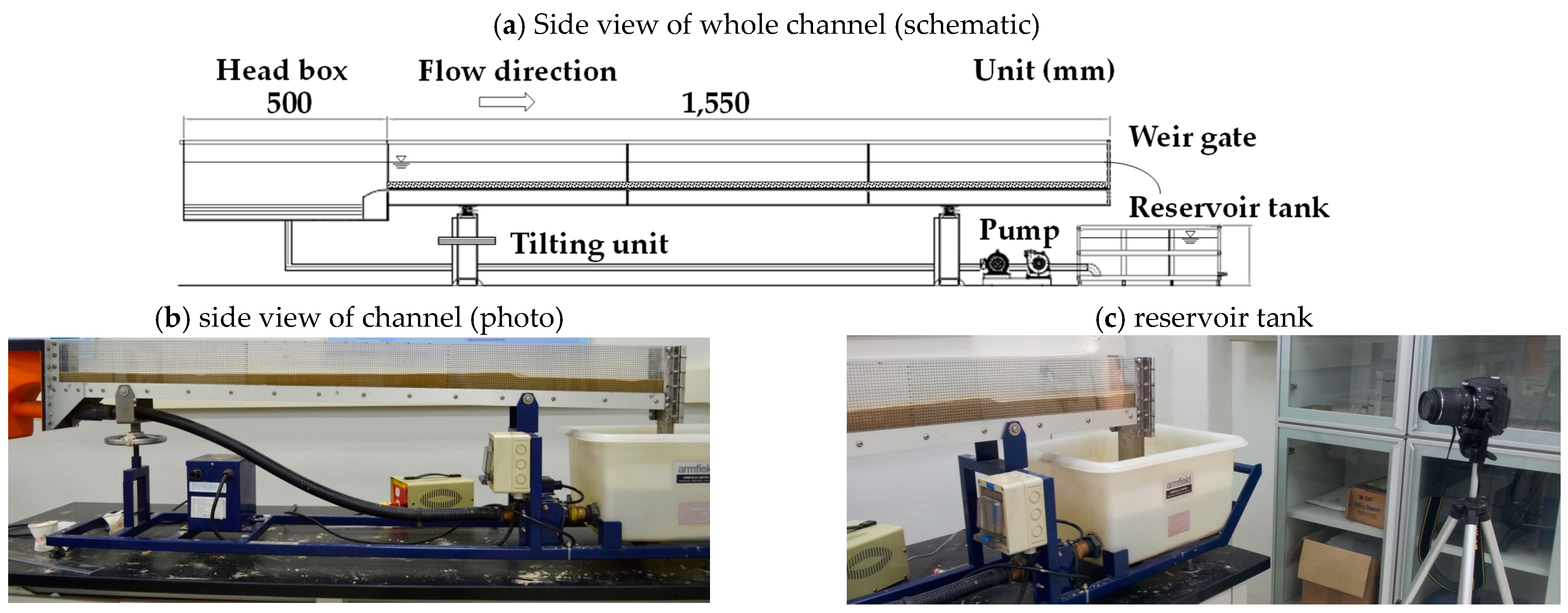
3.4. Experimental Setup and Measuring Apparatus

Sediment Channel-I (SC-I) which is a product (Product Code: S8-MKII) from Armfield ltd, is a flume of rectangular cross-section with dimensions of 78 mm in width, 1550 mm in length, and 110 mm in height. This flume offers the flexibility to apply various experimental conditions by adjusting the slope of the flume using a slope control device, allowing the bed slope to closely match that of natural rivers. At the downstream end of the flume, a multi-purpose weir model with adjustable height was manufactured and installed. It was modified to facilitate hydraulic model experiments in accordance with multi-purpose weir management water level operation (Figure 5).
The sediment channel-II (SC-II) is a flume with dimensions of 300 mm wide, 10,000 mm long, and 600 mm high. It was equipped with a slurry pump capable of circulating sediment particle. The inlet discharge range is from 0.6 to 8.0 L per second, and similar to SC-I, the flume’s slope can be finely adjusted in the vertical direction up to 500 mm. At the downstream part, a fixed weir model was installed to keep the water level consistent. Additionally, an upstream stabilizer with dimensions of 295 mm in width, 600 mm in length, and 100 mm in height was installed to prevent unexpectedly rapid erosion of the mobile bed by the flow originating from the head tank (Figure 6).

3.5. Experimental Procedure and Condition

In the SC-I experimental conditions, mobile bed experiments were conducted using three different sediment particles (with d50 = 0.20, 0.62, and 1.20 mm). Also, the previously mentioned ds was replaced by d50, which stands for median grain size (mm). A 5 mm scale was affixed to the right glass wall of the flume, covering a section of 1550 mm. Images were captured at 30-s intervals using a Digital Single Lens Reflex (DSLR) camera with 300 PPI (pixel per inch), allowing for the measurement of water surface and channel bed elevation at each time step under various experimental conditions through image processing and correlation analysis. Since the pixel size of the captured image is about 0.1 mm or less, which is less than the smallest d50 value of 0.2 mm, it was possible to prevent uncertainty that could occur in image processing.
In the case of the SC-II experiment, the adjustable slope system was designed to allow for slope adjustment within the range of 0% to 2.38%. At the downstream part, a fixed tailgate was installed to control the water depth. Sediment particle (d50 = 0.62 mm) was used, and for each experimental condition, the sediment was placed at a height of 100 mm from the floor, covering a 10,000 mm section of the test water. The experiment had a duration of 9 min, and measurements of bed elevation and water depth were taken five times: 1, 3, 5, 7, and 9 min later. Water depths were measured by wave height meter (CH-501, KENEK) with +/−0.5% linearity error and movable bed profiles were captured with using point gauge and water height sensor (WH-201C, KENEK) with +/−0.5 mm error range. The experiment commenced as soon as flow was introduced to the experimental waterway, precisely when backwater was initiated at the downstream end [35].

4. Results and Analysis

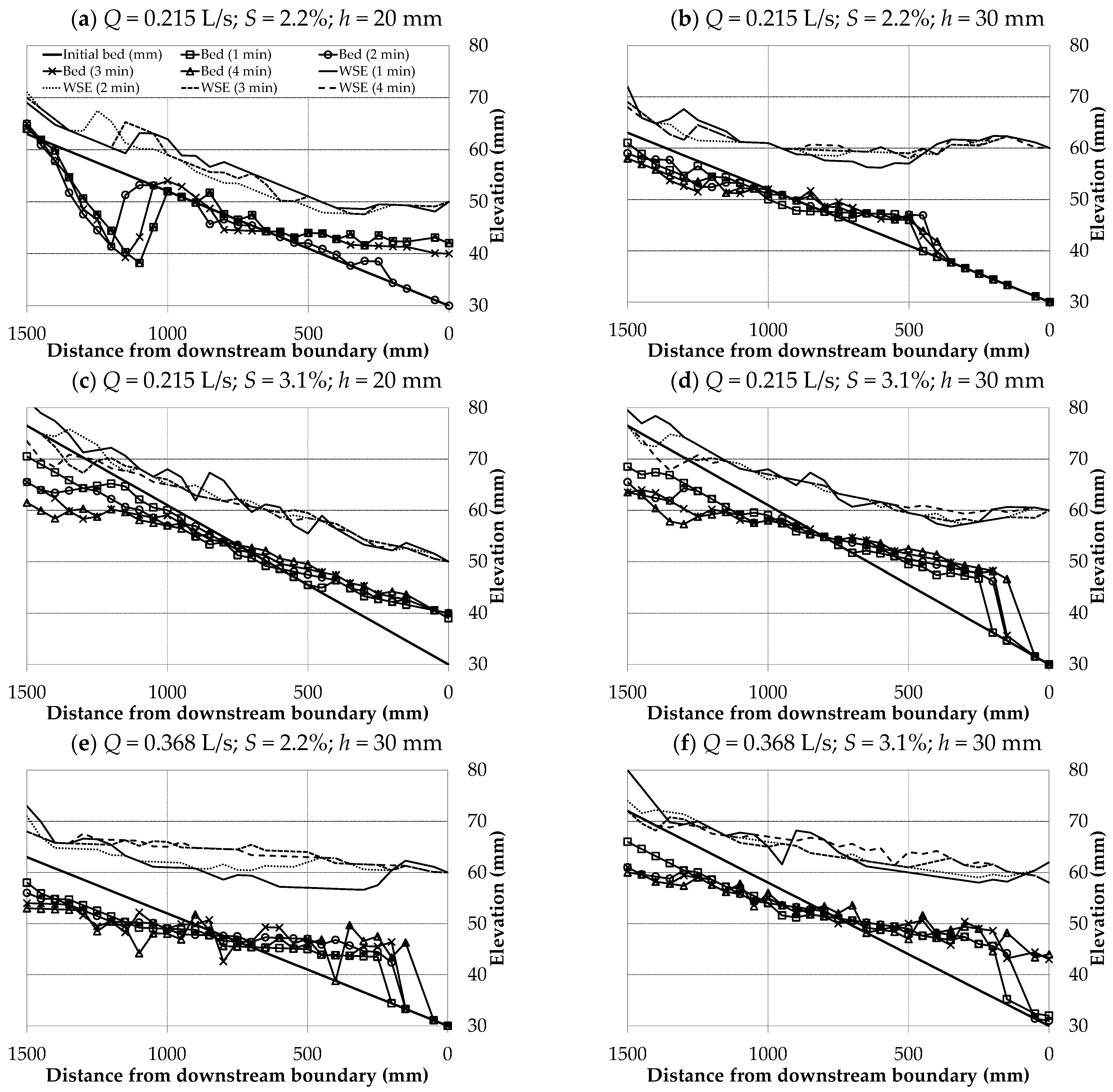
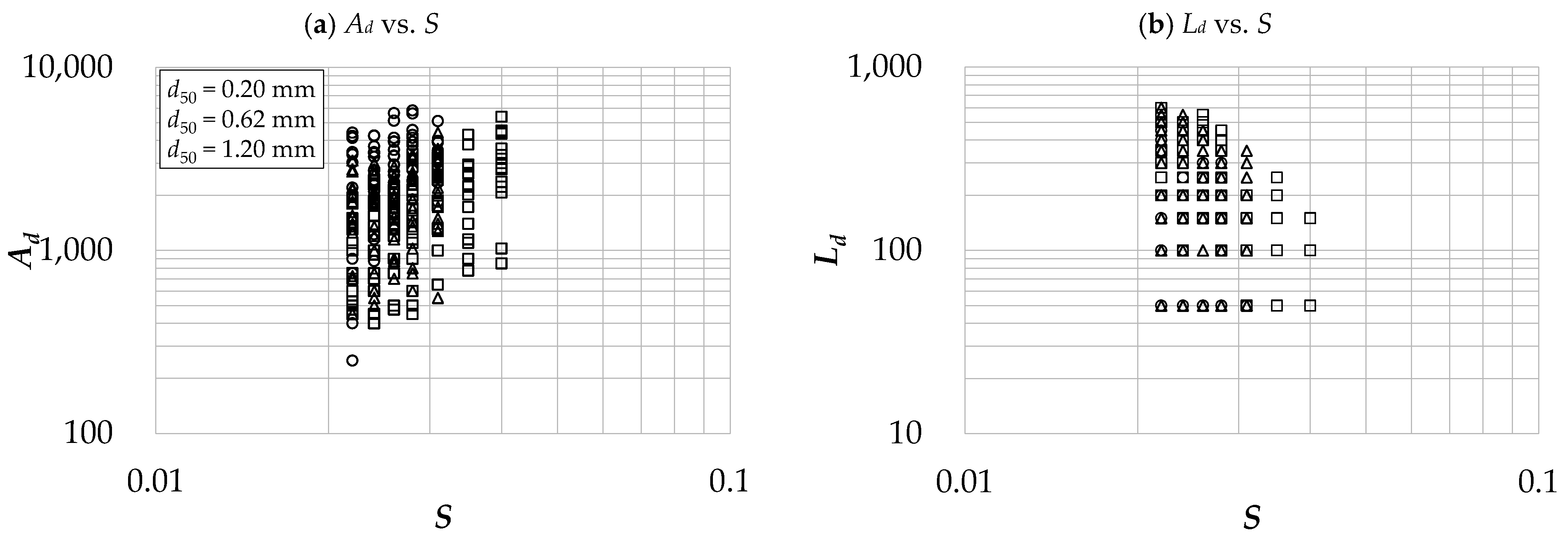
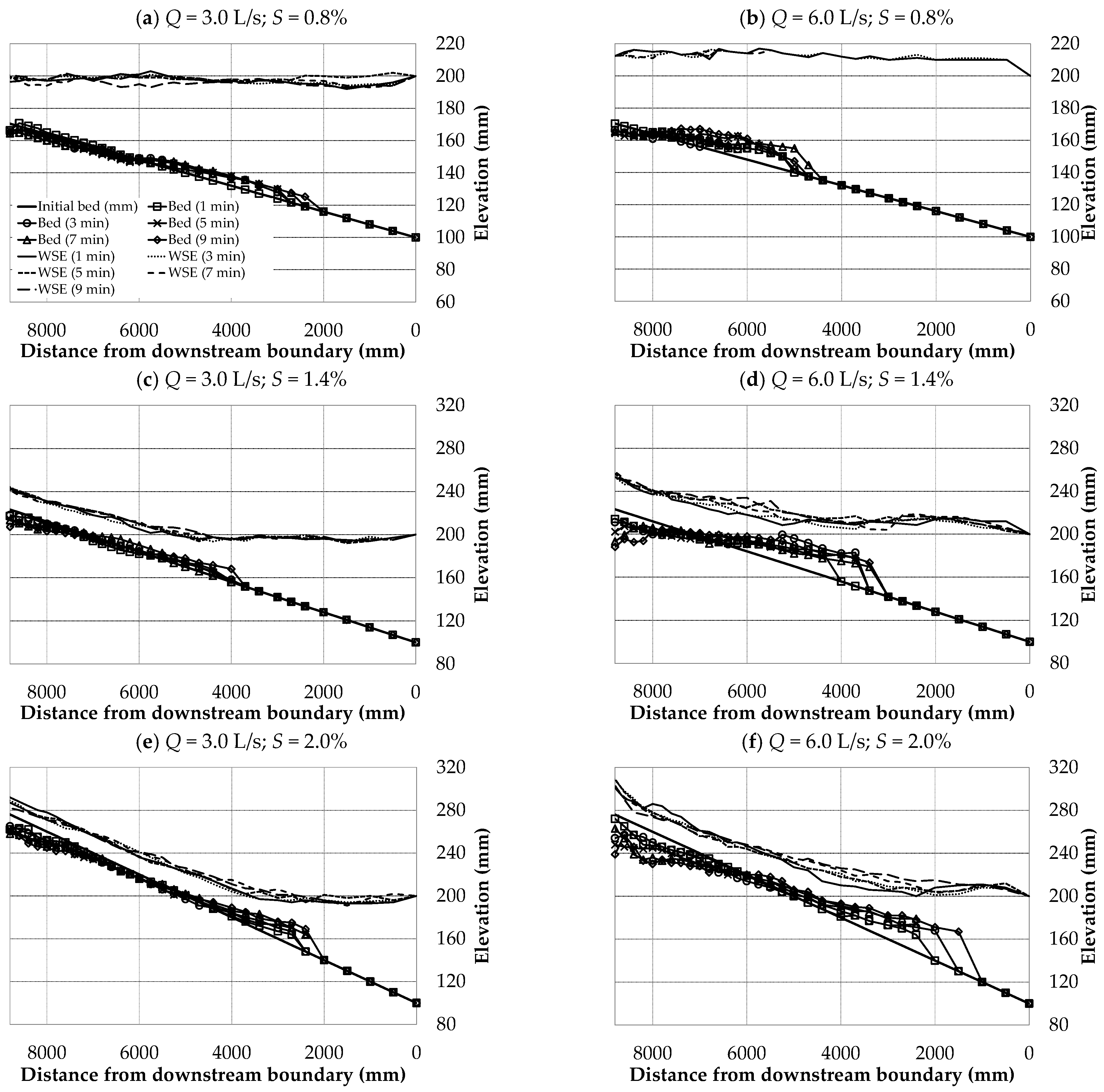
4.1. Experimental Results

Based on the experimental conditions presented in Table 1, changes in bed elevation and water depth over time are graphically shown (Figure 7). The initial bed profile is depicted with a bold line, and the upper lines without markers and the lower lines with markers represented the water surface elevation and bed elevation profiles for each time step, respectively. The experiment under the condition of d50 = 0.20 mm was conducted for 4 min each, and bed elevation and water depth were measured every minute to analyze variations of them over time. The scenario in which the water depth at the downstream end was 20 mm and the channel slope varied from 2.2% to 3.1% led to an expansion of the reservoir delta by approximately 50 mm in the stream-wise direction and an increase in bed elevation of about 4 mm in the depth-wise direction, as depicted in Figure 7a,c. Moreover, in the scenario where the water depth downstream was 30 mm and the channel slope also varied from 2.2% to 3.1%, it resulted in the expansion of the reservoir delta by approximately 250 mm in the stream-wise direction and 5 mm in the depth-wise direction (Figure 7b,d). Second, in a scenario where H = 30 mm and values of S changes to the same as the H = 20 mm condition, the reservoir delta grows by about 250 mm in the stream-wise direction and 5 mm in the depth-wise direction (Figure 7b,d). Through mass conservation calculations, it was confirmed that Ad increased by approximately 3.4 times, growing from 1500 mm2 to 5100 mm2 as the slope increased from 2.2% to 3.1%, as shown in Figure 7.
Temporal change of bed elevation profiles in the case with d50 = 0.62 mm were analyzed in a manner similar to that in the case with d50 = 0.20 mm. In other words, in the case of the minimum channel slope (=2.2%), the sediment deposition per unit width was calculated to be 3450 mm2, while for the maximum channel slope (=3.1%), Ad was estimated to be 7300 mm2, which is about 3.4 times larger (Figure 8).
For the case with d50 = 1.2 mm under the experimental conditions, Ad had a trend to increase by about 40% as the riverbed slope increased by 0.2%. Notably, lower downstream water depth resulted in a shorter period for the creation of the reservoir delta and a quicker decline in reservoir capacity (Figure 9). And, in the case of the d50 = 0.2 mm series under same experimental conditions, Ad increased by about 1.8 times as the flow discharge rose from 0.215 L/s to 0.368 L/s. However, for the series with similar particle size (d50 = 1.2 mm), Ad increased by approximately 2.6 times under the same experimental conditions, indicating that the series with a larger sediment particle was more sensitive to changes in flow rate compared to the series with a smaller sediment particle (Figure 9). The overall relationship between Ad and Ld versus S were plotted and compared in Figure 10.
Changes in bed elevation and water depth by time step and experimental condition of the SC-II experiment are shown in Figure 10. In the case of Ad, it was proportional to flow rate and riverbed slope, similar to the SC-I experiment results. In addition, when the flow rate is fixed at 6 L/s, the sedimentation amount at 1 min after the start of the experiment is 3.27 times that of 9 min when the riverbed slope is 1.4%, but 4.53 times at 2.0%. With an increase of 0.6%, the sediment amount increased by about 140%. Comparing the bed slope and water depth graphs in Figure 9c,d of the experimental results with bed slope of 1.4% and 2.0%, in the experimental condition of 1.4%, the backwater region is about 4.2 m away from the downstream weir body. However, at 2.0%, the backwater region is generated with a length of 2.4 m, making the backwater region shorter by about 40%. Ld, the distance from the downstream weir body to the reservoir start point, tended to decrease by 50% as the slope of flume increased from 1.4% to 2.0%.
In Figure 11, we plotted the water depth and channel bed elevation of SC-II cases.

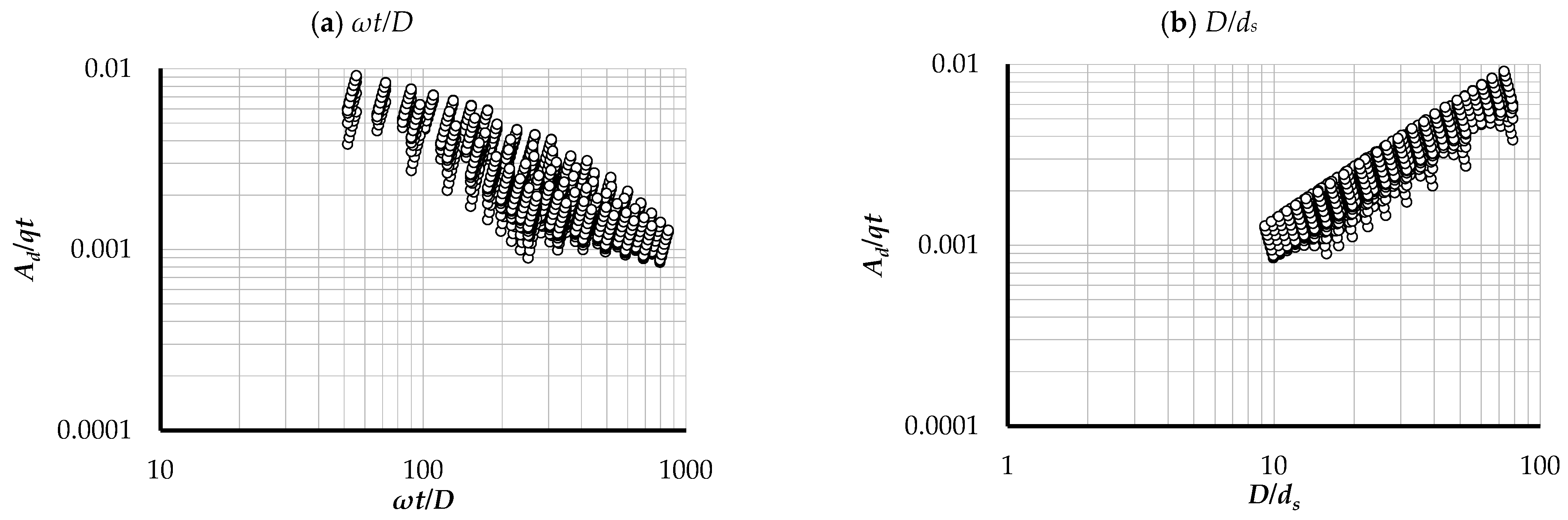
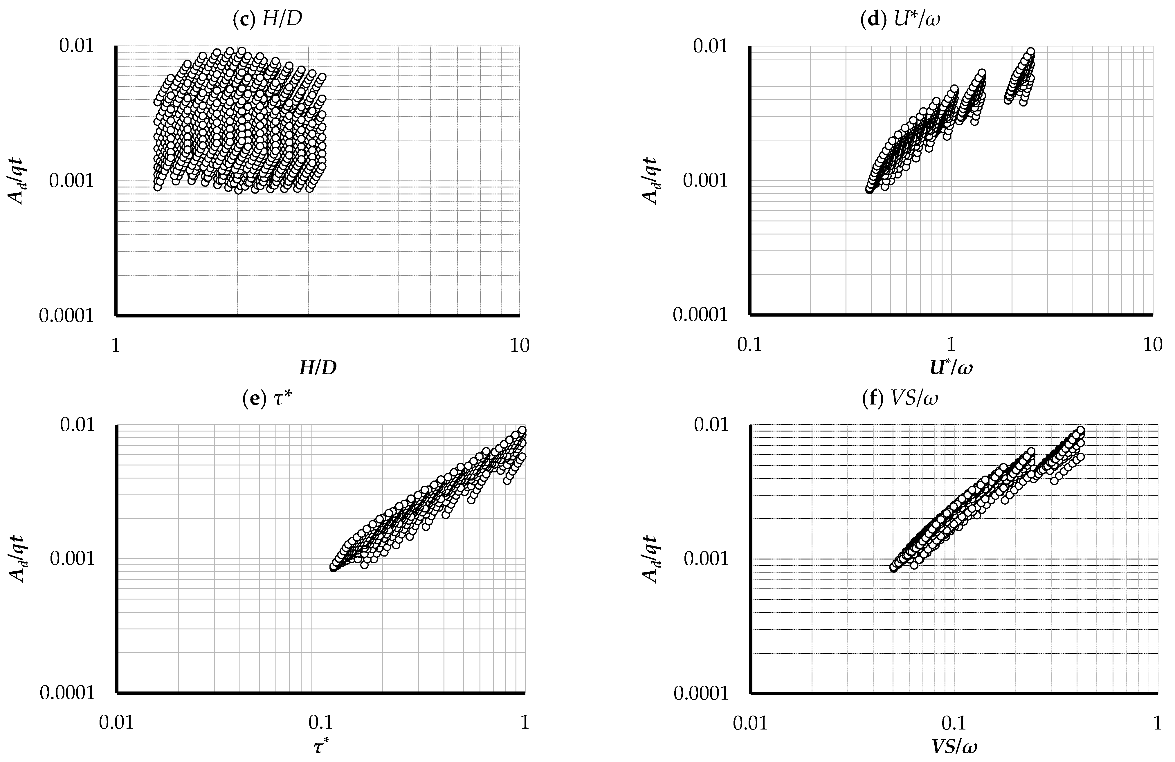
4.2. Derivation of Empirical Equation
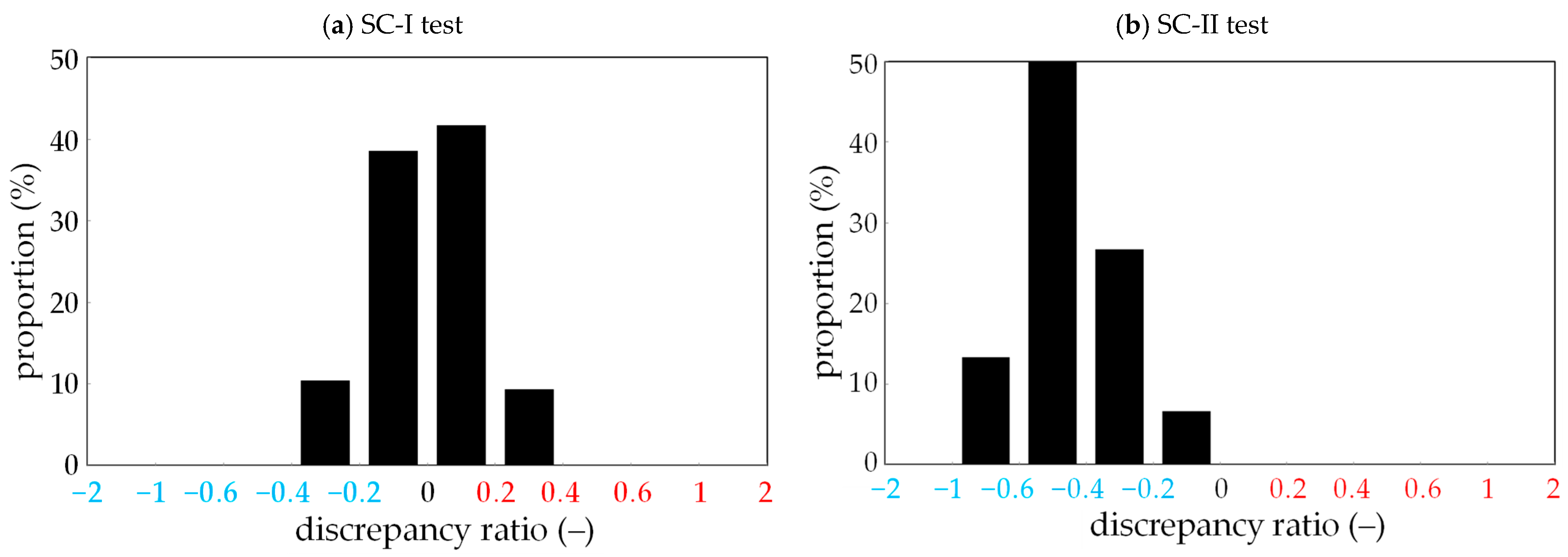
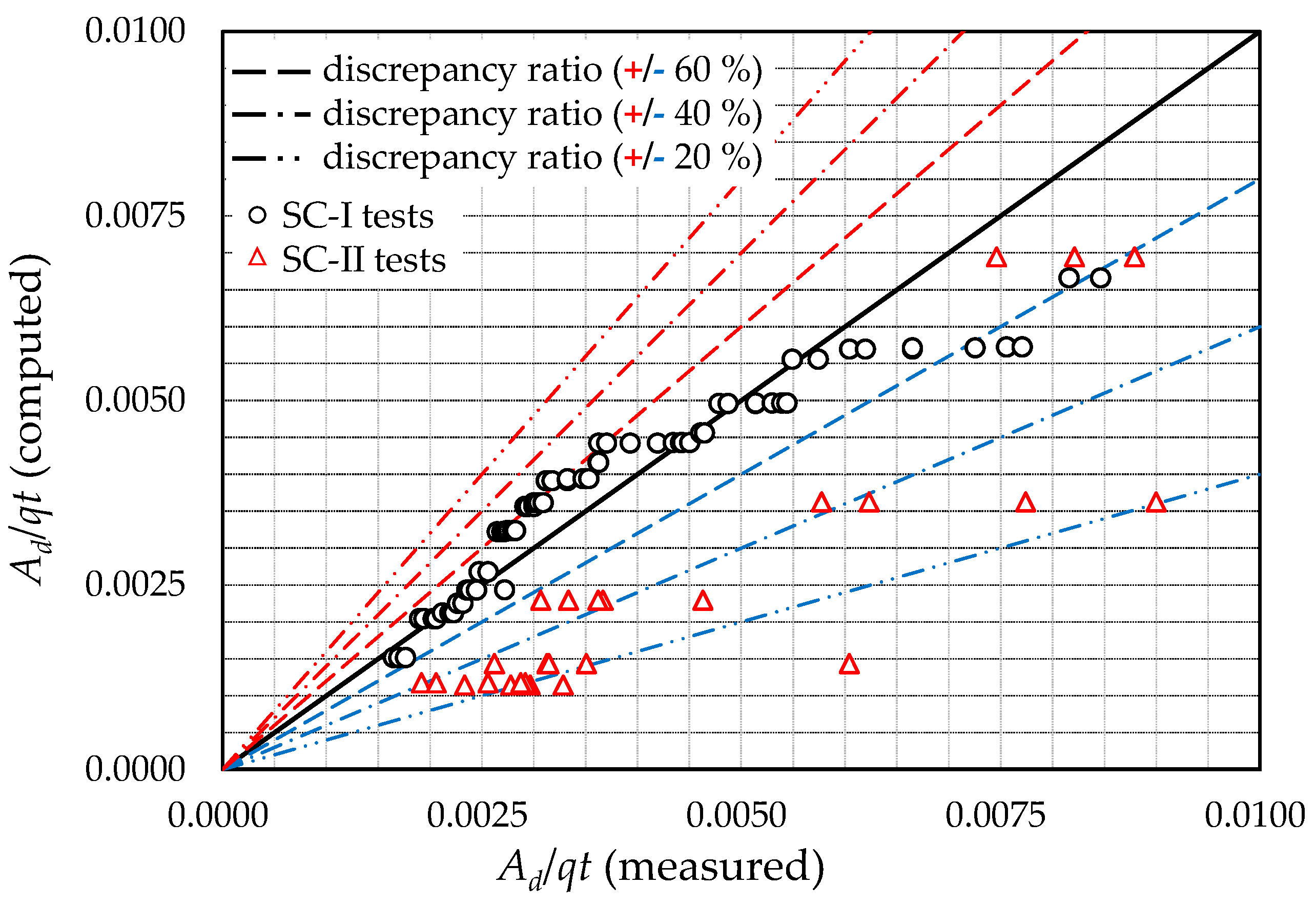
The correlation analysis between Ad/qt and dimensionless parameters is shown in Figure 12 with the regression curves. To identify the parameters with the highest correlation to Ad/qt, statistical analysis was conducted in Table 2. As a result, dimensionless unit stream power, Shields parameter, U*/ω, and D/d50 were analyzed to have the highest correlation. In this study, a nonlinear multiple regression method was applied to develop an empirical equation that can be used to predict the sedimentation behavior of upstream reservoirs. The 288 experimental result data calculated through SC-I cases were randomly classified into 192 and 96 terms for derivation and verification of the empirical equation. In addition, in order to understand the statistical characteristics of the two data sets, the range, median, and quartile values of VS/ω, Ad/qt, and τ* for each term were analyzed and presented in Table 3.
The empirical equation as a result of deriving the multiple regression analysis equation using 192 experimental result datasets among the SC-I experiment data is as follows:
A d q t = 0.024 V S ω 1.111 τ * 0.049
In the derivation of this equation, the correlation coefficient was analyzed to be 0.91 and the standard deviation was 0.00071.

4.3. Error Analysis

The empirical equation derived in this study was verified using 96 datasets out of 288 SC-I experiment results and 30 datasets acquired from SC-II experiment. Figure 13 showed the discrepancy ratio, where the correlation can be seen through a 1:1 graph between the computed results calculated using Equation (23) and the measured data.
Figure 14 shows the discrepancy rates for the SC-I experiment and SC-II experiment, respectively.
Error analysis with the RMSE (Root Mean Square Error), MAE (Mean Absolute Error), and AGD (Averaged Geometric Deviation) were calculated with 96 and 30 datasets of SC-I and SC-II test, respectively (Table 4). The SC-I data showed a smaller error than the SC-II data, and it was found that the SC-II experimental conditions were under-predicted with the empirical equation.
RMSE = j = 1 J Z c j Z m j 2 / J 1 / 2
MAE = 1 J j = 1 J Z c j Z m j
AGD = j = 1 J R j 1 / J , R j Z c j / Z m j Z m j / Z c j for   Z c j Z m j Z m j Z c j
Herein, Zc represents the dimensionless sediment deposition calculated using the empirical equation, while Zm represents the dimensionless sediment deposition measured through experiments. J denotes the number of experiments and Rj represents the special discrepancy ratio. The verification results are presented in Table 4 and are derived from the analysis of the Pearson correlation coefficient. Accordingly, it was determined that there was a strong positive correlation.

5. Summary of Research

In this study, numerical analysis and mobile bed experiments were performed to investigate the behavior of the reservoir delta deposited upstream of a weir model in rivers and streams. Using the one-dimensional uncoupled numerical approach for the calculation of flow and sediment transport, six dominant factors of the laboratory experiment including dimensionless unit stream power, Shields parameter, ratio of shear velocity and fall velocity, ratio of upstream normal depth, and sediment particle size were determined.
From the experimental approach, it was observed that the formation and evolution of a reservoir delta are significantly influenced by four key factors: sediment particle size, channel slope, flow discharge, and downstream water depth. In particular, as the channel slope increased by 0.1%, the sediment deposition increased by approximately 12%. This was confirmed through both experimental results and predictions based on empirical equations. Under the experimental conditions with a channel slope of 0.8%, there was no backwater observed. The 10 meter long test section was affected by the downstream boundary. In other words, all reach is under backwater condition. However, at a channel slope of 1.4%, backwater was generated, extending approximately 4.2 m. As the channel slope increased to 2.0%, the length of backwater tended to decrease by about 2.6 m. Nevertheless, when the water depth, which maintained a slope nearly parallel to the channel bed, encountered the backwater section, the slope abruptly decreased to nearly 0%, resulting in a rapid reduction of flow and subsequent sedimentation as previously revealed [36].
As a result of one-dimensional numerical simulation, reservoir delta was found to be significantly influenced by four conditions: diameter of sediment particle, bed slope, inlet discharge, and water depth at downstream. Correlation analysis of dimensionless sediment deposition per unit width (Ad/qt) and dimensionless hydraulic and sediment parameters (time, flow rate, fall velocity of sediment particle, unit stream power, water depth at the weir gate, friction velocity, bed slope) Through this, multiple regression equations consisting of dimensionless unit stream power and Shields parameter, which have the greatest correlation, were derived. As a result of statistical analysis through application of the derived empirical formula, RMSE was 0.0007, MAE was 0.0005, and AGD was 1.0390, indicating that the range was quite acceptable.
In particular, sedimentation patterns were observed to differ according to the experimental conditions when there was significant variation in water depth. Therefore, additional research is deemed necessary to address issues related to reservoir capacity and potential degradation of flood stages.

6. Conclusions and Future Direction

The conventional previous studies indicated that the reservoir sedimentation rate is affected by the basin sediment yield and delivery ratio. However, this study focused on current channel condition, without considering basin sediment yield, to predict the rate of reservoir sedimentation by assuming the upstream cross section of reservoir region was in equilibrium state. Because the amount of basin sediment yield and the delivery ratio are very difficult to predict, this study assumed that the present channel water and sediment discharges, before construction of weir, were already formed by the basin sediment loss and delivery ratio. On the other hand, it was found that bed elevation changes, which vary with flow, including shear velocity, Shields parameter, and unit stream power based on channel slope and flow discharge in natural rivers, are suitable for the development of reservoir deltas. As a result of predicting the sedimentation amount in experiments using the developed empirical formula, there was a tendency for the predicted sedimentation amount to be somewhat lower than that observed in the smaller scaled experiments (SC-I experiment). This phenomenon can be improved through further research that considers changes in inlet discharge, sediment particle size, and downstream water depth using medium- to large-scale experimental channels.
There are two primary limitations in this study. Firstly, to simulate and analyze the development of the reservoir delta and backwater effect upstream of a weir or dam more closely to real-world conditions, it is essential to account for or replicate sediment particle influx from upstream. This aspect can be explored as a future research direction. Secondly, a comprehensive analysis of width-wise variations is required. While the mechanisms in the stream-wise direction play a dominant role in sediment transport and flow regime, ensuring field applicability in the future can be achieved by examining the behavior characteristics with additional consideration for width-wise variations, accounting for weighted or attenuated effects. Overcoming the aforementioned limitations, the empirical formula established in this study can be employed in two future directions with dominant dimensionless parameters. Firstly, it can be referred for low-head dams or multi-purpose weir fate planned for construction in upcoming reservoir projects to predict short- and long-term sedimentation volumes in advance. This information can be utilized to plan for reservoir capacity and sedimentation management. Additionally, it can provide valuable insights into the limitations, dimensions, and requirements for related additional structures when constructing riverine hydraulic facilities. Notably, the empirical formula’s application can substitute the need for time-consuming and labor-intensive long-term researches or field measurements when determining deposition in the reservoir delta, suggesting the possibility of using it for the delta deposition management and flushing. Secondly, the hydraulic similitude applied in this study can contribute to establishing experimental conditions for hydraulic experimental modeling. This will be beneficial for studying long-term deposition and flushing operation management methods in the future. Unlike fixed bed modeling, it is expected that similitude can be more easily achieved by using the method described in this paper for mobile bed modeling, where applying similitude is typically challenging.

Author Contributions

J.A. was responsible for conceptualization, methodology and software application of this research. J.A. and S.W.P. were involved in model validation, data curation and writing—original draft preparation. S.W.P. and C.G.S. were involved in writing—review and editing. C.G.S. contributed to supervision, project administration and funding acquisition. All authors have read and agreed to the published version of the manuscript.

Funding

This study was supported by Korea Environment Industry & Technology Institute (KEITI) through Environmental R&D Project on the Disaster Prevention of Environmental Facilities, funded by Korea Ministry of Environment (MOE) (2022002850001).

Data Availability Statement

The data presented in this study area available on request from the corresponding author.

Conflicts of Interest

The authors declare no conflict of interest.

Nomenclature

SymbolsDefinitions
AdSediment load amount per unit width
LdStream-wise distance from the main body of the multi-purpose weir to the starting point of the reservoir delta in Figure 1
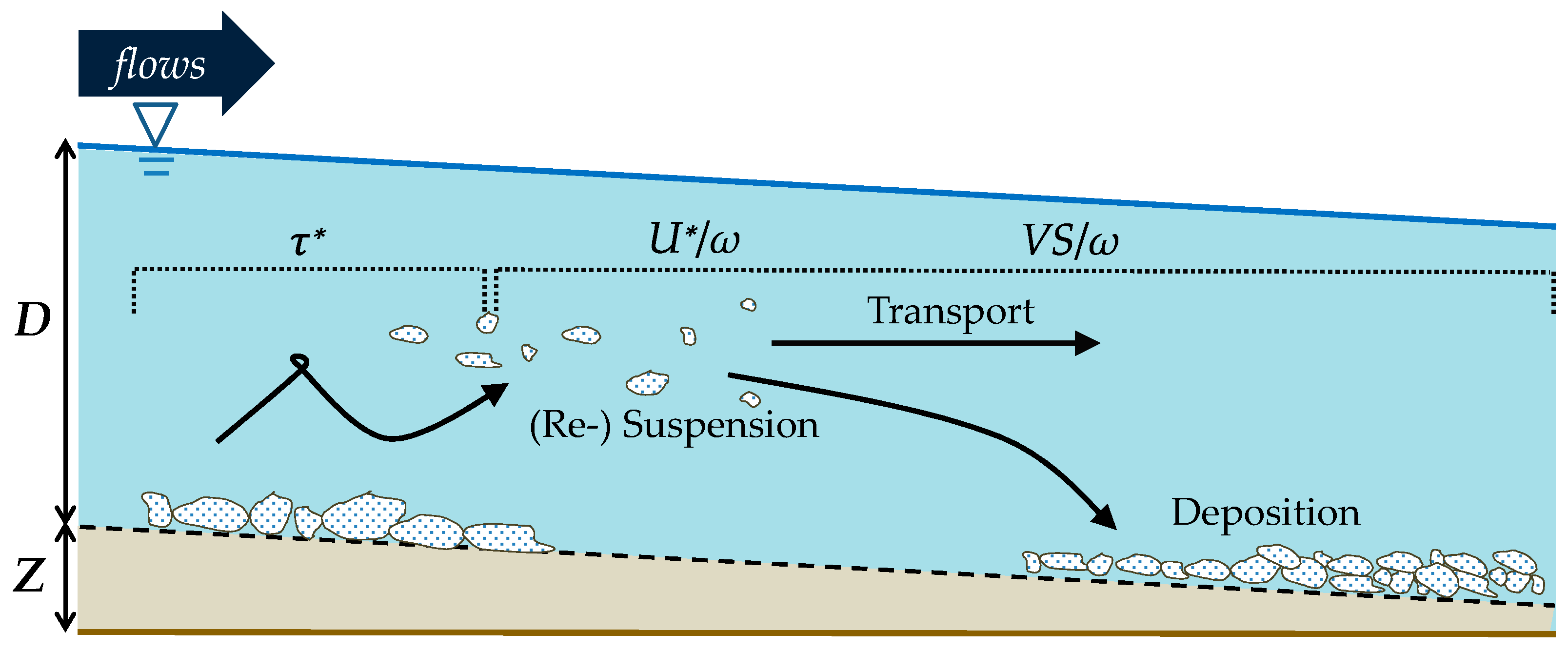
VSUnit stream power in Figure 2
V and SFlow velocty and river bed slope in Figure 2
VS/ωNon-dimensional unit stream power in Figure 2
ωFall velocity in Figure 2
U*Friction velocity in Equation (1)
U*/ωRatio of the friction veocity in Equation (1)
RHydraulic radius in Equation (1)
gGravitational acceleration
τ*Shields paramete in Equation (2)
τ0Bed shear stress in Equation (2)
γSpecific weight of water in Equation (2)
GSpecific gravity of sediment, Equation (2)
dsSediment particle size in Equation (2)
hWater surface elevation in Equation (3)
βEnergy coefficient in Equation (3)
hLEnergy loss in Equation (3)
SfFriction slope in Equation (4)
ΔxStream-wise distance in Equation (4)
qdischarge per unit width in Equations (6) and (7)
ZBed elevation from datum in Figure 1 and Figure 2, Equations (7) and (9)
nManning’s roughness coefficient in Equations (8) and (9)
CwSediment concentration by weight in Equations (11) and (12)
CvSediment concentration by volume in Equation (12)
qsSediment discharge per unit width in Equation (13)
pPorosity of soil in Equation (14)
tTime in Equation (14)
xStream-wise length in Equation (15)
ΔZBed elevation change in Equation (15)
ΔtTime step in Equation (15)
j and kSpatial and temporal index in Equation (15)
ρDensity of fluid in Equation (16)
νKinematic viscosity in Equation (16)
DUpstream normal depth in Equation (16)
CuSediment non-uniformity constant in Equation (16)
CtSediment concentration in parts per million by weight in Equation (22)
Vccritical average flow velocity in incipient motion in Equation (22)
ZcDimensionless sediment deposition caculated using equation
ZmDimensionless sediment deposition measured by experiments
JNumber of experiments
RjSpecial discrepancy ratio

References

  1. Morris, G.L.; Fan, J. Reservoir Sedimentation Handbook: Design and Management of Dams, Reservoirs, and Watersheds for Sustainable Use; McGraw-Hill: New York, NY, USA, 1998. [Google Scholar]
  2. Anton, J.S.; Mário, J.F.; Carmelo, J.; Giovanni, D.C. Reservoir sedimentation. J. Hydraul. Res. 2016, 54, 595–614. [Google Scholar] [CrossRef]
  3. Julien, P.Y. Erosion and Sedimentation; Cambridge University Press: New York, NY, USA, 1995. [Google Scholar] [CrossRef]
  4. White, R. Evacuation of Sediments from Reservoirs; Thomas Telford Publishing: London, UK, 2001. [Google Scholar] [CrossRef]
  5. Toniolo, H.; Parker, G. 1D numerical modeling of reservoir sedimentation. In Proceedings of the IAHR Symposium on River, Coastal and Estuarine Morphodynamics, Barcelona, Spain, 1–5 September 2003. [Google Scholar]
  6. Wright, L.D.; Coleman, J.M. Mississippi river mouth processes: Effluent dynamics and morphologic development. J. Geol. 1974, 82, 751–778. [Google Scholar] [CrossRef]
  7. Soni, J.P.; Ranga Raju, K.G.; Garde, R.J. Aggradation in streams due to overloading. J. Hydraul. Div. 1980, 106, 117–132. [Google Scholar] [CrossRef]
  8. Hotchkiss, R.H. Reservoir Sedimentation and Sluicing: Experimental and Numerical Analysis; St. Anthony Falls Hydraulic Laboratory: Minneapolis, MN, USA, 1990; Available online: https://hdl.handle.net/11299/108511 (accessed on 12 November 2023).
  9. Hotchkiss, R.H.; Parker, G. Shock fitting of aggradational profiles due to backwater. J. Hydraul. Eng. 1991, 117, 1129–1144. [Google Scholar] [CrossRef]
  10. Yang, C.T.; Simões, F.J.M. GSTARS Computer Models and Their Application, part I: Theoretical Development. Int. J. Sediment Res. 2008, 23, 197–211. [Google Scholar] [CrossRef]
  11. Simões, F.J.M.; Yang, C.T. GSTARS Computer Models and Their Applications, Part II: Applications. Int. J. Sediment Res. 2008, 23, 299–315. [Google Scholar] [CrossRef]
  12. Yang, C.T. Discussion of “Sediment Transport Modeling Review—Current and Future Developments” by A.N. Papanicolaou, M. Elhakeem, G. Krallis, S. Prakash, and J. Edinger. J. Hydraul. Eng. 2010, 136, 552–555. [Google Scholar] [CrossRef]
  13. Fan, J.; Morris, G.L. Reservoir sedimentation I: Delta and density current deposits. J. Hydraul. Eng. 1992, 118, 354–369. [Google Scholar] [CrossRef]
  14. Fan, J.; Morris, G.L. Reservoir sedimentation II: Reservoir desiltation and long-term storage capacity. J. Hydraul. Eng. 1992, 118, 370–384. [Google Scholar] [CrossRef]
  15. Ahn, J.; Yang, C.T.; Boyd, P.M.; Pridal, D.B.; Remus, J.I. Numerical modeling of sediment flushing, from Lewis and Clark Lake. Int. J. Sediment Res. 2013, 28, 182–193. [Google Scholar] [CrossRef]
  16. Choi, H. Experimental Investigation of Sedimentation at Multi-Purposed Weir. Master’s Thesis, Seoul National University, Seoul, Republic of Korea, 2014. Available online: https://s-space.snu.ac.kr/handle/10371/124243 (accessed on 12 November 2023). (In Korean).
  17. Kantoush, S.A.; Bollaert, E.; Schleiss, A.S. Experimental and numerical modelling of sedimentation in a rectangular shallow basin. Int. J. Sediment Res. 2008, 23, 212–232. [Google Scholar] [CrossRef]
  18. Gökçen, B.; Güney, M.S. Experimental investigation of sediment transport in steady flows. Sci. Res. Essays 2008, 5, 582–591. [Google Scholar]
  19. Dufresne, M.; Dewals, B.; Erpicum, S.; Archambeau, P.; Pirotton, M. Flow patterns and sediment deposition in rectangular shallow reservoirs. Water Environ. J. 2012, 26, 504–510. [Google Scholar] [CrossRef]
  20. Souza, L.B.S.; Schulz, H.E.; Villela, S.M.; Gulliver, J.S. Experimental study and numerical simulation of sediment transport in a shallow reservoir. J. Appl. Fluid Mech. 2010, 3, 9–21. [Google Scholar] [CrossRef]
  21. Bui, V.H.; Bui, M.D.; Rutschmann, P. Advanced Numerical Modeling of Sediment Transport in Gravel-Bed Rivers. Water 2019, 11, 550. [Google Scholar] [CrossRef]
  22. Latif, S.D.; Chong, K.L.; Ahmed, A.N.; Huang, Y.F.; Sherif, M.; El-Shafie, A. Sediment load prediction in Johor River: Deep learning versus machine learning models. Appl. Water Sci. 2023, 13, 79. [Google Scholar] [CrossRef]
  23. Legowo, S.; Hadihardaja, I.K.; Azmeri, A. Estimation of Bank Erosion Due to Reservoir Operation in Cascade (Case Study: Citarum Cascade Reservoir). J. Eng. Technol. Sci. 2013, 41, 148–166. [Google Scholar] [CrossRef]
  24. Yang, C.T. Unit stream power equations for total load. J. Hydrol. 1979, 40, 123–138. [Google Scholar] [CrossRef]
  25. Shields, A. Application of Similarity Principles and Turbulence Research to Bed-Load Movement; California Institute of Technology: Pasadena, CA, USA, 1936; (Translated from German). [Google Scholar]
  26. Brunner, G.W. HEC-RAS River Analysis System: Hydraulic Reference Manual, Version 5.0; US Army Corps of Engineers–Hydrologic Engineering Center, 547: Davis, CA, USA, 2016. Available online: https://www.hec.usace.army.mil/software/hec-ras/documentation/ (accessed on 2 December 2023).
  27. Lai, Y.G.; Gaeuman, D. SRH-2D User’s Manual: Sediment Transport and Mobile-Bed Modeling; US Bureau of Reclamation: Washington, DC, USA, 2009; Volume 179.
  28. Deltares. Delft3D-Flow. Simulation of Multi-Dimensional Hydrodynamic Flows and Transport Phenomena, Including Sediments: User manual; Deltares: Delft, The Netherlands, 2010. [Google Scholar]
  29. Engelund, F.; Hansen, E. A Monograph on Sediment Transport in Alluvial Streams; Tekniskforlag: Copenhagen, Denmark, 1967; Available online: http://resolver.tudelft.nl/uuid:81101b08-04b5-4082-9121-861949c336c9 (accessed on 2 December 2023).
  30. Lee, J.M.; Ahn, J. Analysis of Bed Sorting Methods for One Dimensional Sediment Transport Model. Sustainability 2023, 15, 2269. [Google Scholar] [CrossRef]
  31. Kim, S.K.; Kim, J.S.; Kim, K.H.; Choi, S.U. Prediction and Historical Analysis of Long-Term Bed Elevation Change in the Mankyung-Gang River. Ecol. Resilient Infrastruct. 2018, 5, 25–34. (In Korean) [Google Scholar] [CrossRef]
  32. Exner, F.M. Über die wechselwirkung zwischen wasser und geschiebe in flüssen. Sitzungsberichte Akad. Wiss. Math. Naturwissenschaftliche Kl. 1925, 134, 165–203. [Google Scholar]
  33. Dodaro, G.; Tafarojnoruz, A.; Sciortino, G.; Adduce, C.; Calomino, F.; Gaudio, R. Modified Einstein Sediment Transport Method to Simulate the Local Scour Evolution Downstream of a Rigid Bed. J. Hydraul. Eng. 2016, 142, 04016041. [Google Scholar] [CrossRef]
  34. Yang, C.T. Incipient Motion and Sediment Transport. J. Hydraul. Div. 1973, 99, 1679–1704. [Google Scholar] [CrossRef]
  35. Park, S.W.; Hwang, J.H.; Ahn, J. Physical Modeling of Spatial and Temporal Development of Local Scour at the Downstream of Bed Protection for Low Froude Number. Water 2019, 11, 1041. [Google Scholar] [CrossRef]
  36. Wang, L.; Cuthbertson, A.; Pender, G.; Zhong, D. Bed load sediment transport and morphological evolution in a degrading uniform sediment channel under unsteady flow hydrographs. Water Resour. Res. 2019, 55, 5431–5452. [Google Scholar] [CrossRef]
Figure 1. Schematic diagram of reservoir delta deposition at the upstream of weir gate.
Water 16 00574 g001
Figure 2. Schematic diagram of reservoir sedimentation and dimensionless.
Water 16 00574 g002
Figure 3. Flow chart of STAFF model calculation.
Water 16 00574 g003
Figure 4. Results of STAFF model (2646 cases).
Water 16 00574 g004aWater 16 00574 g004b
Figure 5. Experimental sediment channel-I (SC-I) and its arrangement (revised from Choi [16]).
Water 16 00574 g005
Figure 6. Experimental channel (SC-II) and setup (revised from Choi [16]): (a) side view of whole channel; (b) headbox with flow stabilizer and honey comb walls; (c) measuring apparatus with the auto-traverse; (d) tailgate at the channel end and reservoir tank.
Water 16 00574 g006
Figure 7. Comparison of delta deposition of SC-I experiments with d50 = 0.20 mm.
Water 16 00574 g007
Figure 8. Comparison of delta deposition of SC-I experiments with d50 = 0.62 mm.
Water 16 00574 g008
Figure 9. Comparison of delta deposition of SC-I experiments with d50 = 1.20 mm.
Water 16 00574 g009aWater 16 00574 g009b
Figure 10. Relationship between deposition ridge properties (volume and length) and channel slope.
Water 16 00574 g010
Figure 11. Delta deposition of SC-II experiments (d50 = 0.62 mm; h = 100 mm).
Water 16 00574 g011
Figure 12. Relationship between Ad/qt and dimensionless hydraulic parameters.
Water 16 00574 g012
Figure 13. Comparison between measured and computed results.
Water 16 00574 g013
Figure 14. Discrepancy ratios for two data sets.
Water 16 00574 g014
Table 1. Experimental conditions and parameters’ ranges.
Types No. of CasesS
(%)
Q
(L/s)
H
(mm)
Re
(= 4 V R / ν )
Fr
(= V / g H )
d50
(mm)
D/d50
(−)
U*/ω
(−)
τ*
(Pa)
VS/ω
(−)
SC-I
tests
2882.2
−4.0
0.215
−0.368
20
−30
1049
−1773
0.061
−0.057
0.20
−1.20
2.5
−75.0
0.315
−2.46
0.0606
−1.188
0.0796
−0.650
SC-II
tests
300.8
−2.0
3–61009231
−18,462
0.050
−0.101
0.6225.8
−45.2
0.488
−0.905
0.1251
−0.430
0.0021
−0.0188
Table 2. Comparison of R2 between numerical modeling and experimental research for parameters.
ParameterD/dsU*/ωτ*/ωVS/ω
Numerical Simulation0.88540.90420.90520.9451
SC-I Experiments0.10810.20020.21100.3743
Table 3. Statistical characteristics of data sets (SC-I Experiments).
ParameterDerivation Data SetVerification Data Set
RangeMeanQuartileRangeMeanQuartile
Ad/qt0.0015–0.01420.00390.00250.0027–0.00850.00360.0028
VS/ω0.0796–0.40240.22000.13070.1392–0.33560.21760.1720
τ*0.6000–1.18790.12250.08880.1290–0.23460.16810.1350
Table 4. Statistical analysis for verification results.
Experimental CaseData SetRMSEMAEAGD
SC-I test960.00070.00051.0390
SC-II test300.00390.00261.1161
Disclaimer/Publisher’s Note: The statements, opinions and data contained in all publications are solely those of the individual author(s) and contributor(s) and not of MDPI and/or the editor(s). MDPI and/or the editor(s) disclaim responsibility for any injury to people or property resulting from any ideas, methods, instructions or products referred to in the content.

