Study on Numerical Simulation of Reactive-Transport of Groundwater Pollutants Caused by Acid Leaching of Uranium: A Case Study in Bayan-Uul Area, Northern China

Abstract

Acid in situ leaching (ISL) is a common approach to the recovery of uranium in the subsurface. In acid ISL, there are numerous of chemical reactions among the injected sulfuric acid, groundwater, and porous media containing ore layers. A substantial amount of radioactive elements including U, Ra, Rn, as well as conventional elements like K, Na, and Ca, and trace elements such as As, Cd, and Pb, are released into the groundwater. Thus, in acid ISL, understanding the transport and reactions of these substances and managing pollution control is crucial. In this study, a three-dimensional reactive transport modeling (RTM) using TOUGHREACT was built to investigate the dynamic reactive migration process of UO₂²⁺, H⁺, and SO₄²⁻ at a typical uranium mine of Bayan-Uul. The model considering the partial penetration through wellbore in confined aquifer and complex chemical reactions among main minerals like uranium, K-feldspar, calcite, dolomite, anhydrite, gypsum, iron minerals, clay minerals, and other secondary minerals. The results show that after mining for one year, from the injection well to the extraction well, the spatial distribution of uranium volume fraction does not consistently increase or decrease, but it decreases initially and then increases. After mining for one year, the concentration front of UO₂²⁺ is about 20 m outside the mining area, the high concentration zone is mainly inside the mining area. The concentration front of H⁺ is no more than 50 m. SO₄²⁻ is the index with the highest concentration among the three indexes, the concentration front of SO₄²⁻ is no more than 100 m. The concentration breakthrough curve of the observation well 10 m from the mining area indicates that the concentrations of the three indicators began to significantly rise approximately after mining 0.05 years, reached the maximum value after mining 0.08 to 0.1 years, and then stabilized. The parameter sensitivity of absolute permeability and specific surface area of minerals shows that the concentration of H⁺ and SO₄²⁻ is positively correlated with absolute permeability. The concentration of H⁺ is negatively correlated with the specific surface area of calcite, anhydrite, K-feldspar, gypsum, hematite, and dolomite. The concentration of SO₄²⁻ is positively correlated with the specific surface area of K-feldspar and Hematite, and negatively correlated with the specific surface area of calcite, anhydrite, gypsum, and dolomite. The influence analysis of pumping ratio and non-uniform injection ratio shows that the non-uniform injection scheme has a more significant impact on pollution control. The water table, streamline, capture envelope, and the concentration breakthrough curve of five schemes with different pumping ratios and non-uniform injection ratio were obtained. The water table characteristics of five schemes shown that increase in the pumping ratio and the non-uniform injection ratio, the water table convex near the outer injection well is weakened and the groundwater depression cone near the pumping well is strengthened. This characteristic of water table exerts a notable retarding influence on the migration of pollutants from the mining area to the outside. For the scheme with a pumping ratio is 0 (the total pumping flow rate is equal to the total injection flow rate) and a non-uniform injection ratio is 0 (the flow rate of inner injection well Q1,Q2,Q3 is equal to the flow rate of outer injection well Q4,Q5,Q6), the streamline characteristics shown that a segment of the streamline of is diverging from inner region to the outer region. For other schemes, the streamline exhibits a convergent feature. It is indicated that by increasing the pumping ratio and non-uniform injection ratio, a closure flow field can be established, confining the groundwater pollutants resulting from mining within the capture envelope. Hence, the best scheme for preventing pollution migration is the scheme with a pumping ratio is 0 (the total pumping flow rate is equal to the total injection flow rate) and a non-uniform injection ratio is 0.1 (the flow rate of inner injection well Q₁,Q₂,Q₃ is 10% more than the flow rate of outer injection well Q₄,Q₅,Q₆). In this scheme, the optimal stable concentration of UO₂²⁺, H⁺, and SO₄²⁻ at the observation well obtained by RTM is lower than other schemes, and the values are 0.00316 mol/kg, 2.792 (pH), and 0.0952 mol/kg. The inner well injection rate is 194.09 m³/d, the outer well injection rate is 158.89 m³/d, and the pumping rate is 264.00 m³/d. Numerical simulation analysis suggests that a scheme with a larger non-uniform injection ratio is more conducive to the formation of a strong hydraulic capture zone, thereby controlling the migration of pollutants in the acid ISL. A reasonable suggestion is to adopt non-uniform injection mining mode in acid ISL.

1. Introduction

For sandstone type uranium deposits with good permeability, acid in situ leaching (ISL) is an important technology [1]. In acid ISL, the leaching solution is strongly acidic, and it will dissolve many minerals in the aquifer, causing groundwater acidification, groundwater hardness increase, and many other groundwater pollution problems [2,3,4,5,6]. Some radioactive elements such as U, Ra, and Rn, as well as As, Cd, Pb, and other substances that affect human health, may also enter the groundwater [7]. Therefore, the research on effective control of groundwater pollution caused by in situ leaching of uranium has become the subject of many scholars’ attention.

Numerical simulation is a powerful tool for studying groundwater problems. Some scholars have carried out numerical simulation of in situ leaching of uranium. Based on the actual production data of a sandstone uranium mine, a unit flow model of the ISL uranium mining area using the groundwater modeling system (GMS) is established [8]. And then a scheme is proposed and a hydrodynamic model established of the leaching range under eight different pumping and injection conditions by using the GMS [9]. However, in this research, the hydrogeochemical reaction is not sufficiently considered. With the development of a reactive transport simulator (PhreeQC 3.0, PHAST Version 2, PHT3D Version 2, FEFLOW, TOUGHREACT Version 2), the numerical simulation of in situ leaching of uranium considering chemical reaction is gradually carried out. This significantly enhances the precision of the numerical simulation of uranium in situ leaching. Some reactive transport models (RTM) have been built to predict fluid flow and geochemical reactions in reservoirs [10,11]. There are studies that focus on minerals such as uranium ore, iron oxides, and carbonate minerals, but not potassium feldspar, feldspar, and clay minerals, which are prevalent in sandstone formations [12,13,14,15]. A three-dimensional reaction transport model of ISL considering partial penetration of the wellbore structure has yet to be established. In summary, the reaction transport model of ISL has deficiencies in addressing mining site conditions, mineral composition, and three-dimensional models. It is challenging to apply this model to discussions on pollution control. Thus, it is imperative to consolidate existing research findings and build a more comprehensive reaction transport model of ISL on this foundation.

Upon the establishment of numerical models, studies on the control of pollutant migration can be conducted. To effectively control the migration of pollutants in groundwater, scholars have proposed a series of measures [16]. Hydraulic capture and streamline analysis are a straightforward, effective, and commonly employed method for pollution control. With the in situ leaching of uranium, a capture zone will progressively form around the pumping and injection wells. As the groundwater flow field stabilizes, it will eventually reach the maximum size of the capture envelope [17]. The size of the capture zone is related to pumping rate, hydraulic conductivity, the position of wells, and boundary conditions. The capture zone method may be classified into three types: analytical, semi-analytical, and numerical. Analytical modeling was originally proposed by Muskat [18]. Bear extended Muskat’s research by using complex potential theory [19]. Many scholars use the superposition principle to extend this method into the multi-well system in the infinite confined and unconfined aquifer [20,21,22,23]. This method is also used to control the oil pollutants [24], and design the number, location, and structure of pumping wells [25,26,27,28]. For more complex situations, a semi-analytical and numerical method has been applied for a partially penetrating well system. For instance, the problem of the capture zone of a partially penetrating well system had been discussed [26]. Moreover, the problem of hydraulic capture zone in anisotropic aquifers is also studied [20,29]. The numerical method is also used to calculate the capture area, and is optimized by a linear programming scheme to find the well location and the optimal pumping rate under the minimum cost constraint [30]. With the development of numerical simulation technology, hydraulic capture methods combined with MODFLOW and MT3D were adopted to control the effect of pollutant migration [31]. It is particularly noteworthy that some scholars have also studied the streamline of in situ leaching uranium mining [32,33]. However, most of these studies are focused on the streamline formed by the multi-well system inside the mining area, and there are few studies on the capture area outside the mining area.

The Bayan-Uul mining area is a sandstone uranium deposit. The hydrogeological data of this mining area are comprehensive, with relatively complete historical data and monitoring data. For this area, the influence of different injection flow rates, injection well distances, flow velocity fields, and leaching ranges has been studied through established hydrodynamic model by Visual Modflow version 4.1 [34,35]. However, in these models, hydrogeochemical processes are not considered. PHT3D has been used to investigate the effects of mineral composition, reaction kinetics, pumping flow rate, and pumping well spacing on pitchblende leaching and uranium migration in ore-bearing aquifers [36]. PHAST has been used to simulated for a field trial of the ISL in Bayan-Uul mining area [37], and a surrogate model based on the backpropagation neural network has been applied to optimize the scheme [38]. Nevertheless, these models establish one and two-dimensional models, respectively, and only consider the calcite, pyrite, hematite, and uranium minerals.

In this study, a three-dimensional reactive transport model has been built using TOUGHREACT Version 2.0. The model considered the partial penetration through a wellbore structure, abundant minerals, and water–rock interactions. The model describes the pollution plume more accurately. We conducted model sensitivity analysis for different parameters, and the influence of pumping ratios and a non-uniform injection ratio. Then, several schemes of different pumping ratios and a non-uniform injection ratio are simulated using a calibrated model. By comparing the simulation results based on the hydraulic capture zone, streamline, a pollution scheme considering the lower concentration of UO₂²⁺, H⁺, and SO₄²⁻ at the observation well was obtained. Figure 1 is the flow chart of this study. This work provided a reference for the pollution control of in situ uranium leaching.

2. Conceptual Model and Mathematical Model

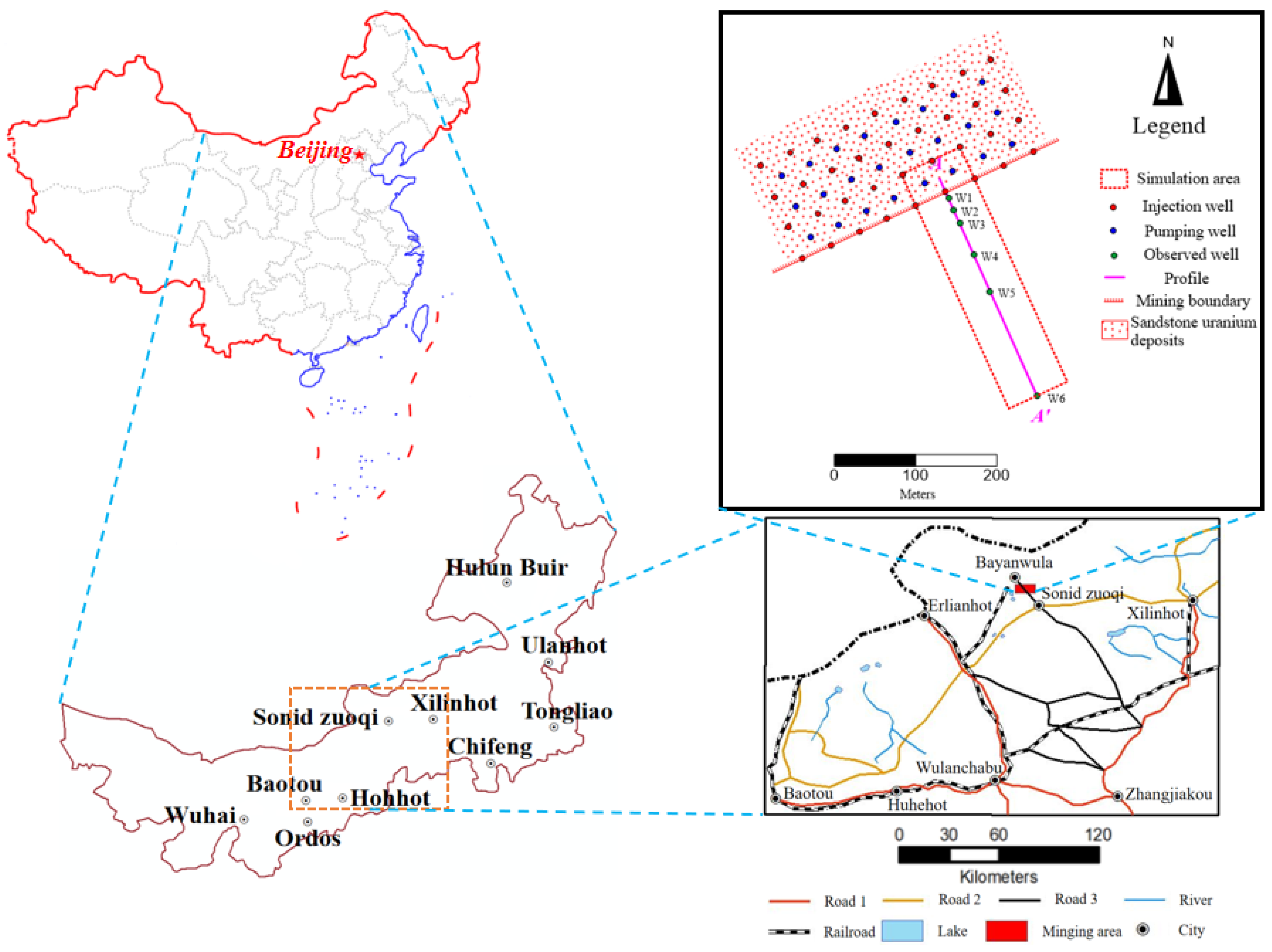
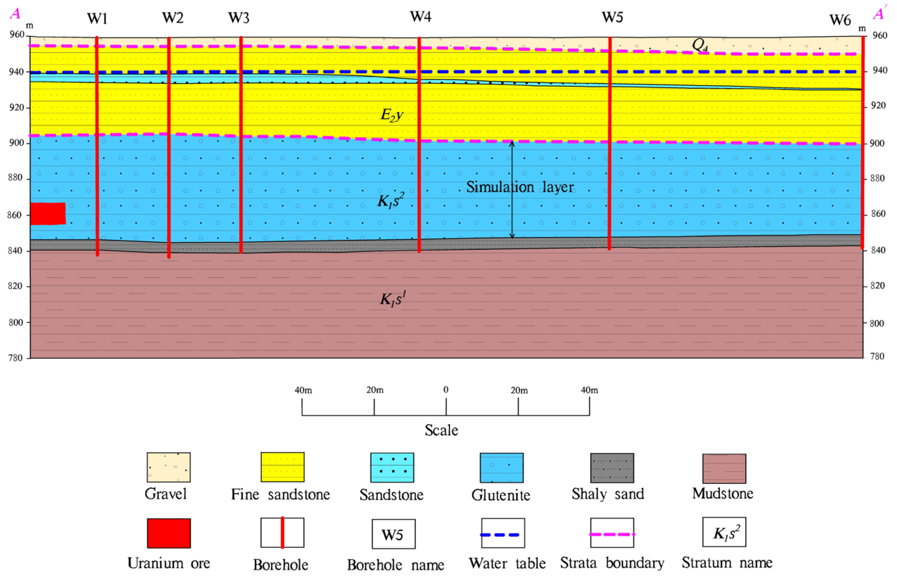
2.1. Geological Environment of the Study Area

(1)

Geology settings

Bayan-Uul mining area is located in the north of the Inner Mongolia Autonomous Region. It is about 30 km to the north of Sonid Zuoqi city. Figure 2 shows the location map and the distribution of boreholes in the mining area.

Figure 3 shows a hydrogeological section of the study area. It can be seen from the figure that the main confined aquifer is located in the upper part of the Saihan Formation (K₁s²), and the aquifer is horizontal. The Irdimanha Formation (E₂y) is distributed at the top of K₁s². It mainly consists of a group of rivers and flood sedimentary sandstone, sand gravel, mud gravel, sand, mud, and rocks. This stratum possesses an approximate thickness of 50 m and serves as the phreatic aquifer. The bottom of Irdimanha Formation (E₂y) as an aquitard of Saihan Formation (K₁s²). The lower part of the Saihan Formation (K₁s¹) is composed of mudstone and silty mudstone mixed with lignite mined in the lake and marsh, and forming a stable aquitard of the aquifer K₁s². The stratigraphic structure is relatively neat. As illustrated in Figure 3, this layer is confined aquifer and primarily composed of sandstone and sandy conglomerate, boasting favorable water yield and permeability characteristics. The estimated thickness of this aquifer is approximately 60 m. According to the survey of the groundwater level, the variation range of the water table is within 0.5 m. The elevation of the water level is around 941 m. The primary aquifers in the study area consist of both the phreatic aquifer (E₂y) and confined aquifer (K₁s¹). The general flow direction of groundwater is from the northeast to the southwest, ultimately discharging in the southern and western areas of the ore deposit.

(2)

Conceptual model

In this study, the scope of the simulated region includes two pumping units. To study the influence of ISL on the outside of the mining area, the simulation area also includes areas outside the pumping unit, which are up to 300 m away from the pumping unit (Figure 4).

2.2. Governing Equations

The governing equation involved in the model is as follows [39]:

(1)

Water flow equation

The equation can be established from the conservation of mass:

$$\frac{\partial M_{\kappa }}{\partial t}=-\nabla F_{\kappa }+q_{\kappa }$$

(1)

For the water phase:

$$F_w=x_{wl}{\rho }_l\overrightarrow{u_l}+x_{wg}{\rho }_g\overrightarrow{u_g},q_w=q_{wl}+q_{wg}$$

(2)

The mass flux of the multi-phase is according to Darcy’s law:

$$\overrightarrow{u_{\beta }}=-k\frac{k_{r\beta }}{{\mu }_{\beta }}\left(\nabla P_{\beta }-{\rho }_{\beta }\overrightarrow{g}\right)$$

(3)

Combined with the mass conservation equation, the reactive transport model can be expressed as:

$$\frac{d\left(\phi S_l{c}_{jl}\right)}{dt}=-\nabla \left(c_{jl}\overrightarrow{u_l}-\tau \phi S_l{D}_l\nabla c_{jl}\right)+{\sum }_{i=1}^N{\nu }_{jn}{r}_n$$

(4)

The parameters in these equations are shown in the

Table 1. The mathematical model parameters.

Symbol	Meaning	Units	Symbol	Meaning	Units
$M_{\kappa }$	$\mathrm{The}\mathrm{total}\mathrm{mass}\mathrm{of}\mathrm{matter}\kappa$	kg	$S$	Saturation	dimensionless
$t$	Time	s	$\phi$	Porosity	dimensionless
$F_{\kappa }$	$\mathrm{Flow}\mathrm{rate}\mathrm{of}\mathrm{matter}\kappa$	m/s	$k$	Absolute permeability	m2
$q_{\kappa }$	$\mathrm{Source}\mathrm{and}\mathrm{sink}\mathrm{of}\mathrm{matter}\kappa$	kg/s	$k_r$	Relative permeability	dimensionless
$w$	Water phase	dimensionless	$\mu$	Viscosity	dimensionless
$c$	Concentration	mol/l	$l$	Liquid phase	dimensionless
$x$	Mass fraction	dimensionless	$g$	Gas phase	dimensionless
$\rho$	Density	kg/m3	$D$	Dispersion	m2
$u$	Velocity of flow	m/s	$r$	Reaction rate	mol·m−2s−1
$\nu$	Stoichiometric number	dimensionless	$j$	$\mathrm{Species}j$	dimensionless
$P$	Pressure	Pa	$n$	$\mathrm{Reaction}n$	dimensionless

.

(2)

Chemical reaction mathematical models

The main chemical reaction mathematical models in the simulation include equilibrium minerals and kinetic minerals. The equilibrium mineral model is:

$${\Omega }_m=K_m^{-1}\prod _{j=1}^{N_c}{c}_j^{{\nu }_{mj}}{\gamma }_j^{{\nu }_{mj}}$$

(5)

where $K_m$ is the equilibrium constant.

The kinetic mineral model is:

$$r_n=\pm k_n{A}_n{\left|1-{\Omega }_n^{\theta }\right|}^{\eta }$$

(6)

where $A_n$ is the specific surface area of the mineral, and $k_n$ is the nth parallel mineral precipitation or dissolution reaction rate constant that depends on temperature;

Based on the Arrhenius equation, the correlation between $k_n$ and temperature can be written as:

$$k_n=k_{25}^{nu}exp\left[-\frac{E_a^{nu}}{R}\left(\frac{1}{T}-\frac{1}{298.15}\right)\right]+\sum _i\left\{k_{25}^{i}exp\left[-\frac{E_a^i}{R}\left(\frac{1}{T}-\frac{1}{298.15}\right)\right]\right\}\prod _j{a}_{ij}^{n_{ij}}$$

(7)

where $\prod _{\mathrm{j}}{a}_{ij}^{n_{ij}}$ describes the effect of specific ion activity on the i th parallel mineral precipitation and dissolution reaction.

(3)

Models of mineral dissolution or precipitation

According to the geological condition, the uranium mineral is UO₂. The minerals include Quartz (${\mathrm{S}\mathrm{i}\mathrm{O}}_2$), K-feldspar ($\mathrm{K}\mathrm{A}\mathrm{l}\mathrm{S}{\mathrm{i}}_3{\mathrm{O}}_8$), Na-feldspar ($\mathrm{N}\mathrm{a}\mathrm{A}\mathrm{l}\mathrm{S}{\mathrm{i}}_3{\mathrm{O}}_8$), oligoclase (CaNa₄Al₆Si₁₄O₄₀), Na-smectite (Ca_0.145Mg_0.26Al_1.77Si_3.97O₁₀(OH)₂), Ca-smectite (Na_0.29Mg_0.26Al_1.77Si_3.97O₁₀(OH)₂), illite (K_0.6Mg_0.25Al_1.8(Al_0.5Si_3.5O₁₀)(OH)₂), kaolinite (Al₂Si₂O₅(OH)₂), gypsum (CaSO₄·2H₂O) and anhydrite (CaSO₄), hematite (Fe₂O₃), muscovite (KAl₂(AlSi₃O₁₀)(OH)₂), dolomite (CaCO₃), siderite (FeCO₃), and ankerite (CaMg_0.3Fe_0.7(CO₃)₂). These minerals are also considered in the model. Here we have listed some chemical reactions.

$$2\mathrm{N}\mathrm{a}\mathrm{A}\mathrm{l}\mathrm{S}{\mathrm{i}}_3{\mathrm{O}}_8+{\mathrm{H}}_2{\mathrm{S}\mathrm{O}}_4+9{\mathrm{H}}_2\mathrm{O}\to 2{\mathrm{N}\mathrm{a}}^{+}+{\mathrm{S}\mathrm{O}}_4^{2-}+{\mathrm{A}\mathrm{l}}_2{\mathrm{S}\mathrm{i}}_2{\mathrm{O}}_5{\left(\mathrm{O}\mathrm{H}\right)}_4+4{\mathrm{H}}_4{\mathrm{S}\mathrm{i}\mathrm{O}}_4$$

(8)

$$2\mathrm{K}\mathrm{A}\mathrm{l}\mathrm{S}{\mathrm{i}}_3{\mathrm{O}}_8+{\mathrm{H}}_2{\mathrm{S}\mathrm{O}}_4+9{\mathrm{H}}_2\mathrm{O}\to 2{\mathrm{K}}^{+}+{\mathrm{S}\mathrm{O}}_4^{2-}+{\mathrm{A}\mathrm{l}}_2{\mathrm{S}\mathrm{i}}_2{\mathrm{O}}_5{\left(\mathrm{O}\mathrm{H}\right)}_4+4{\mathrm{H}}_4{\mathrm{S}\mathrm{i}\mathrm{O}}_4$$

(9)

$$\begin{array}{c}2{\mathrm{K}}_{0.5}{\mathrm{M}\mathrm{g}}_{0.25}{\mathrm{A}\mathrm{l}}_{2.3}\mathrm{S}{\mathrm{i}}_{3.5}{\mathrm{O}}_{10}{\left(\mathrm{O}\mathrm{H}\right)}_2+\frac{11}{10}{\mathrm{H}}_2{\mathrm{S}\mathrm{O}}_4+\frac{63}{20}{\mathrm{H}}_2\mathrm{O}\\ \to \frac{1}{2}{\mathrm{K}}^{+}+{\mathrm{M}\mathrm{g}}^{2+}+{\mathrm{S}\mathrm{O}}_4^{2-}+{\mathrm{A}\mathrm{l}}_2{\mathrm{S}\mathrm{i}}_2{\mathrm{O}}_5{\left(\mathrm{O}\mathrm{H}\right)}_4+\frac{6}{5}{\mathrm{H}}_4{\mathrm{S}\mathrm{i}\mathrm{O}}_4\end{array}$$

(10)

$$\mathrm{C}\mathrm{a}{\mathrm{C}\mathrm{O}}_3+{\mathrm{H}}_2{\mathrm{S}\mathrm{O}}_4\to \mathrm{C}\mathrm{a}{\mathrm{S}\mathrm{O}}_4+{\mathrm{C}\mathrm{O}}_2+{\mathrm{H}}_2\mathrm{O}$$

(11)

$$\mathrm{C}\mathrm{a}\mathrm{M}\mathrm{g}{\left({\mathrm{C}\mathrm{O}}_3\right)}_2+{2\mathrm{H}}_2{\mathrm{S}\mathrm{O}}_4\to \mathrm{C}\mathrm{a}{\mathrm{S}\mathrm{O}}_4+{\mathrm{M}\mathrm{g}}^{2+}+{\mathrm{S}\mathrm{O}}_4^{2-}+2{\mathrm{C}\mathrm{O}}_2+{2\mathrm{H}}_2\mathrm{O}$$

(12)

$${\mathrm{H}}_4{\mathrm{S}\mathrm{i}\mathrm{O}}_4\to {\mathrm{S}\mathrm{i}\mathrm{O}}_2+2{\mathrm{H}}_2\mathrm{O}$$

(13)

$${\mathrm{F}\mathrm{e}}_2{\mathrm{O}}_3+{3\mathrm{H}}_2{\mathrm{S}\mathrm{O}}_4\to {2\mathrm{F}\mathrm{e}}^{3+}+{3{\mathrm{S}\mathrm{O}}_4^{2-}+3\mathrm{H}}_2\mathrm{O}$$

(14)

(4)

Relative permeability and capillary pressure calculation model

The calculation model of relative permeability and capillary pressure adopts the Van Genuchten–Mualem model.

2.3. Initial Conditions and Boundary Conditions

(1)

Initial conditions

Based on the field investigation results, the initial temperature of the aquifer has been set as 9 °C, and the initial head is 941 m. In order to obtain the initial concentration of each ion in the aquifer, we conducted a field sampling analysis. The initial concentration of ions is listed in

Table 2. Initial concentration of the groundwater.

Index	Concentration
Temperature (°C)	9
pH	7.226
ORP (mV)	196.1
DO (mg/L)	7.37
Na (mg/L)	495
K (mg/L)	8.46
Ca (mg/L)	76.6
Mg (mg/L)	55.2
SO42− (mg/L)	407
CI− (mg/L)	410
HCO3− (mg/L)	1110
Fe (mg/L)	0.747
U (µg/L)	30.1

. The resulting individual sample analysis results are substituted into the model as the initial concentration. The initial minerals considered in this study include Quartz, K-feldspar, Na-feldspar, oligoclase, Na-smectite, Ca-smectite, illite, kaolinite, uranium, hematite, and calcite. The initial mineral composition of the ore layer can be seen in

Table 3. Initial mineral composition.

Name	Chemical Formula	Initial Mineral Volume Fraction of Ore Body	Initial Mineral Volume Fraction of Surrounding Rock
Quartz	SiO2	0.48686	0.48686
K-feldspar	KAlSi3O8	0.21550	0.21550
Oligoclase	CaNa4Al6Si14O40	0.01134	0.01134
Na-smectite	Ca0.145Mg0.26Al1.77Si3.97O10(OH)2	0.08391	0.08391
Ca-smectite	Na0.29Mg0.26Al1.77Si3.97O10(OH)2	0.02597	0.02597
Illite	K0.6Mg0.25Al1.8(Al0.5Si3.5O10)(OH)2	0.02137	0.02137
Kaolinite	Al2Si2O5(OH)2	0.01520	0.01520
Uraninite	UO2	0.01143	0.00000
Hematite	Fe2O3	0.01880	0.01880
Calcite	CaCO3	0.03320	0.01140

.

(2)

Boundary conditions

In this study, through field investigation, we found that the change in water head is weakly affected by mining at the position 200 m to 300 m away from the mining area. Therefore, according to the water level value of the observation well 300 m away from the mining area, the boundary water head of the model is set to 941 m.

2.4. Source and Sink

We investigated the production data of the mine. According to the survey results, the flow rate of the injection well is 176 m³/d, and the flow rate of the pumping well is 264 m³/d.

In order to determine the chemical composition of liquid of injection wells in the simulation process, the injection well sample were taken from the injection wells. According to the analysis results of the single sample, the concentration of chemical components of injection well is as shown in

Table 4. The concentration of injection well.

Index	Concentration
Temperature (°C)	15.2
pH	0.443
ORP (mV)	227.6
DO (mg/L)	9.12
Na (mg/L)	1950
K (mg/L)	533
Ca (mg/L)	441
Mg (mg/L)	916
SO42− (mg/L)	27,300
CI− (mg/L)	464
HCO3− (mg/L)	35
Fe (mg/L)	1580

.

3. Numerical Model

3.1. Selection of Simulator

Based on the mathematical model, the simulator TOUGHREACT Version2.0 is used to build the numerical model. In this study, a reactive transport of mining area mining has been built. A variety of mineral components and water–rock interactions are involved in the model. TOUGHREACT [40] was developed by introducing reactive geochemistry into the framework of TOUGH2 Version 2 [41]. TOUGHREACT has been applied to simulate a wide range of subsurface hydrological and biogeochemical environments. For example, geothermal systems [42], nuclear waste repositories [43], geologic carbon sequestration [44,45], and environmental remediation [46,47].

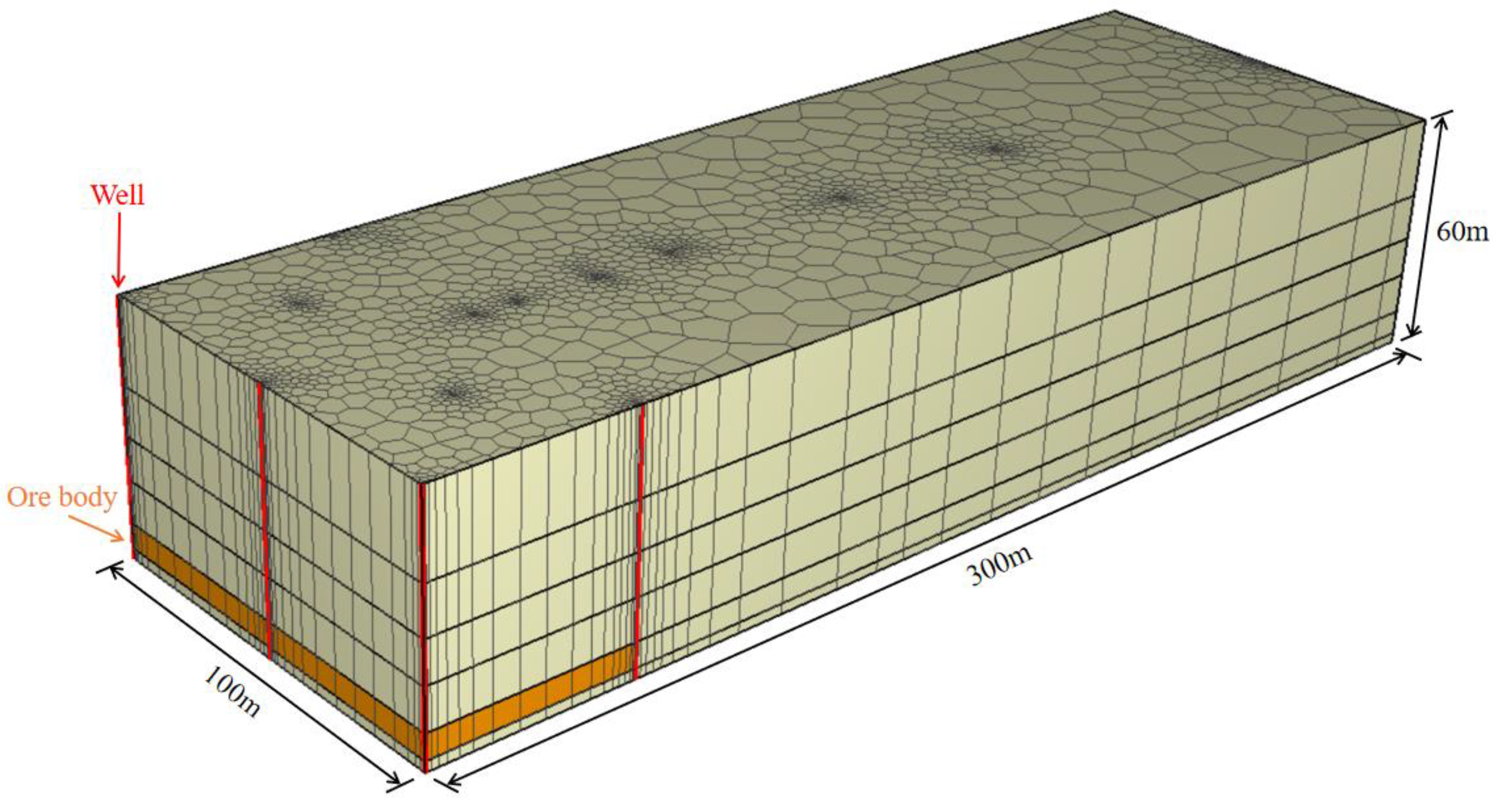
3.2. Mesh Generation

Figure 5 is the mesh structure. According to the simulation area, we have conducted grid division. The grid division ranges from 300 m and 100 m in the horizontal direction and 60 m in the vertical direction. During the model construction process, we encountered the issue of a relatively dense distribution of both extraction wells and injection wells. In order to ensure the accuracy of the simulation near the well, a relatively fine grid is required near the well. At the same time, the number of grids should be minimized to improve computational efficiency. Therefore, we use polygonal grids in the horizontal direction for grid division, and rectangular grids in the vertical direction for grid subdivision. This approach ensures a sufficiently refined grid near the wellbore while controlling the total number of grid. Grid refined is performed near the well. Each layer has 1602 meshes, and the average elements size in the horizontal direction is 18.73 m².

Table 5. The vertical information of grid.

Layer ID	1	2	3	4	5	6
Top elevation (m)	60	40	28.5	18.5	8.5	2.5
Bottom elevation (m)	40	28.5	18.5	8.5	2.5	0
Thickness (m)	20	11.5	10	10	6	2.5

shows the vertical information of grid. The ore body is located on the fifth layer, as shown by the red area in Figure 5.

3.3. The Physical Parameters and the Chemical Reaction Parameters

Based on the regional geological report, the spatial location information of the parameters, and the initial parameter setting of the model for the mineral components information have been confirmed (

Table 6. The aquifer parameters.

Parameters	Value
Aquifer thickness (m)	60
Rock grain density (kg/m3)	2600
Porosity	0.085
K: absolute permeability(m2)	3 × 10−6
Temperature (°C)	9
Rock grain specific heat (J/(Kg·°C))	920
Formation heat conductivity (W/(m·°C))	2.51
Pressure (MPa)	0.1

). The chemical reaction parameters are shown in

Table 7. The mineral reaction kinetic parameters used in the model (the data from the software TOUGHREACT V2.0).

Minerals	Chemical Formula	Surface Area (cm2/g)	Parameters for Kinetic Rate Law
			Neutral Mechanism		Acid Mechanism			Base Mechanism
			k25(mol/ m2/s)	Ea (KJ/mol)	k25(mol /m2/s)	Ea (KJ/mol)	n (H+)	k25(mol/ m2/s)	Ea (KJ/mol)	n(OH−)
Calcite	CaCO3	9.8	Equilibrium
Anhydrite	CaSO4	9.8	Equilibrium
Quartz	SiO2	9.8	1.023 × 10−14	87.7
Illite	K0.6Mg0.25Al1.8(Al0.5Si3.5O10)(OH)2	151.6	1.660 × 10−13	35.0	1.047 × 10−11	23.6	0.34	3.020 × 10−17	58.9	−0.4
K-feldspar	KAlSi3O8	9.8	3.890 × 10−13	38.0	8.710 × 10−11	51.7	0.5	6.310 × 10−22	94.1	−0.823
Chlorite	Mg2.5Fe2.5Al2Si3O10(OH)8	20.0	3.020 × 10−13	88.0	7.762 × 10−12	88.0	0.50
Na-smectite	Na0.29Mg0.26Al1.77Si3.97O10(OH)2	151.6	1.660 × 10−13	35.0	1.047 × 10−11	23.6	0.34	3.020 × 10−17	58.9	−0.4
Kaolinite	Al2Si2O5(OH)4	23.0	6.918 × 10−14	22.2	4.898 × 10−12	65.9	0.777	8.913 × 10−18	17.9	−0.472
Ca-smectite	Ca0.145Mg0.26Al1.77Si3.97O10(OH)2	151.6	1.660 × 10−13	35.0	1.047 × 10−11	23.6	0.34	3.020 × 10−17	58.9	−0.4
Gypsum	CaSO4	9.8	1.6218 × 10−7
Pyrite	FeS2	12.9			2.52 × 10−12	56.9	−0.5	2.8184 × 10−5	56.9	0.5(n(O2(aq)))
Oligoclase	CaNa4Al1.77Si3.97O10(OH)2	10.0	1.4454 × 10−13	69.80
Hematite	Fe2O3	12.9	2.512 × 10−15	66.2	4.0738 × 10−10	66.2	1
Muscovite	KAl2(AlSi3O10)(OH)2	152.0	3.0200 × 10−13	88.0	7.7624 × 10−12	88.0	0.5	3.0200 × 10−13
Siderite	FeCO3	10.0	1.26 × 10−9	62.76	6.46 × 10−4	36.1	0.5
Dolomite	CaMg(CO3)2	12.9	2.52 × 10−12	62.76	2.34 × 10−7	43.54	1
Ankerite	CaMg0.3Fe0.7(CO3)2	9.8	1.26 × 10−9	62.76	6.46 × 10−4	36.1	0.5
Magnesite	MgCO3	10.0	4.5709 × 10−10	23.50	4.1687 × 10−7	14.4	1

.

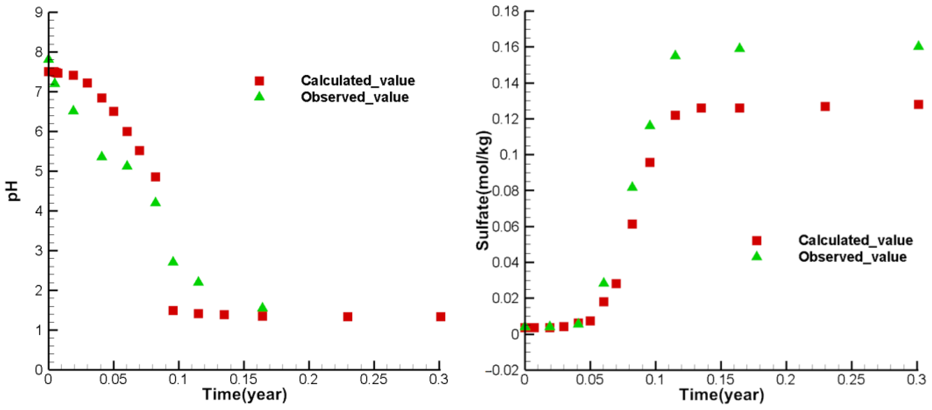
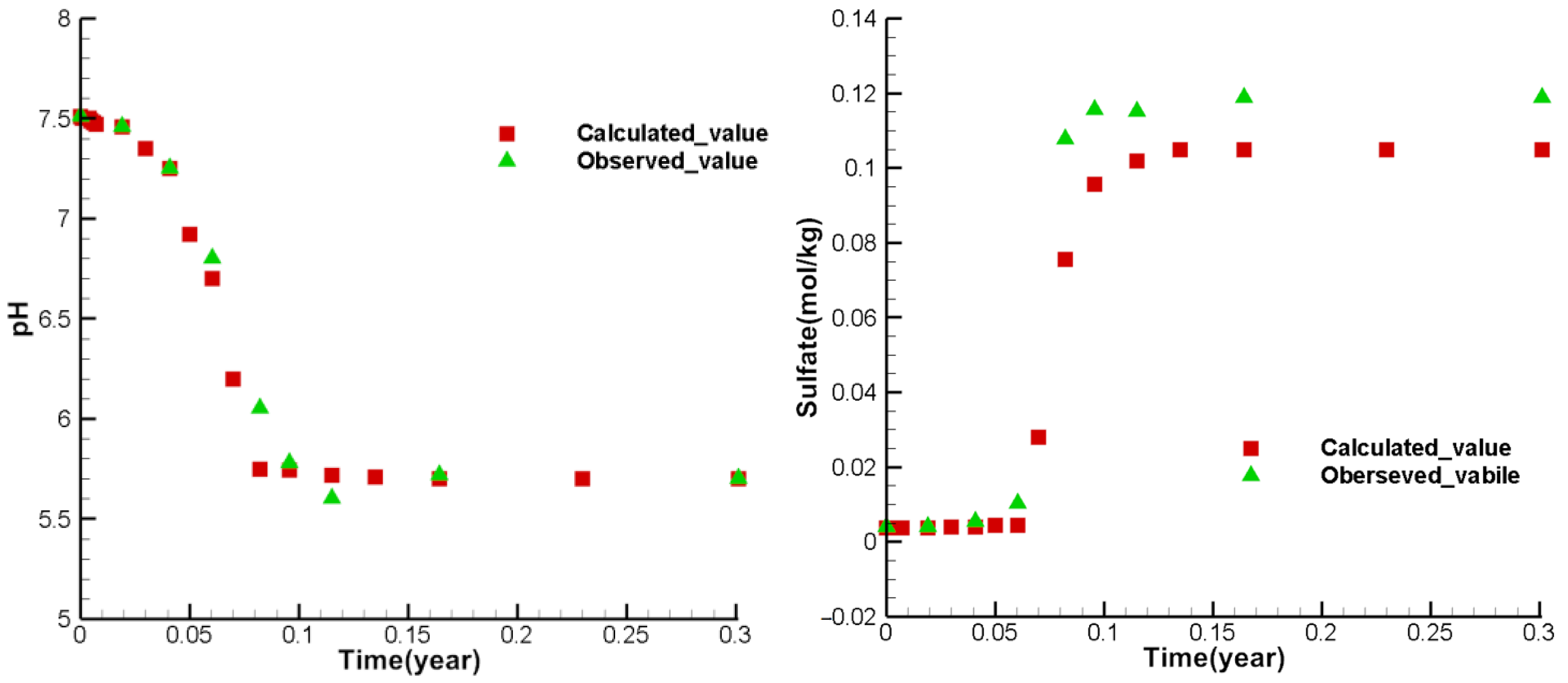
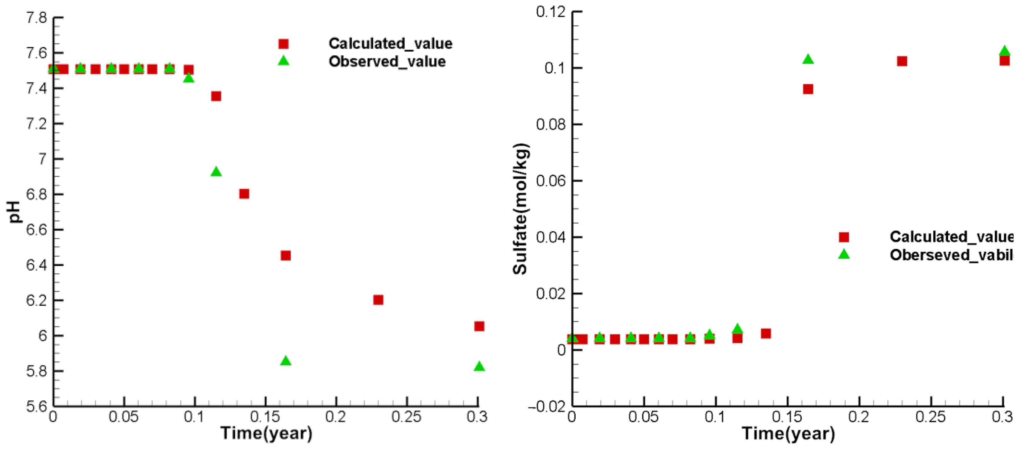
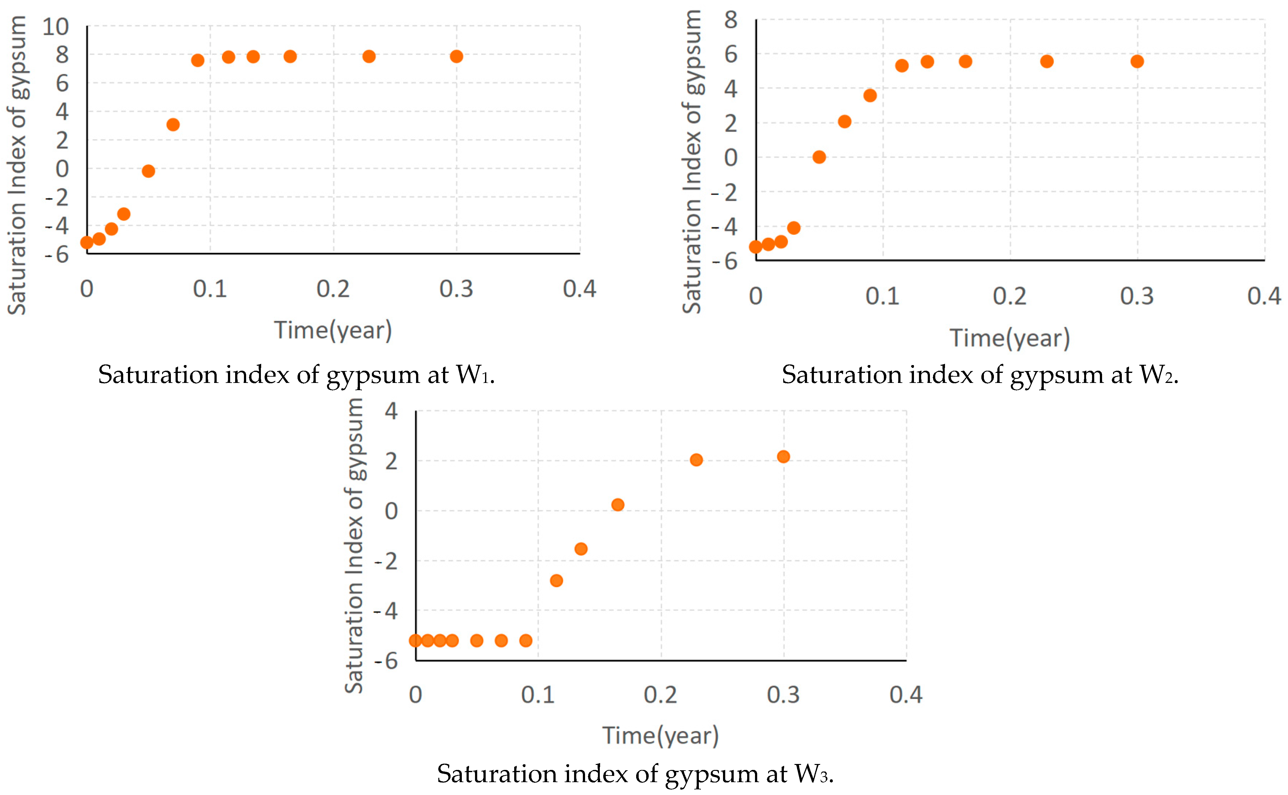
3.4. Model Calibration and Sensitivity Analysis

The linear correlation coefficient is used to characterize the goodness of fit of the model. The coefficient is calculated using the concentration values of different observation wells at different times. The correlation coefficients of the three wells ranged from 0.9433 to 0.9990. The simulation accuracy of this study is above 90%. The expression of the linear correlation coefficient is as follows [48]:

$$r=\frac{{\sum }_{i=1}^n\left(C_i-\overline{C_i}\right)\left(b_i-\overline{b_i}\right)}{\sqrt{{{\sum }_{i=1}^n\left(C_i-\overline{C_i}\right)}^2}\sqrt{{\sum }_{i=1}^n{\left(b_i-\overline{b_i}\right)}^2}}$$

(15)

where $C_i$ is the simulated concentration, $\overline{C_i}$ is the mean value of the simulated value, $b_i$ is the observed concentration, and $\overline{b_i}$ is the mean value of the observed value. Near the simulation area, there are three typical observation holes: W₁, W₂, and W₃. Three observation holes were sampled, respectively. The pH value is for the field test, and SO₄²⁻ was sent to the mining area laboratory for analysis and test.

Figure 6, Figure 7 and Figure 8 show the calibrate points of each test index concentration of each observation well. From the figures, it can be seen that the simulated values of most points are similar to the observed values. The variety trend of the simulated values is consistent with the observed values, indicating that the model can reflect the actual mining and can be used to predict the ISL.

Figure 9 shows the change in the saturation index of gypsum. With the process of ISL, gypsum transform from dissolved state to precipitated state gradually. With the increase in distance between observation well and mining area, the maximum saturation index of gypsum decreases gradually. This is because the concentration of Ca²⁺ and SO₄²⁻ in observation wells close to the mining area is high, and the saturation index peak of gypsum is large.

There are many model parameters for reactive transport, such as activation energy, absolute permeability, and mineral specific surface area. Absolute permeability and mineral specific surface area are two frequently adjusted parameters. We analyzed the sensitivity of the concentrations of H⁺ and SO₄²⁻ with respect to absolute permeability and the specific surface area of different minerals through sensitivity coefficient. Sensitivity coefficient means how much the dependent variable factor is affected by an independent variable factor. The calculation method is a partial differentiation of the dependent variable concerning the independent variable:

$$S_{ij}=\frac{\partial y_i}{\partial x_j}$$

(16)

where $S_{ij}$ is the sensitivity coefficient of the $i$th dependent variable to the $j$th independent variable. In this study, the difference quotient is used instead of the derivative, and the sensitivity coefficient is calculated by the difference quotient.

$$S_{ij}=\frac{y_i\left(x_j+∆x_j\right)-y_i\left(x_j\right)}{∆x_j}$$

(17)

where $y_i$ represents the concentration value of the $i$th index, $x_j$ represents the $j$th dependent variable, and $∆x_j$ represents the increment of the $j$th dependent variable. In this study, $y_i$ was the concentration when the penetration curve was stable.

Through sensitivity analysis, the parameter with the most significant influence on the concentration of H⁺ and SO₄²⁻ is obtained. Figure 10a,b show the changes in groundwater pH and sulfate ion concentration at well W₁ with the increase in absolute permeability. When the absolute permeability of the aquifer increases, the pH value of groundwater at W₁ is lower, and the concentration of sulfate ion is higher. This is because the increase in absolute permeability means that the permeability of the aquifer becomes better, and it is easier for the leaching solution to migrate to well W₁. Figure 10c,d show the concentration variation in H⁺ and SO₄²⁻ with different specific surface area of minerals. Six minerals were selected for analysis in this study. The results show that the pH value of groundwater at W₁ is higher with the increase in the specific surface area of six minerals. This is due to the increase in the specific surface area of minerals, which leads to the acceleration of the consumption rate of H⁺. At the same time, when the specific surface area of gypsum, anhydrite, calcite, and dolomite increases, the SO₄²⁻ concentration at W₁ decreases. This is because the increase in the specific surface area of gypsum and anhydrite will accelerate the precipitation rate of SO₄²⁻. At the same time, the increase in specific surface area of calcite and dolomite will increase the dissolution rate of Ca²⁺, thus accelerating the precipitation rate of SO₄²⁻. The increase in the specific surface area of hematite and K-feldspar will lead to the increase in SO₄²⁻ concentration at W₁. This is because the increase in the specific surface area of these two minerals will increase the consumption rate of H⁺, thus reducing the dissolution rate of calcite and dolomite, thereby reducing the precipitation rate of SO₄²⁻.

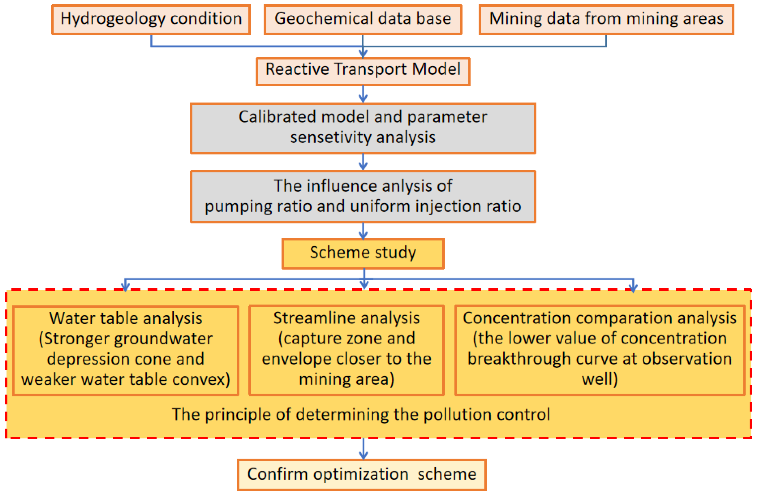
4. Influence of Pumping Ratio and Non-Uniform Injection Ratio of ISL on Groundwater Quality and the Scheme Study

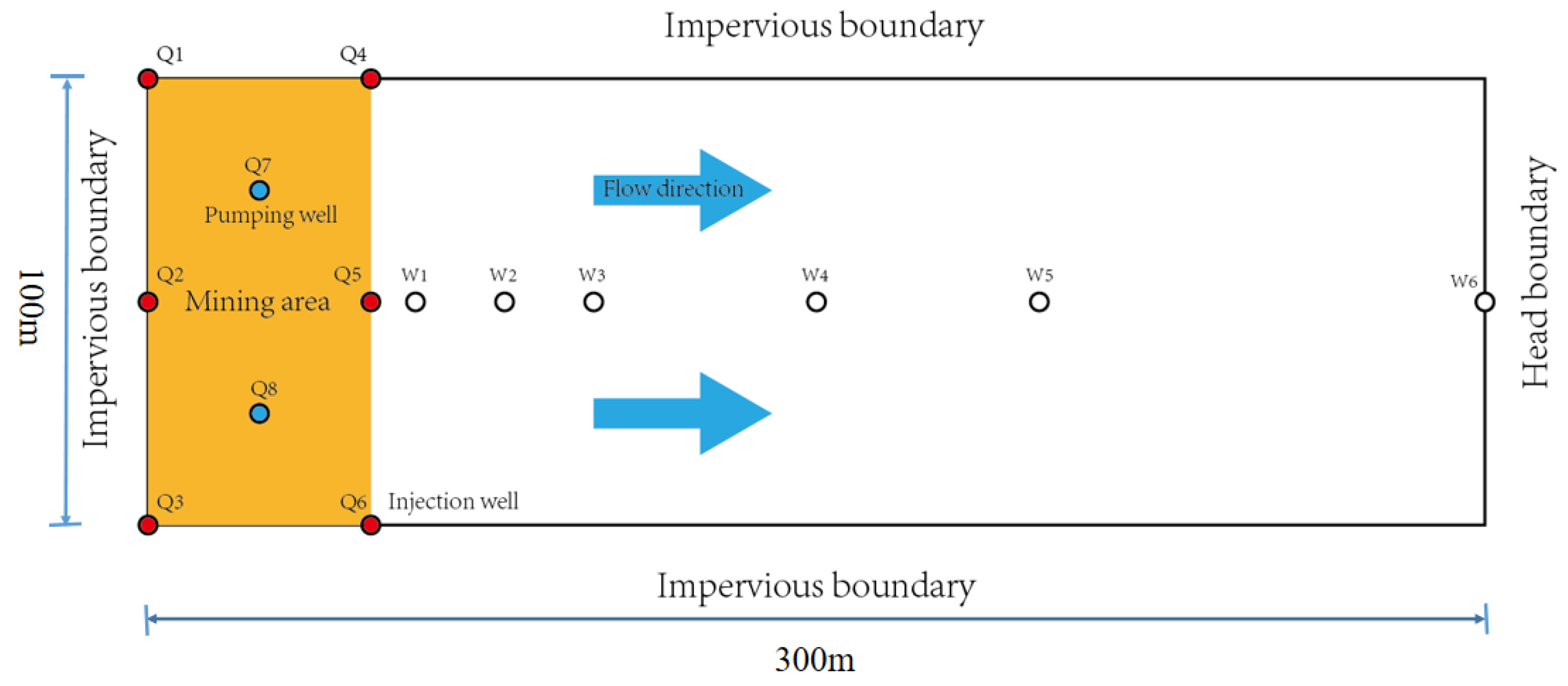
In in situ leaching (ISL), it is crucial to consider the pumping rate and injection rate. These rates should be adequate to fulfill mining requirements, yet not be so large as to cause pollution. Thus, finding the optimal pumping ratio and non-uniform injection ratio is critical. This study conducted a series of scheme studies based on RTM. The RTM accounted for water–rock interactions, resulting in more accurate and reliable results. The numerical simulation method was used to calculate the groundwater dynamic and hydrogeochemical fields in each scenario. A comparative analysis of the water table contour, streamline for each scenario and concentration breakthrough curve at W₁ was conducted to determine the best mining scheme for pollution control.

4.1. Cases Setting

Two factors were considered in this study: one is the pumping ratio, and the other is the non-uniform injection ratio. These two parameters have a significant influence on in situ uranium leaching by controlling the well flux and are easy to realize in actual production.

(1)

Pumping ratio

The pumping ratio is the difference between the flow rate of the pumping well and the injection well, divided by the flow rate of the injection well. For the pumping and injection rate, the pumping ratio can be described as:

$$pumpingratio=\frac{\left({\mathrm{Q}}_7+{\mathrm{Q}}_8\right)-\left({\mathrm{Q}}_1+{\mathrm{Q}}_2+{\mathrm{Q}}_3+{\mathrm{Q}}_4+{\mathrm{Q}}_5+{\mathrm{Q}}_6\right)}{\left({\mathrm{Q}}_1+{\mathrm{Q}}_2+{\mathrm{Q}}_3+{\mathrm{Q}}_4+{\mathrm{Q}}_5+{\mathrm{Q}}_6\right)}$$

(18)

Here, Q₁, Q₂, and Q₃ are the flow rates of the inner injection wells, and Q₄, Q₅, and Q₆ are defined as the flow rates of the outer injection wells. Q₇ and Q₈ are the flow rates of the pumping wells. Their position is given in Figure 3.

According to the characteristics of actual production, we set ${\mathrm{Q}}_1={\mathrm{Q}}_2={\mathrm{Q}}_3={\mathrm{Q}}_4={\mathrm{Q}}_5={\mathrm{Q}}_6$, and ${\mathrm{Q}}_7={\mathrm{Q}}_8$.

(2)

Non-uniform injection ratio

The non-uniform injection ratio is the difference between the flow rate of the injection well in the inner layer of the mining area and that at the edge of the mining area, divided by the flow rate of the injection well at the edge of the mining area. The non-uniform injection ratio is described by:

$$non-uniforminjectionratio=\frac{\left({\mathrm{Q}}_1+{\mathrm{Q}}_2+{\mathrm{Q}}_3\right)-\left({\mathrm{Q}}_4+{\mathrm{Q}}_5+{\mathrm{Q}}_6\right)}{\left({\mathrm{Q}}_4+{\mathrm{Q}}_5+{\mathrm{Q}}_6\right)}$$

(19)

According to the characteristics of actual production, we set ${\mathrm{Q}}_1={\mathrm{Q}}_2={\mathrm{Q}}_3,{\mathrm{Q}}_4={\mathrm{Q}}_5={\mathrm{Q}}_6$, and ${\mathrm{Q}}_7={\mathrm{Q}}_8$.

4.2. Simulation Schemes Design and the Principle of Pollution Control

(1)

Simulation schemes design

Following the analysis of the impact of pumping ratio and non-uniform injection ratio, five schemes have been designed for simulation (scheme 1 to scheme 5). The water level contours and the streamlines are extracted from these models. The contour map of the water level is the fifth-layer grid representing the production zone. The profile of the streamlines has been generated at the central axis. After these numerical simulations, the concentration of UO₂²⁺, SO₄²⁻, and H⁺ at the observation site W₁ was selected for comparative analysis.

Table 8. The simulation schemes.

	Schemes (Simulation Time = 1 Year)
	1	2	3	4	5
Pumping ratio	0	0.01	0.02	0	0
Non-uniform injection ratio	0	0	0	0.05	0.1
Inner injection rate (m3/d) (Q1,Q2,Q3)	176.00	174.24	172.48	184.82	194.09
Outer injection rate (m3/d) (Q4,Q5,Q6)	176.00	174.24	172.48	167.18	158.89
Pumping rate (m3/d) (Q7,Q8)	264.00	265.76	267.52	264.00	264.00

displays the simulation schemes.

(2)

Influence analysis

In order to better understand the influence of pumping ratio and non-uniform injection ratio, an influence analysis was performed for them. The pumping ratio is between 0 and 0.05, the non-uniform injection ratio is between 0 to 1. According to the Formation (18) and Formation (19), the sensitivity is calculated by:

$${\mathit{S}}_{\mathit{i}}=\frac{{\mathit{C}}_{\mathit{i}}-{\mathit{C}}_1}{{\mathit{\xi }}_{\mathit{i}}-{\mathit{\xi }}_1}$$

(20)

where $i$ represents the scheme number, $C_i$ represents the concentration of scheme $i$ at well W₁, ${\xi }_i$ represents the pumping ratio and non-uniform injection ratio of scheme $i$, and $S_i$ is the sensitivity of scheme $i$.

(3)

The principle of determining the pollution control

After determining the above scheme simulation, the better pollution control scheme selection principle of this study is as follows.

(a)

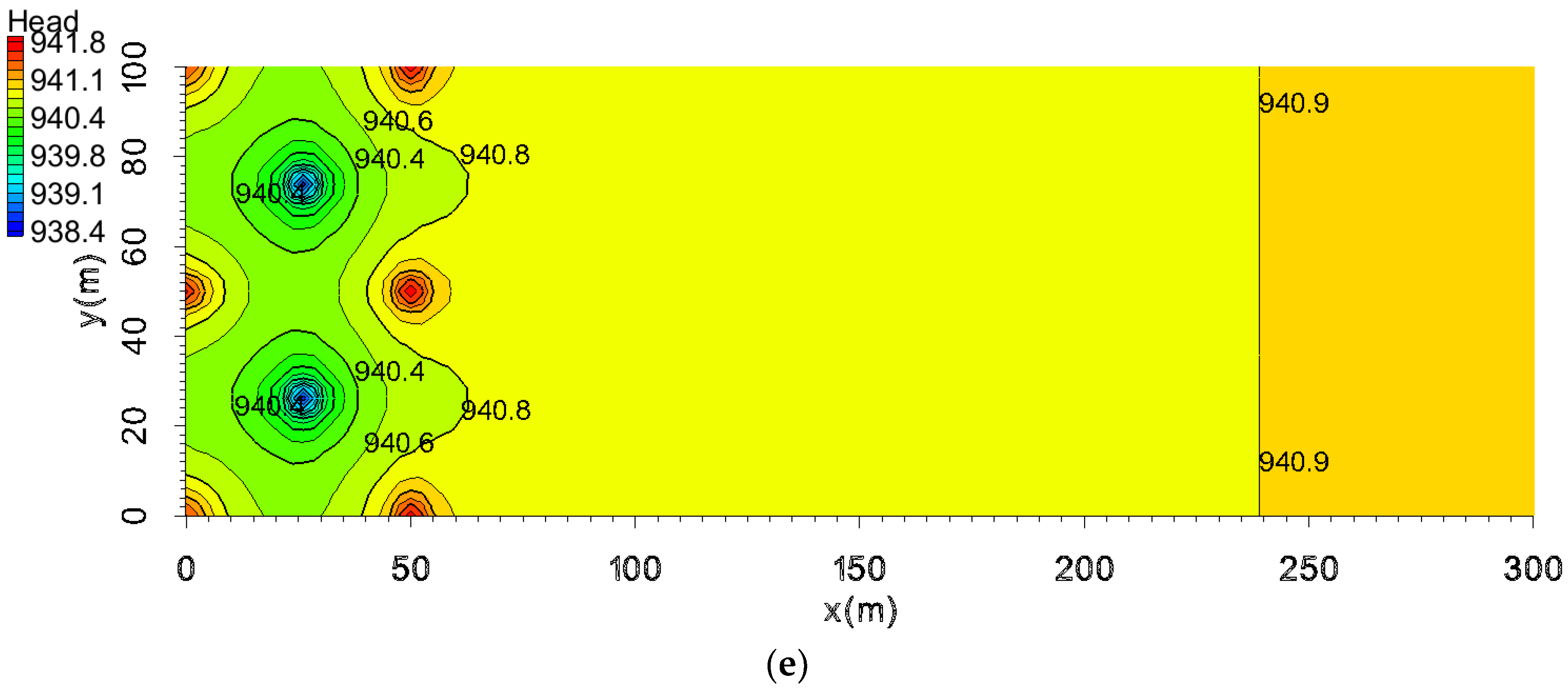
Principle of pollution control based on water level

Based on the numerical simulation results of several schemes, the water table contour map of the mine layer is extracted, respectively. If a scheme has a higher water head outside of the mining area than inside, we believe that this scheme is more optimal.

(b)

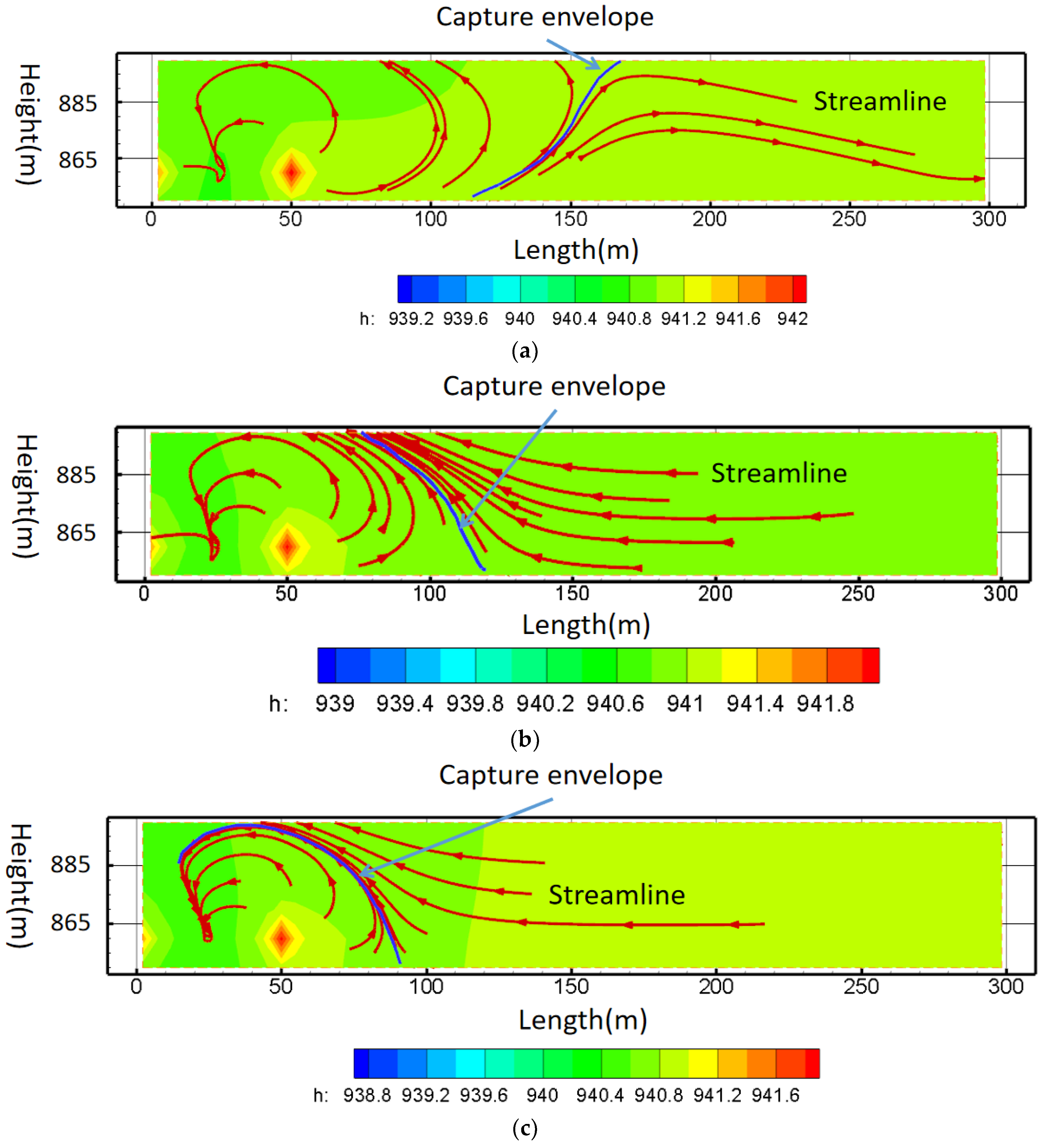
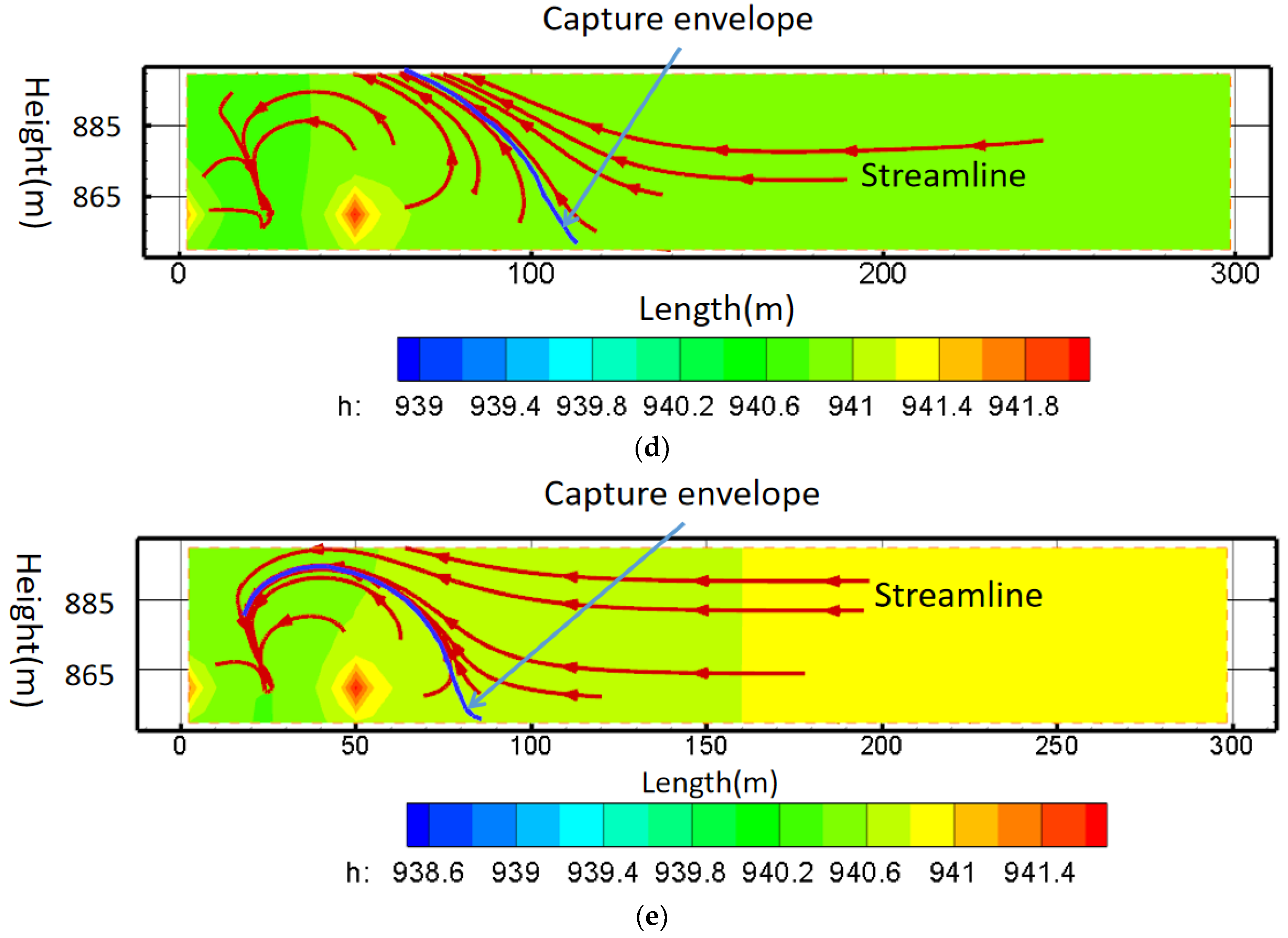
Principle of pollution control based on streamline

The streamline of the vertical section in Q₂-Q₅-W₁-W₂-W₃-W₄-W₅ is analyzed by comparison. The position of Q₂-Q₅-W₁-W₂-W₃-W₄-W₅ is shown in Figure 3. If the characteristics of the streamline back to the mining area are more obvious, this scheme is a better scheme.

(c)

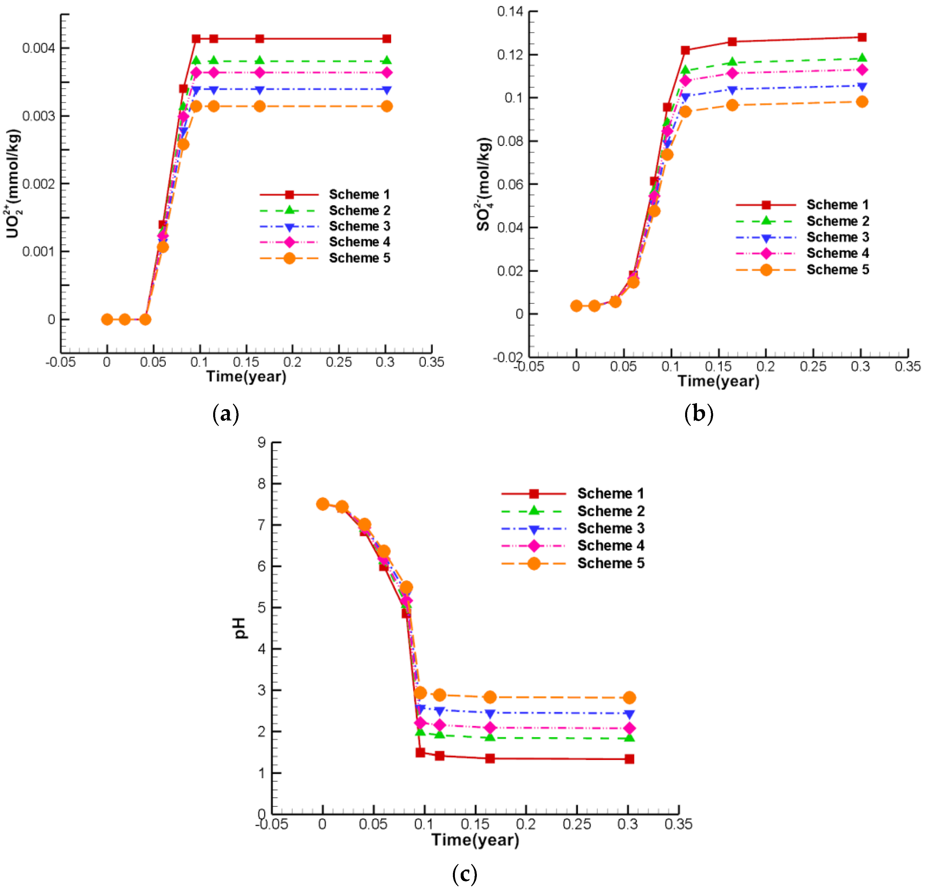
Comparison of concentrations at the observation well W₁

The concentration simulation value of the W₁ observation well, which is most significantly affected by the mining area, is selected for comparison. We considered that the lower the concentration, the more optimal the solution.

5. Results and Discussion

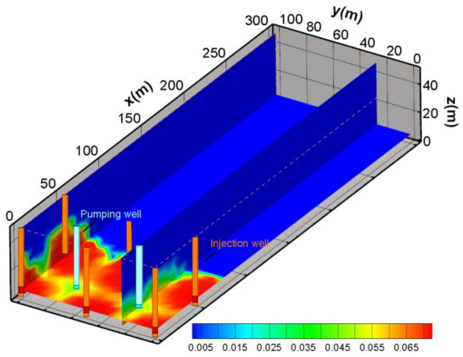
5.1. The Variation in Uranium Ore, UO₂²⁺, SO₄²⁻,H⁺ for Base Scheme (Scheme 1)

(1)

Variation in uranium ore content and migration of UO₂²⁺

When the acid solution is injected into the aquifer, the uranium minerals dissolve in the groundwater, which is the main mechanism of acid in situ leaching. Figure 11 shows the spatial distribution of uranium volume fraction and the UO₂²⁺ concentration after mining for one year. In Figure 11a, the blue area is the uranium dissolution zone, and the red area is the uranium precipitation zone. According to the simulation results, the uranium ore is mainly dissolved near the injection well, which is the main source of UO₂²⁺ in the mining area. Near the injection well, the volume fraction of uranium is reduced to 0.01%. Near pumping wells, the volume fraction of uranium increased to 0.006%. This is because groundwater flows from the injection well to the pumping well, and the sulfuric acid in the leaching solution is consumed gradually, which will cause the pH value to be decreased so that the previously dissolved uranium will be precipitated again. Outside the mining area, the mineral composition does not contain uranium minerals. There is a lack of sources for UO₂²⁺. Consequently, the concentration of UO₂²⁺ is very low in the periphery of the mining area. Figure 11b shown the distribution of UO₂²⁺ concentration. The UO₂²⁺ concentration near the pumping well is higher. The highest concentration of UO₂²⁺ occurs between injection wells and pumping wells. The maximum concentration of UO₂²⁺ can exceed 0.004 mol/kg. The concentration of UO₂²⁺ on the outside of the mining area is relatively low. The concentration front of UO₂²⁺ is about 20 m outside the mining area.

(2)

SO₄²⁻ Spatial distribution characteristics

The concentration spatial distribution of SO₄²⁻ after mining for one year is shown in Figure 12. In the acid ISL process, the amount of sulfuric acid is large. The concentration of SO₄²⁻ is a key indicator that needs to be described. In this simulation, the concentration of SO₄²⁻ is relatively high, with the highest concentration exceeding 0.13 mol/Kg. The maximum migration distance of SO₄²⁻ is more than 150 m. This is mainly because SO₄²⁻ is a large amount of injected ions in mining areas, and its consumption is limited. Although some SO₄²⁻ interacts with minerals, for example, precipitating in the form of gypsum, gypsum is slightly soluble in the groundwater environment of ISL, and therefore, the consumption of SO₄²⁻ is relatively small. For this reason, the concentration of SO₄²⁻ in the injected liquid is too high and the consumption of SO₄²⁻ is very small, which leads to the high concentration of SO₄²⁻ in the groundwater environment of ISL.

(3)

H⁺ spatial distribution characteristics

An important factor affecting ground leaching is H⁺ concentration. Figure 13 shows the variation in pH after one year of mining. At the inside of mine, the pH value is relatively low. The pH value increases gradually with the increase in the distance from the mining area. Figure 13 also shows the situation if the lower pH value range were extended to about 80 m. Figure 14 shows the concentration spatial distribution of H⁺ after one year of mining. The migration amplitude of H⁺ concentration is not as large as SO₄²⁻. This may be due to H⁺ being chemically active, which participates in more reactions and increases consumption during the migration process.

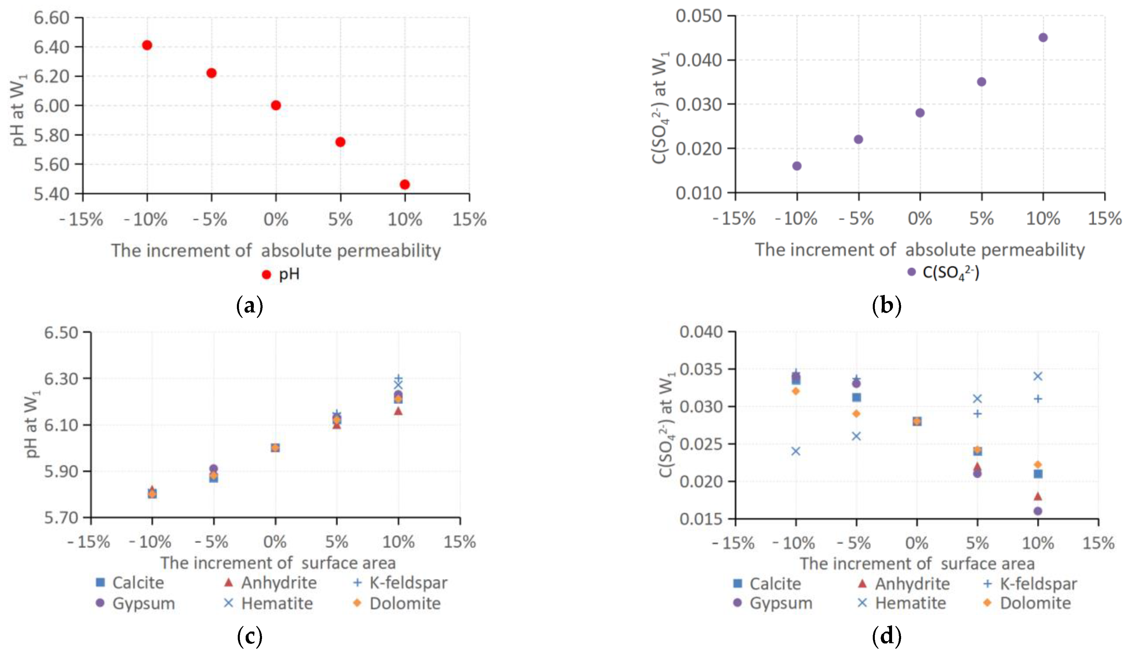
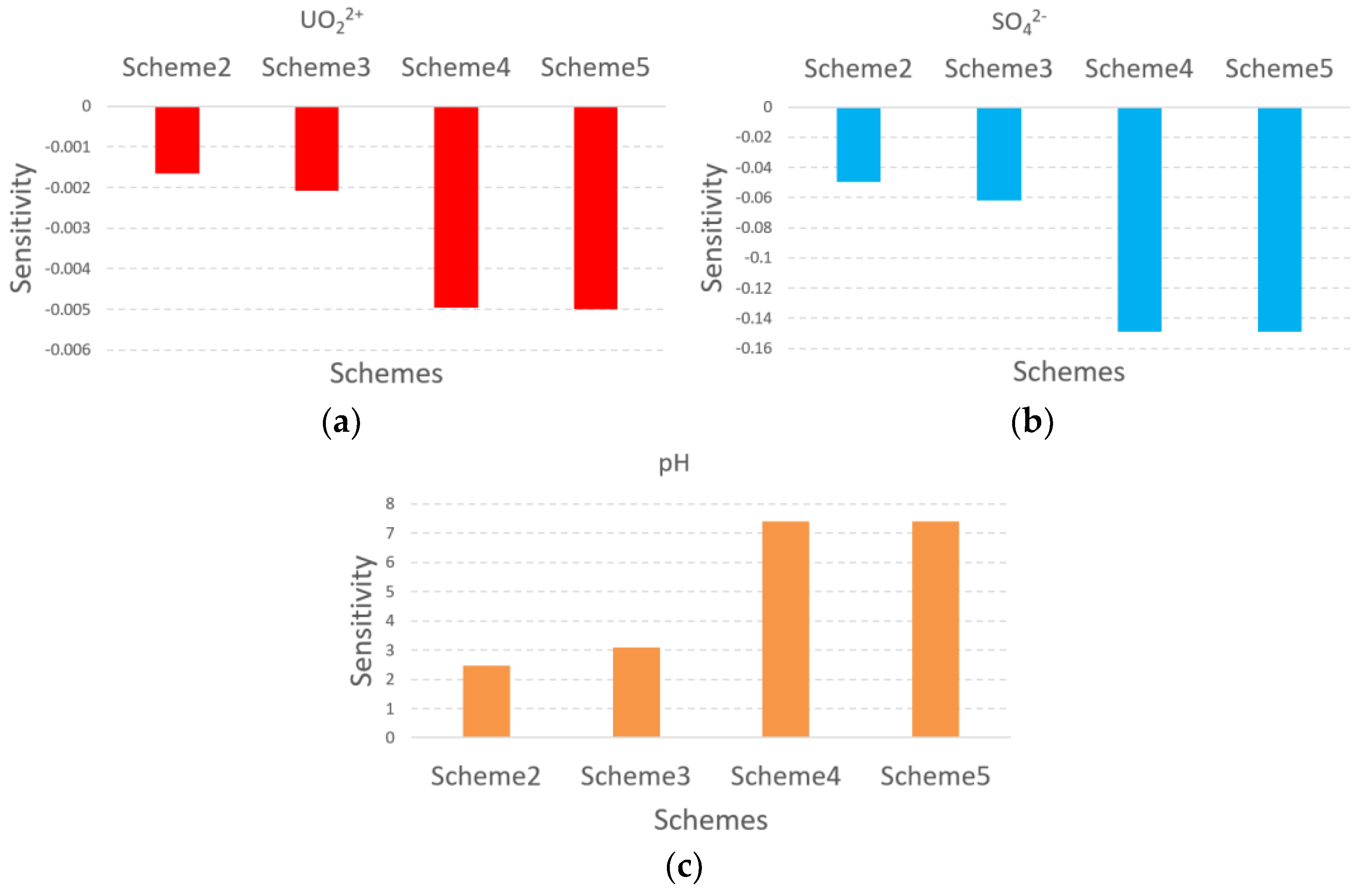
5.2. The Influence of Pumping Ratio and Non-Uniform Injection Ratio for Concentration of UO₂²⁺, SO₄²⁻, and H⁺

We compared the sensitivity of the concentrations of UO₂²⁺, SO₄²⁻, and H⁺ to the pumping ratio (scheme 2, scheme 3) and uniform injection ratio (scheme 4, scheme 5). This was used to measure the influence of different mining schemes on the concentrations of the three ions. In the varying schemes, the concentration of the three ions was derived from numerical simulation results at observation well W₁. Through the influence analysis of the schemes, it can be seen in Figure 15 that using different pumping ratios and non-uniform injection ratio mining schemes, the sensitivity of the concentration values of the three ions is negative. This indicates that these schemes can reduce the concentration of UO₂²⁺, SO₄²⁻, and H⁺ at well W₁. The influence of the non-uniform injection scheme on the concentration of the three ions is greater than the increasing pumping ratio. This indicates that the non-uniform injection scheme has a more significant impact on the concentration of UO₂²⁺, SO₄²⁻, and H⁺ and on pollution control. At the same time, Scheme 5 is a better choice because the concentration of UO₂²⁺, SO₄²⁻, and H⁺ at W₁ in this scheme is the lowest. Therefore, the beneficial impact is strongest. In this scheme, the non-uniform injection ratio is 0.1. The inner injection rate is 194.09 m³/d, the outer injection rate is 158.89 m³/d, and the pumping rate is 264.00 m³/d.

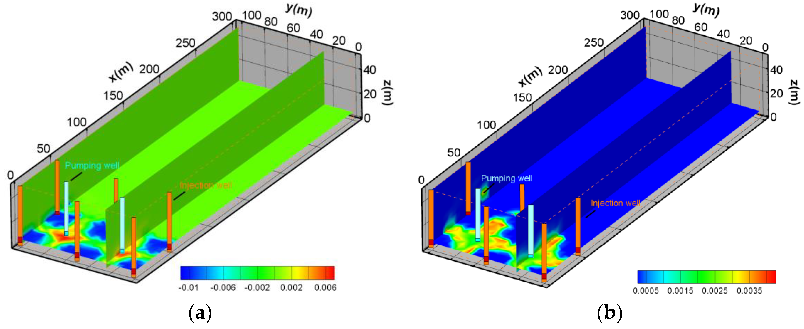
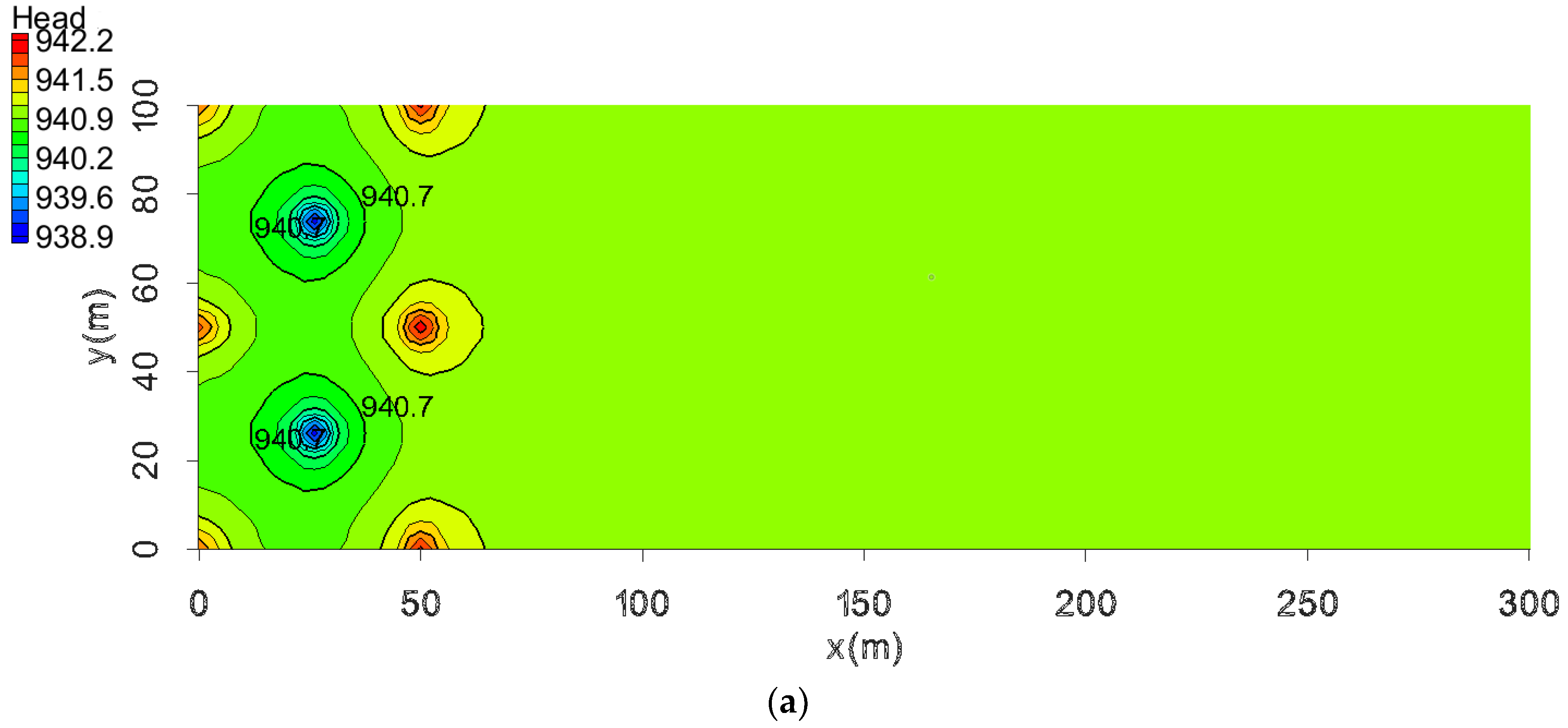
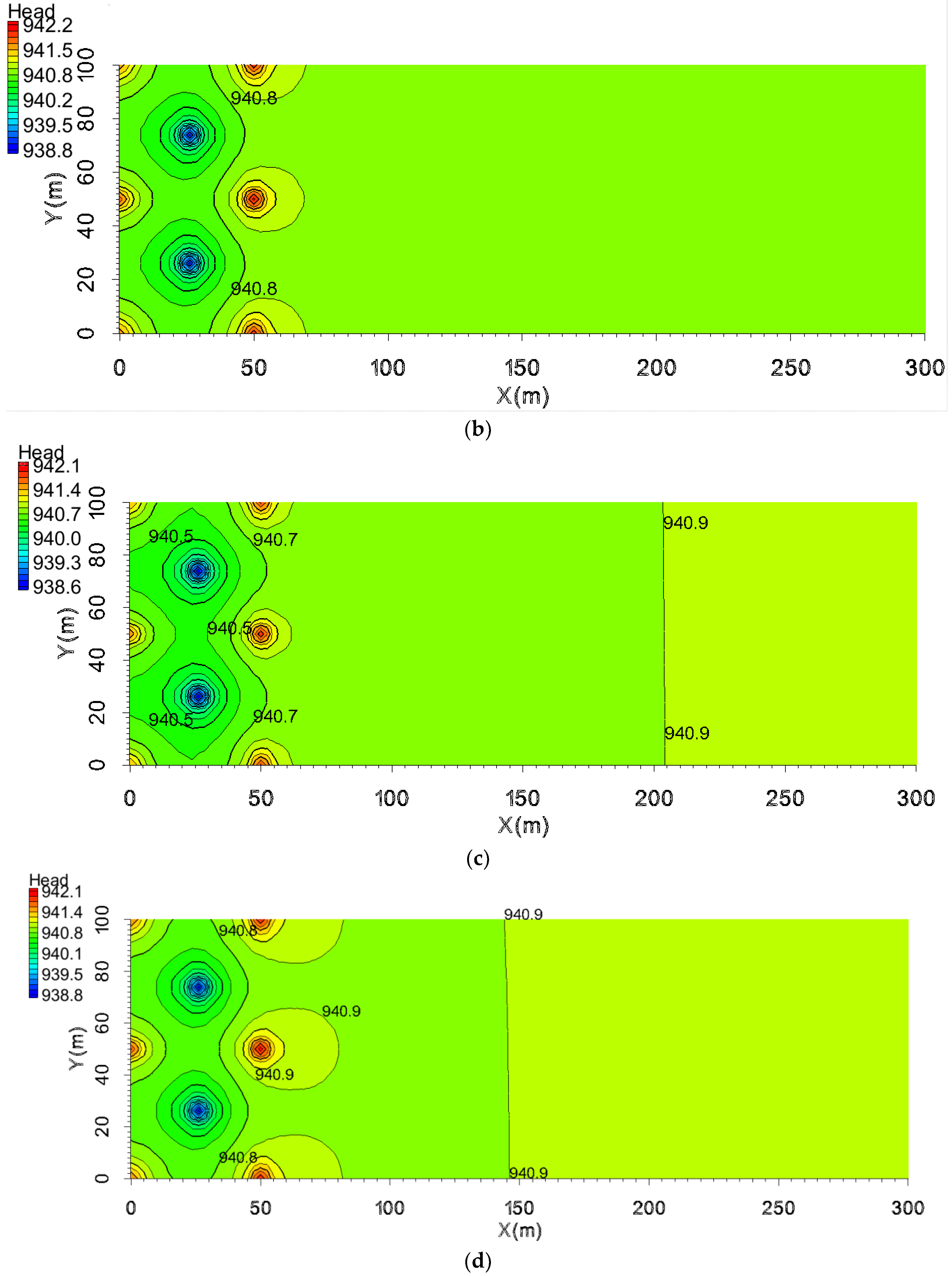
5.3. The Pollution Control Results Based on the Water Table

A contour analysis of the water table changes from scheme 1 to scheme 5 after mining for one year has been performed (Figure 16). Because the head near the injection well was elevated, the water table contours appeared convex. In addition, due to the head near the pumping well being reduced, the water table contours appeared as a groundwater depression cone. Near the mining well, the formation of a groundwater depression cone will cause various solutes in the groundwater to migrate towards the interior of the mining area. The formation of a water table convex will cause these solutes to migrate towards the exterior. At the same time, the level of water inside and outside the mining area will also cause solutes in the groundwater to flow from a high water level position to low water level position. Figure 16a shows that the head spatial distribution for the pumping ratio is 0 and the non-uniform injection ratio is 0. On the outside of the mining unit, the water level far from the mining area is not higher than the water level near the mining area. Figure 16b shows that the head spatial distribution for the pumping ratio is 0.01 and the non-uniform injection ratio is 0. Due to the pumping ratio not being large enough, the water level is similar to that of scheme 1. Figure 16c shows that the water table for the pumping ratio is 0.02 and the non-uniform injection ratio is 0. With the increase in pumping ratio, the groundwater depression cone is strengthened, and the water table convex is weakened. Concurrently, as mining operations advance, the groundwater level in the peripheral regions of the mining area exhibits the following pattern: the groundwater level of the position far from the mining area surpasses that groundwater level of the position nearer the mining area. This characteristic of the groundwater level exerts a notable retarding influence on the migration of pollutants from the inner regions of the mining area to its outer boundaries. Figure 16d shows that the water table for the pumping ratio is 0 and the non-uniform injection ratio is 0.05. With the increase in the non-uniform injection ratio, the influence of groundwater depression cone is strengthened, and the water table convex at the injection wells Q₄, Q₅, and Q₆ is weakened. In the outer area of the mining area, the water level far away from the mining area is higher than the water level near the mining area. Similarly, in the outer region of the mining area, the water level far from the mining area is higher than the water level near the mining area. Figure 16e shows that the water table for the pumping ratio is 0 and the non-uniform injection ratio is 0.1. Under this condition, the water table convex at the injection wells Q₄, Q₅, and Q₆ is weakened more significantly. The groundwater depression cone goes through the gap between Q₄, Q₅, and Q₆, and develops to the outside of the mining area. In the outer region of the mining area, the water level far from the mining area is higher than the water level near the mining area. This characteristic is stronger than that of scheme 3, where the pumping ratio is 0.02 and the non-uniform injection ratio is 0.

Through the comparison of scheme 1, scheme 2, and scheme 3, the water table convex near the outer injection well is weakened with the increase in the pumping ratio. In the area outside the pumping and injection wells, the groundwater level exhibits the characteristic of a high water level on the outside and low water level on the inside. That means that with the increasing of the pumping ratio, the hydrodynamic field is more conducive to preventing pollution migration. Through the comparison of scheme 1, scheme 4, and scheme 5, we know that adopting non-uniform extraction can achieve the same effect as the increase in the pumping ratio. As the non-uniform injection ratio increases and the pumping ratio remains constant, the groundwater level outside the extraction area exhibits a high level on the outer side and a lower level on the inner side. Therefore, the hydrodynamic field formed by increasing the non-uniform injection ratio is also beneficial to preventing pollution migration. The non-uniform injection ratio in scheme 4 is 0.05, and this characteristic is weaker than that in the scheme where the pumping ratio is 0.02 (scheme 3). The non-uniform injection ratio in scheme 5 is 0.1, and this characteristic is stronger than that in the scheme where the pumping ratio is 0.02 (scheme 3). Hence, increasing the non-uniform injection ratio can prevent the migration of pollutants more effectively.

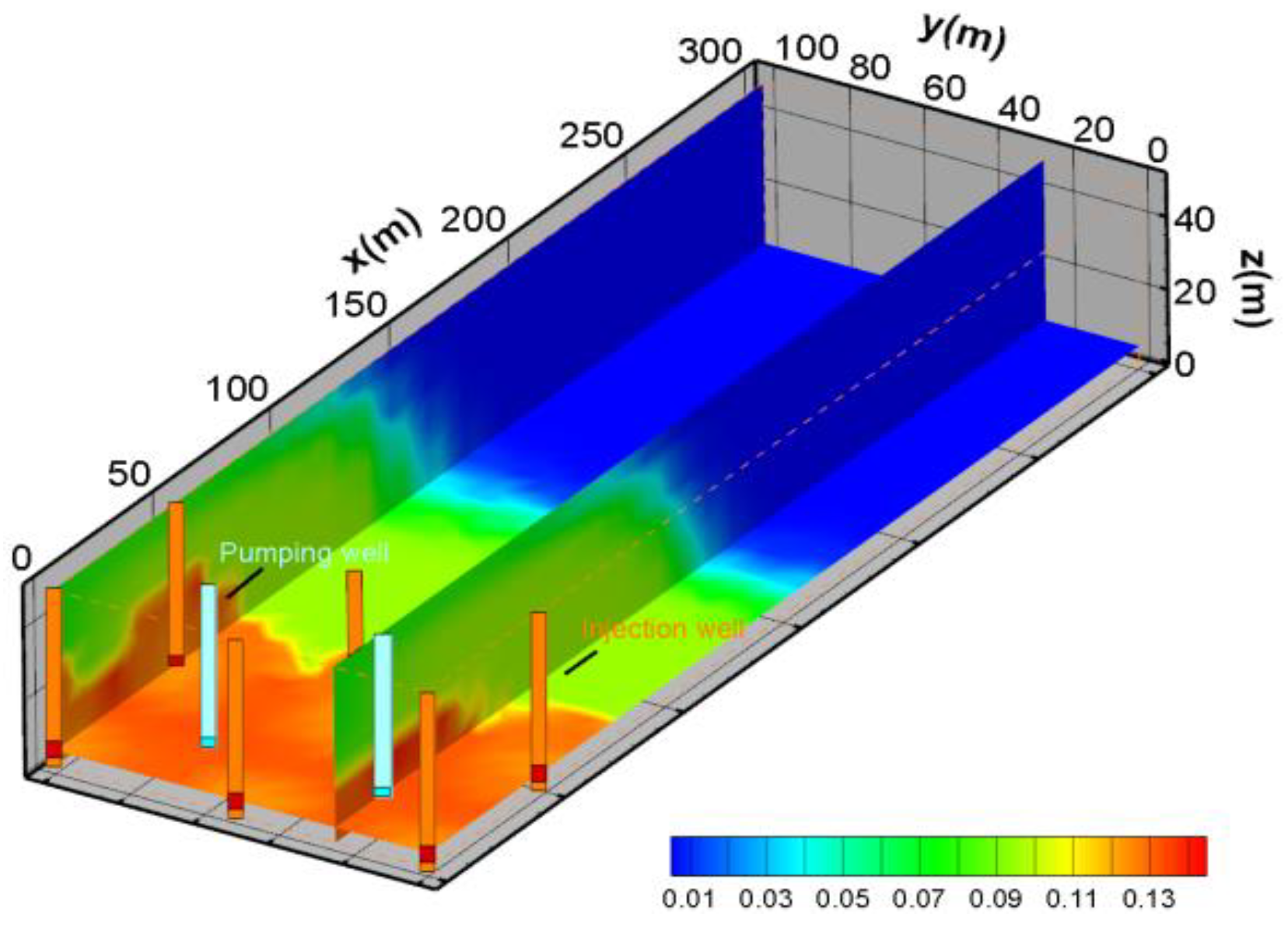
5.4. The Hydrodynamic Pollution Control Results Based on Streamline and Capture Envelope

The characteristics of groundwater streamline can more clearly indicate the direction of solute migration in groundwater. If the groundwater streamline flows from the outside to the inside, it means that the solute in the groundwater will not significantly migrate outward. If the groundwater streamline forms a closed circular structure, it means that the solute in the groundwater can migrate along the flow lines and return to the starting point. We refer to this effect as hydraulic capture. The closed circular streamline area is called the hydraulic capture zone, and the boundary of this area is called the capture envelope. In this study, we should determine the scheme in which the groundwater flow lines are from the outside to the inside and with a more significant hydraulic capture effect. Figure 17 shows the streamline and capture envelope of scheme 1 to scheme 5 after mining for one year. The blue line in the figure represents the capture envelope of the streamline, serving as a boundary for the streamline. On either side of this line, the streamline patterns are different. Figure 17a illustrates the streamline features of scheme 1; notably, a segment of the streamline extends beyond the capture envelope, diverging from the inner region to the outer region. This suggests that when adopting the scheme 1 approach, a portion of the pollutants will escape into the peripheral region along the streamline. Figure 17b–e illustrate the streamline characteristics for scheme 2, scheme 3, scheme 4, and scheme 5, respectively. The streamline for these latter four schemes exhibit a convergent feature from the exterior to the interior outside the capture envelope, marking a notable distinction from the streamline characteristics of scheme 1. This indicates that by increasing the pumping ratio and non-uniform injection ratio, a sealed flow field can be established, confining the groundwater pollutants resulting from mining within the capture envelope. Furthermore, in the region outside the capture envelope, the streamline consistently converges from the exterior to the interior, ensuring no contaminants can escape. If the capture envelope is narrower, we assume a stronger hydraulic containment effect, resulting in better control of groundwater pollutants during mining.

By comparing the streamline characteristics of scheme 1, scheme 2, and scheme 3, it is found that the capture envelope of scheme 3 is closer to the mining area than scheme 1 and scheme 2. This indicates that its hydraulic capture is more effective. Therefore, scheme 3 with a pumping ratio of 0.02 is beneficial to preventing pollution migration. By comparing the streamline characteristics of scheme 1, scheme 4, and scheme 5, the result reveals that the best hydraulic capture occurred in scheme 5. Furthermore, comparing Figure 17c,e, the hydraulic capture of scheme 5 is stronger than scheme 3. Hence, the best scheme for preventing pollution migration is scheme 5 with a pumping ratio of 0 and a non-uniform injection ratio of 0.1.

5.5. The Pollution Control Results of Concentration Characteristics at Well W₁ by RTM

Combined with the above streamline characteristics, the grid of W₁ was selected as an observation point to extract the concentration of several indexes at this grid. Since the injected solution in the mining area contains sulfuric acid, pH and SO₄²⁻ are selected as two important single-factor indexes. UO₂²⁺ is the radionuclide index of groundwater with a high health risk. It is also an important single index. Therefore, the single-factor index focuses on UO₂²⁺, SO₄²⁻, and pH.

Figure 18 shows the variation in the concentrations of UO₂²⁺, SO₄²⁻, and H⁺ at W₁. It can be seen in Figure 18 that scheme 5 has the lowest concentration in different mining schemes. This result suggests that adding the flow rate of the internal injection well (Q₁, Q₂, Q₃) and reducing the flow rate external injection well (Q₄, Q₅, Q₆) can effectively weaken the impact of ISL on the water environment in the surrounding area. The low concentration of UO₂²⁺, SO₄²⁻, and H⁺ in scheme 3 suggests that raising the pumping ratio may also have a similar effect. As the pumping ratio increases, more non-ore groundwater will be extracted. In contrast, the effect of scheme 5 is more significant. This approach is a better choice because it has less of an impact on productivity.

6. Conclusions

In this study, a three-dimensional ISL reaction transport model for the Bayan-Uul mining area was constructed. In the 3D model, for partial penetration wells, the filter section is separately layered and given a flow rate. Through this method, the modeling of partial penetration wells is completed. This simulation considers feldspar minerals, clay minerals, uranium minerals, iron minerals, and secondary minerals related to calcium, magnesium, and iron. The mineral types are abundant, which more realistically describes the hydrogeochemical reactions during actual mining processes.

The model results unveils the spatial distribution characteristics of three indicators (UO₂²⁺, H⁺, SO₄²⁻) after one year of mining, as well as the trends in their concentrations over time at fixed observation wells. The changes in the content of uranium and the migration and transformation of uranium mainly occur within the mining area. During the mining process, the content of uranium does not always decrease or increase, but rather exhibits a spiral-like variation uranium is dissolved near the injection well, and the reduction in the volume fraction of uranium can reach 0.01%. Near the extraction well, some uranium will precipitate again, and the increase in the volume fraction of uranium can reach 0.006%. The maximum concentration of UO₂²⁺ occurs at the location between the injection well and the extraction well, with a maximum concentration slightly higher than 0.004 mol/kg. The concentration of SO₄²⁻ is notably high, with its maximum value slightly surpassing 0.13 mol/kg, observed at the injection well site. SO₄²⁻ progressively migrates outward, with its concentration diminishing as it moves away from the mining area. The furthest extent is approximately 150 m from the mining area. The chemical properties of H⁺ are notably reactive, and H⁺, when entering the groundwater, will interact with various minerals. The concentration of H⁺ within the mining area is relatively high, reaching its peak concentration at the injection well site, which can surpass 0.07 mol/kg. Beyond the mining area, the concentration rapidly diminishes to the background level. Consequently, the migration range of H⁺ is relatively limited, extending up to approximately 80 m from the mining area. Using well W1 as the observation well (10 m from the mining area), the concentration changes in three indicators UO₂²⁺, SO₄²⁻, and H⁺ over a one-year period were monitored. The results indicated that their concentrations began to increase around 0.05 years. After 0.08 years to 0.1 years, they reached a maximum value, and then the concentration values stabilized. Based on the influence analysis of the pumping ratio and non-uniform injection ratio, the non-uniform pumping mode (Scheme 5) proves to be more effective than solely increasing the pumping ratio.

Five schemes controlled by pumping ratio, and a non-uniform injection ratio, were simulated and compared. The simulation results reveal that the greater the pumping ratio and non-uniform ratio, the smaller the migration distance of groundwater pollutants. At the same time, as the pumping ratio gradually increases, a capture zone will form around the mining area. When the pumping ratio increases gradually, a capture zone will be formed near the mining area. The capture zone on groundwater will be more advantageous in preventing the outward migration of groundwater contamination. When the flow rate of the internal injection well increases and the flow rate of the marginal injection well is reduced (the non-uniform injection ratio increased), the capture zone will also be formed near the mining area, preventing the outward migration of groundwater contamination. Through the comparison of the pumping ratio and non-uniform injection ratio, the results show that a non-uniform injection ratio equal to 0.1 is the most beneficial in forming the hydraulic capture zone. In this scheme, the inner injection rate is 194.09 m³/d, the outer injection rate is 158.89 m³/d, and the pumping rate is 264.00 m³/d. The analysis of ion concentrations under various mining conditions indicates that the non-uniform pumping mode can mitigate the impact of acid leaching on groundwater quality.

In summary, this model simulated the reactive transport in ISL. Based on various scenarios, we discussed the optimization of control schemes for groundwater contaminant migration. In the future, we will gradually incorporate adsorption and expand the number of wells to refine the model. The results suggested to combine the non-uniform mining mode in the process of uranium leaching. In this way, the pollution of the groundwater environment caused by in situ uranium leaching can be better controlled.

References

1. Saunders, J.A.; Pivetz, B.E.; Voorhies, N.; Wilkin, R.T. Potential aquifer vulnerability in regions down-gradient from uranium in situ recovery (ISR) sites. J. Environ. Manag. 2016, 183, 67–83. [Google Scholar] [CrossRef] [PubMed]
2. Bhargava, S.K.; Ram, R.; Pownceby, M.; Grocott, S.; Ring, B.; Tardio, J.; Jones, L. A review of acid leaching of uraninite. Hydrometallurgy 2015, 151, 10–24. [Google Scholar] [CrossRef]
3. Wellmer, F.W.; Becker-Platen, J.D. Sustainable development and the exploitation of mineral and energy resources: A review. Int. J. Earth Sci. 2002, 91, 723–745. [Google Scholar]
4. Poole, T.; Bruneton, P.; Fairclough, M.; Schnell, H.; Valter, O. Uranium Resources as Co- and By-products of Polymetallic Base, Rare Earth and Precious Metal Ore Deposits; International Atomic Energy Agency: Vienna, Austria, 2018. [Google Scholar]
5. Tulsidas, H.; Fairclough, M. World Distribution of Uranium Deposits (UDEPO); International Atomic Energy Agency: Vienna, Austria, 2018. [Google Scholar]
6. Edwards, C.R.; Oliver, A.J. Uranium processing: A review of current methods and technology. JOM J. Miner. Met. Mater. Soc. 2000, 52, 12–20. [Google Scholar] [CrossRef]
7. Mudd, G.M. Critical review of acid in situ leach uranium mining: 2. Soviet Block and Asia. Environ. Geol. 2001, 41, 404–416. [Google Scholar] [CrossRef]
8. Zhang, C.; Tan, K.; Xie, T.; Tan, Y.; Fu, L.; Gan, N.; Kong, L. Flow Microbalance Simulation of Pumping and Injection Unit in In Situ Leaching Uranium Mining Area. Processes 2021, 9, 1288. [Google Scholar] [CrossRef]
9. Zhang, C.; Xie, T.T.; Tan, K.X.; Yao, Y.X.; Wang, Y.A.; Li, C.G.; Li, Y.M.; Zhang, Y.; Wang, H. Hydrodynamic Simulation of the Influence of Injection Flowrate Regulation on In-Situ Leaching Range. Minerals 2022, 12, 787. [Google Scholar] [CrossRef]
10. Collet, A.; Regnault, O.; Ozhogin, A.; Imantayeva, A.; Garnier, L. Three-dimensional reactive transport simulation of Uranium in situ recovery: Large-scale well field applications in Shu Saryssu Bassin, Tortkuduk deposit (Kazakhstan). Hydrometallurgy 2022, 211, 105873. [Google Scholar] [CrossRef]
11. Mibus, J.; Sachs, S.; Pfingsten, W.; Nebelung, C.; Bernhard, G. Migration of uranium(IV)/(VI) in the presence of humic acids in quartz sand: A laboratory column study. J. Contam. Hydrol. 2007, 89, 199–217. [Google Scholar] [CrossRef]
12. Kurmanseiit, M.B.; Tungatarova, M.S.; Kaltayev, A.; Royer, J.J. Reactive Transport Modeling during Uranium In Situ Leaching (ISL): The Effects of Ore Composition on Mining Recovery. Minerals 2022, 12, 1340. [Google Scholar] [CrossRef]
13. Yabusaki, S.B.; Fang, Y.; Waichler, S.R. Building conceptual models of field-scale uranium reactive transport in a dynamic vadose zone-aquifer-river system. Water Resour. Res. 2008, 44, W12403. [Google Scholar] [CrossRef]
14. Kohler, M.; Curtis, G.P.; Kent, D.B.; Davis, J.A. Experimental Investigation and Modeling of Uranium (VI) Transport Under Variable Chemical Conditions. Water Resour. Res. 1996, 32, 3539–3551. [Google Scholar] [CrossRef]
15. Zhang, X.; Jiao, C.; Wang, J.; Liu, Q.; Li, R.; Yang, P.; Zhang, M. Removal of uranium(VI) from aqueous solutions by magnetic Schiff base: Kinetic and thermodynamic investigation. Chem. Eng. J. 2012, 198–199, 412–419. [Google Scholar] [CrossRef]
16. Bear, J.; Jacobs, M. On the movement of water bodies injected into aquifers. J. Hydrol. 1965, 3, 37–57. [Google Scholar] [CrossRef]
17. Samani, N.; Zarei-Doudeji, S. Capture zone of a multi-well system in confined and unconfined wedge-shaped aquifers. Adv. Water Resour. 2012, 39, 71–84. [Google Scholar] [CrossRef]
18. Muskat, M. The Flow of Homogeneous Fluids through Porous Media; McGraw-Hill Book Company: New York, NY, USA; London, UK, 1937; p. 306. [Google Scholar]
19. Bear, J. Dynamics of Fluids in Porous Media; Elsevier: New York, NY, USA, 1972; pp. 125–129. [Google Scholar]
20. Zlotnik, V.A. Effects of anisotropy on the capture zone of a partially penetrating well. Groundwater 1997, 35, 842–847. [Google Scholar] [CrossRef]
21. Shan, C. An analytical solution for the capture zone of two arbitrarily located wells. J. Hydrol. 1999, 222, 123–128. [Google Scholar] [CrossRef]
22. Christ, J.A.; Goltz, M.N. Hydraulic containment: Analytical and semi-analytical models for capture zone curve delineation. J. Hydrol. 2002, 262, 224–244. [Google Scholar] [CrossRef]
23. Zhan, H.B.; Zlotnik, V.A. Ground water flow to horizontal and slanted wells in unconfined aquifers. Water Resour. Res. 2002, 38, 1108. [Google Scholar] [CrossRef]
24. Xu, S.; Zhu, X. Hydraulic capture technique for remedy of groundwater contaminated by petroleum and its numerical model. J. Hydraul. Eng. 1999, 1, 71–76. [Google Scholar] [CrossRef]
25. Javandel, I.; Tsang, C.F. Capture-zone type curves-A tool for aquifer cleanup. Ground Water 1986, 24, 616–625. [Google Scholar] [CrossRef]
26. Faybishenko, B.A.; Javandel, I.; Witherspoon, P.A. Hydrodynamics of the capture zone of a partially penetrating well in a confied aquifer. Water Resour. Res. 1995, 31, 859–866. [Google Scholar] [CrossRef]
27. Bair, E.S.; Roadcap, G.S. Comparison of flow models used to delineate capture zones of wells.1.leaky-confined fractured-car bonate aquifer. Ground Water 1992, 30, 199–211. [Google Scholar] [CrossRef]
28. Wang, J.C.; Booker, J.R.; Carter, J.P. Analysis of the remediation of a contaminated aquifer by a multi-well system. Comput. Geotech. 1999, 25, 171–189. [Google Scholar] [CrossRef]
29. Fienen, M.N.; Luo, J.; Kitanidis, P.K. Semi-analytical homogeneous anisotropic capture zone delineation. J. Hydrol. 2005, 312, 39–50. [Google Scholar] [CrossRef]
30. Ahlfeld, D.P.; Sawyer, C.S. Well location in capture zone design using simulation and optimization techniques. Groundwater 1990, 28, 507–512. [Google Scholar] [CrossRef]
31. Hudak, P.F. Numerical modeling assessment of three-gate structures for capturing contaminated groundwater. Environ. Geol. 2008, 55, 1311–1317. [Google Scholar] [CrossRef]
32. Kurmanseiit, M.B.; Tungatarova, M.S.; Royer, J.-J.; Aizhulov, D.Y.; Shayakhmetov, N.M.; Kaltayev, A. Streamline-based reactive transport modeling of uranium mining during in-situ leaching: Advantages and drawbacks. Hydrometallurgy 2023, 220, 106107. [Google Scholar] [CrossRef]
33. Aizhulov, D.; Tungatarova, M.; Kaltayev, A. Streamlines Based Stochastic Methods and Reactive Transport Simulation Applied to Resource Estimation of Roll-Front Uranium Deposits Exploited by In-Situ Leaching. Minerals 2022, 12, 1209. [Google Scholar] [CrossRef]
34. Zheng, H.Q.Y. Site Conditions Experiments for Field Test on In-Situ Leaching and Hydrodynamic Simulation of Uranium in Bayan-Uul; East China University of Technology: Nanchang, China, 2017. [Google Scholar]
35. Chang, Y. Simulation Study on Groundwater Dynamics Control of Leaching Range of in-situ Uranium Well Field; University of South China: Hengyang, Hunan, 2020. [Google Scholar]
36. Chen, Q.Q. Numerical Simulation of In-situ Leaching of Uranium by Acid Method Based on Reactive Solute Transport Theory; East China University of Technology: Nanchang, China, 2020. [Google Scholar]
37. Wang, B.; Luo, Y.; Liu, J.H.; Li, X.; Zheng, Z.H.; Chen, Q.Q.; Li, L.Y.; Wu, H.; Fan, Q.R. Ion migration in in-situ leaching (ISL) of uranium: Field trial and reactive transport modelling. J. Hydrol. 2022, 615, 128634. [Google Scholar] [CrossRef]
38. Wang, B.; Luo, Y.; Qian, J.Z.; Li, J.H.; Li, X.; Zhang, Y.H.; Chen, Q.Q.; Li, L.Y.; Liang, D.Y.; Huang, J. Machine learning-based optimal design of the in-situ leaching process parameter (ISLPP) for the acid in-situ leaching of uranium. J. Hydronal 2023, 626, 130234. [Google Scholar] [CrossRef]
39. Xu, T.; Spycher, N.; Sonnenthal, E.; Zheng, L.; Pruess, K. TOUGHREACT User’s Guide: A Simulation Program for Non-isothermal Multiphase Reactive Transport in Variably Saturated Geologic Media, Version 2.0.; Earth Sciences Division, Lawrence Berkeley National Laboratory University of California: Berkeley, CA, USA, 2012. [Google Scholar]
40. Xu, T.; Apps, J.A.; Pruess, K. Reactive geochemical transport simulation to study mineral trapping for CO2 disposal in deep arenaceous formations. J. Geophys. Res. Solid. Earth 2003, 108, 2071. [Google Scholar] [CrossRef]
41. Pruess, K.; Oldenburg, C.M.; Moridis, G.J. TOUGH2 User’s Guide Version 2; Earth Sciences Division, Lawrence Berkeley National Laboratory University of California: Berkeley, CA, USA, 1999. [Google Scholar]
42. Xu, T.; Spycher, N.; Sonnenthal, E.; Zhang, G.; Zheng, L.; Pruess, K. TOUGHREACT Version 2.0: A simulator for subsurface reactive transport under non-isothermal multiphase flow conditions. Comput. Geosci. 2011, 37, 763–774. [Google Scholar] [CrossRef]
43. Dobson, P.F.; Salah, S.; Spycher, N.; Sonnenthal, E.L. Simulation of water-rock interaction in the yellowstone geothermal system using TOUGHREACT. Geothermics 2004, 33, 493–502. [Google Scholar] [CrossRef]
44. Sonnenthal, E.; Ito, A.; Spycher, N.; Yui, M.; Apps, J.; Sugita, Y.; Conrad, M.; Kawakami, S. Approaches to modeling coupled thermal, hydrological, and chemical processes in the drift scale heater test at Yucca Mountain. Int. J. Rock. Mech. Min. Sci. 2005, 42, 698–719. [Google Scholar] [CrossRef]
45. Spycher, N.F.; Sonnenthal, E.L.; Apps, J.A. Fluid flow and reactive transport around potential nuclear waste emplacement tunnels at Yucca Mountain, Nevada. J. Contam. Hydrol. 2003, 62–63, 653–673. [Google Scholar] [CrossRef]
46. Aradottir, E.S.P.; Sonnenthal, E.L.; Bjornsson, G.; Jonsson, H. Multidimensional reactive transport modeling of CO2 mineral sequestration in basalts at the Hellisheidi geothermal field, Iceland. Int. J. Greenh. Gas. Control 2012, 9, 24–40. [Google Scholar] [CrossRef]
47. Audigane, P.; Gaus, I.; Czernichowski-Lauriol, I.; Pruess, K.; Xu, T.F. Two-dimensional reactive transport modeling of CO2 injection in a saline Aquifer at the Sleipner site, North Sea. Am. J. Sci. 2007, 307, 974–1008. [Google Scholar] [CrossRef]
48. Zheng, C.M.; Bennett, G.D. Applied Contaminant Transport Modeling, 2nd ed.; Wiley-Interscience: New York, NY, USA, 2002. [Google Scholar]
Figure 1. The flow chart of this study.
Water 16 00500 g001
Figure 2. Location map of the mining area with borehole geographical details.
Water 16 00500 g002
Figure 3. Hydrogeological section of the study area.
Water 16 00500 g003
Figure 4. Conceptual model of reactive transport simulation.
Water 16 00500 g004
Figure 5. The 3D structure diagram of mesh.
Water 16 00500 g005
Figure 6. Comparison between observed and simulated values at the observation well W1.
Water 16 00500 g006
Figure 7. Comparison between observed and simulated values at the observation well W2.
Water 16 00500 g007
Figure 8. Comparison between calculated values and observed values at the observation well W3.
Water 16 00500 g008
Figure 9. Comparison of the saturation index of gypsum at the observation well W1,W2,W3.
Water 16 00500 g009
Figure 10. The sensitivity analysis of absolute permeability (a,b) and minerals’ specific surface area (c,d) with respect to the concentration of H+ and SO42− (the minerals include calcite, anhydrite, K-feldspar, gypsum, hematite, and dolomite).
Water 16 00500 g010
Figure 11. (a) Spatial distribution of volume fraction variation in uranium ore body, and (b) the distribution of the concentration of UO22+ (simulation time = 1 year).
Water 16 00500 g011
Figure 12. The concentration spatial distribution of SO42−.
Water 16 00500 g012
Figure 13. The spatial distribution of pH.
Water 16 00500 g013
Figure 14. The spatial distribution of H+.
Water 16 00500 g014
Figure 15. The influence of different pumping ratios and non-uniform injection ratio on the concentration of UO22+, SO42−, and pH at W1 (10 m away from the mining area). (a) UO22+, (b) SO42−, (c) pH.
Water 16 00500 g015
Figure 16. Water table contour map of scheme 1 to scheme 5 (time = 1 year). (a) Water table map of scheme 1; (b) water table map of scheme 2; (c) water table map of scheme 3; (d) water table map of scheme 4; (e) water table map of scheme 5.
Water 16 00500 g016aWater 16 00500 g016bWater 16 00500 g016c
Figure 17. The vertical profile for the streamlines of scheme 1 to scheme 5 (time = 1 year). (a) The vertical section for the streamlines of scheme 1; (b) the vertical section for the streamlines of scheme 2; (c) the vertical profile for the streamlines of scheme 3; (d) the vertical profile for the streamlines of scheme 4; (e) the vertical profile for the streamlines of scheme 5.
Water 16 00500 g017aWater 16 00500 g017b
Figure 18. Variation in UO22+, SO42−, and pH of different pumping ratios and non-uniform injection ratio in the selected grid W1 (the distance between mining area and W1 is 10 m). (a) The concentration variation in UO22+; (b) the concentration variation in SO42−; (c) the value variation in pH.
Water 16 00500 g018