Role of Flexible Operation of a Wastewater Treatment Plant in the Reduction of Its Indirect Carbon Dioxide Emissions—A Case Study

Abstract

The increasing share of renewables in electricity grids comes with a challenge of energy surpluses and deficits, which needs be handled by demand side management (DSM) and storage options. Within this approach, wastewater treatment plants (WWTPs), with flexible energy consumption and production processes and storage units, can contribute to stabilizing the grids and integrating more renewables. In this study, the operation of a real WWTP was optimized by mixed integer linear programming (MILP) to minimize its indirect carbon dioxide (CO₂) emissions. The operation of the WWTP was shown to be flexible in following the CO₂ emission factor of the electricity grid, which was possible with the utilization of the WWTP’s storage units and flexible co-substrate feeding. As a result, by changing only the operational behavior of the WWTP, its indirect CO₂ emissions decreased by 4.8% due to the higher share of renewables in the electricity grid. The CO₂ emissions were shown to decrease further up to 6.9% by adding virtual storage units.

1. Introduction

The 2015 Paris Agreement sets the goal to hold the rise in global average temperature below 2 °C above preindustrial levels. The European Union (EU) and its member states are fully committed to the Paris Agreement and have developed a long-term strategy for the reduction of greenhouse gas (GHG) emissions to achieve a climate-neutral EU by 2050. Within this strategy, power generation would be fully decarbonized by 2050 and more than 80% of the EU’s electricity would be produced by renewable energy sources [1]. After rejoining the Paris Agreement, the United States (US) announced a new target to achieve a 50–52% reduction from 2005 levels by 2030 and set a goal to reach 100% carbon-pollution-free electricity by 2035 [2]. China, currently the world’s largest emitter of CO₂, proposed a long-term mitigation goal of carbon neutrality before 2060 and a greater than 65% reduction in carbon intensity by 2030 from 2005 levels [3]. The share of renewables in electricity generation was projected to increase to almost 30% in 2021, the highest share since the beginning of the Industrial Revolution. China alone is likely to account for almost half of the global increase in renewable electricity generation. It is followed by the US, the EU, and India. Together, they represent almost three-quarters of global solar photovoltaic and wind-based energy [4].

WWTPs account for about 56% of the GHG emissions in the water industry [5]. GHG emissions of WWTPs are categorized as direct and indirect emissions. Direct GHG emissions include methane (CH₄), nitrous oxide (N₂O), and CO₂, which can be biologically produced and emitted in sewers and during wastewater and sludge treatment processes [6,7]. However, these direct CO₂ emissions are usually not included in the GHG balance since they originate from the atmosphere and are considered to be carbon neutral due to their biogenic nature [6,8,9]. Indirect GHG emissions include CO₂, which is mainly produced by the consumption of electricity [6,10]. The carbon footprint of a WWTP includes the total set of direct and indirect GHG emissions and it is reported based on the carbon dioxide equivalent (CO₂e) unit [6,11]. Electricity fuel mix, wastewater treatment technologies, treatment capacity, and quality of influent and effluent water strongly determine the amount of CO₂ emissions of WWTPs [8,12].

WWTPs require large amounts of energy input, mostly as electricity, to process the influent [12]. According to a study [13], WWTPs globally use about 3–5% of electricity. WWTPs in the US have a similar share of 3–4% in total national electricity consumption [14,15], while Beijing WWTPs consume 4–6% of total municipal energy [16]. When the energy consumption share of WWTPs in some European countries such as Sweden, Germany, and Spain was investigated, it decreased to 0.7–1% of national energy consumption [12,17,18]. Although WWTPs’ contribution in global GHG emissions is considered to be marginal, they are still an important contributor [8,12]. This is especially true for developing countries such as China and South Africa, whose growing economies would increase the need for wastewater treatment [12]. Global wastewater production is expected to increase by 24% by 2030 and 51% by 2050 [19]. It is estimated that the electricity required for wastewater treatment will increase by 20% in the next 15 years in developed countries, leading to a significant increase in CO₂ emissions and resource consumption [20]. In another study, energy analysts expect that the energy demand for WWTPs will double by 2050 [21]. A recent study investigated two climate scenarios and predicted that energy consumption of WWTPs would increase due to the decrease in the wastewater influent quality by the end of the century [22]. Therefore, energy consumption of WWTPs should be investigated to decrease GHG emissions [8]. Furthermore, this is also very important regarding the strict emission reduction targets of these countries [1,2,3].

Maktabifard et al. [23] have recently provided a comprehensive overview of GHG mitigation strategies in WWTPs. According to [8,12], studies could be grouped on the basis of the main intervention analyzed: (i) reduction of energy demand, (ii) energy production from wastewater, and (iii) integration of the available renewable sources on site. Authors have either discussed and reviewed energy benchmarking data to provide target parameters to understand how energy was used in the facility or they have discussed and compared different decarbonization strategies [8,20,24,25]. Energy efficiency has received growing attention as the number of WWTPs is growing globally and the effluent quality criteria become stricter [26]. Another area of research that has recently received increasing attention is specific control and operation techniques for energy efficiency and GHG reduction in WWTPs [27]. The review paper of Lu et al. covers aspects like conventional, fuzzy, and model predictive control (MPC) and also optimization of operational strategies. For example, a fuzzy logic controller [28] or MPC [29] has been applied to save energy in the aeration. Optimization of operating parameters has been tackled by several groups, e.g., Kim et al. [30]. However, according to [27], optimization algorithms often face challenges particularly in terms of computation times and optimization approaches for DSM are not covered.

The electricity grids driven by renewable-based energy must handle the fluctuations due to varying weather conditions. Therefore, energy surpluses and deficits must be balanced by DSM and storage options. If energy users can shift energy requirements to the times of day when renewable generation is readily available, they can increase renewable integration and reduce GHG emissions [31]. Consumers that are energetically flexible are well suited to act as demand resources [32]. In this work, “flexible/flexibility” covers the range of operation of the units from complete shut-down to full capacity including partial load behavior. Some studies have focused on DSM of WWTPs. Schäfer et al. developed aggregate management to shift loads and provide a procedure to identify usable aggregates, characteristic values, and control parameters to ensure effluent quality of WWTPs [33]. Follow-up studies that included simulations and field tests were carried out to describe the results of a preselection of aggregates as well as examination and evaluation of operational data leading to relevant key figures for flexible plant operation [34]. The results showed that WWTPs had a significant potential to provide energetic flexibility for the stable operation of energy grids and for further integration of renewable energy sources within the frame of energy transition with their energy generators and consumers. Even for vulnerable components, load shifting was possible with appropriate control parameters and reasonable time slots, without endangering system functionality [33,34]. Seier et al. [35] have assessed the effects of load shifting in the sense of DSM on future residual load smoothing for WWTPs in Germany as a case study. The effects on residual load smoothing were investigated by minimizing WWTPs’ electricity purchase costs on a daily basis. The results showed that German WWTPs had a potential to provide an integration of 120 MW_el of surplus renewable electricity into the grid. The developed methodology has a high potential to be applied to other electricity consumers by adapting their boundary constraints. Musabandesu et al. [36] investigated a WWTP that participated as a demand resource on the wholesale energy market through a proxy demand resource program. The results of testing three load-shifting strategies showed that the plant was able to shift its energy load by modifying select operations without impacting wastewater effluent quality and, therefore, could reduce energy costs through participation in demand resource programs. Simon-Várhelyi et al. [16] investigated an intended operational approach to decrease the energy costs of a WWTP. Wastewater influent was partially stored during the daytime and then purified during the nighttime, when energy prices are lower. This load shifting in the WWTP reduced the operational costs by up to 47%. While the aforementioned studies showed the importance of WWTPs in DSM and their suitability for flexible operation, to the best of the authors’ knowledge, how the CO₂ emissions of WWTPs were affected in this approach has not been investigated yet. Kim et al. [30] employed optimization techniques to determine how the operating conditions of WWTPs could be improved by minimizing both the operating costs and GHG emissions, but this work did not consider DSM or renewable share of the grids. This paper aims to fill this gap with an optimization model of a real full-scale WWTP to investigate the effect of flexible operating conditions on the reduction of the WWTP’s indirect CO₂ emissions by increasing the share of renewable energy in the grid.

2. Methodology

The research presented in this paper was realized within a project that included the optimization of an overall model of a WWTP, a waste incineration plant (WIP), and a district heating system of a German city, Krefeld. This study focuses on only the role of the flexible operation of the WWTP. The paper about the optimization of the WIP model is in progress, but the preliminary results were presented elsewhere [37]. In this section, the WWTP used in this study is presented briefly with a process flow diagram. The development and the structure of the WWTP’s optimization model are explained.

2.1. Study Site

A WWTP located in Krefeld, a major city in Germany, and owned by Krefeld Disposal Company (EGK), has been investigated as the case study in this research. Every day, around 90,000 m³ of wastewater and rainwater passes through the Krefeld WWTP, with a 1.2 million population size equivalent, before being discharged into the river Rhine. Every year, around 12,000 tons of dried sewage sludge and 7 million cubic meters of biogas are produced during the wastewater treatment [38].

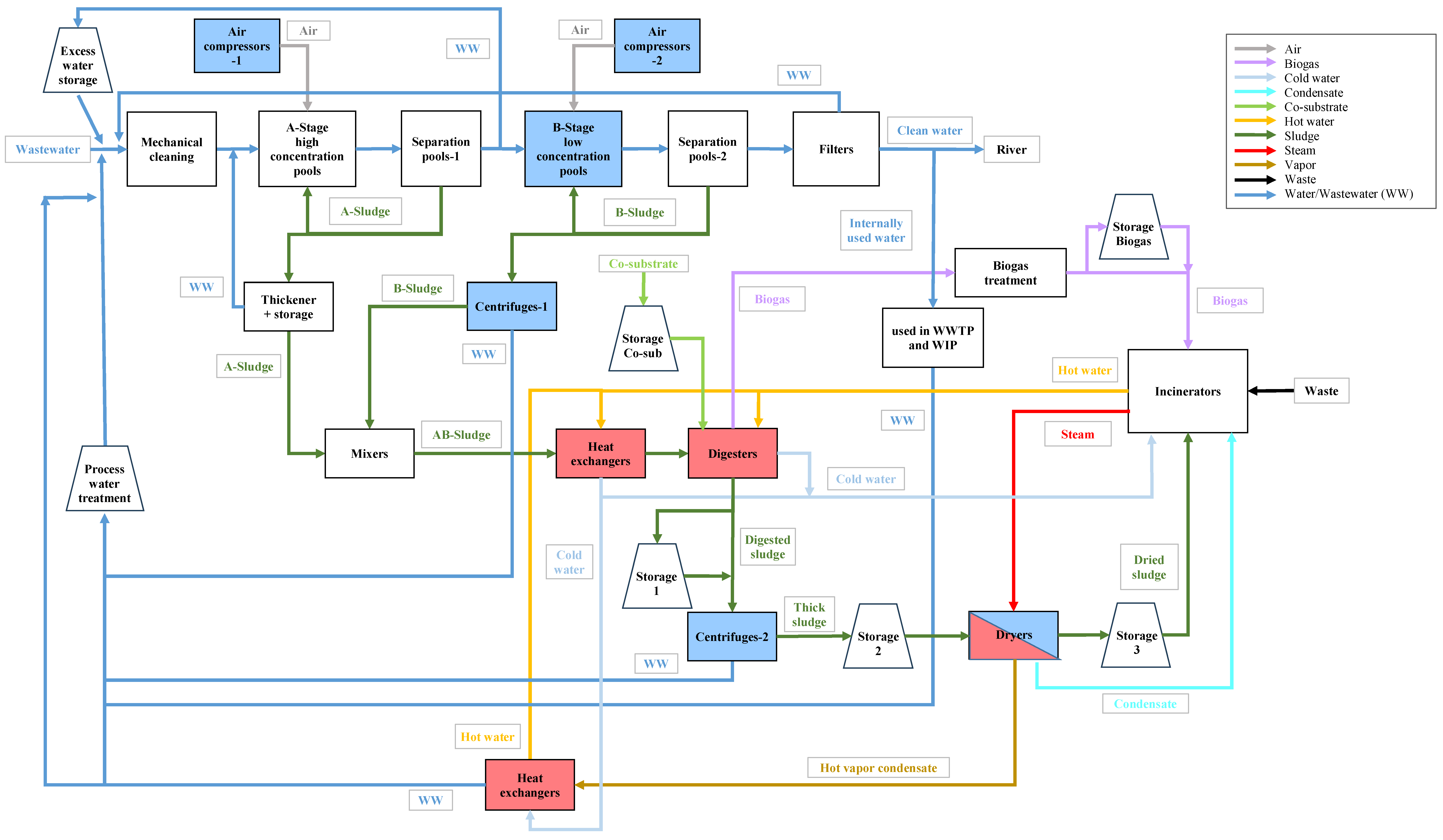
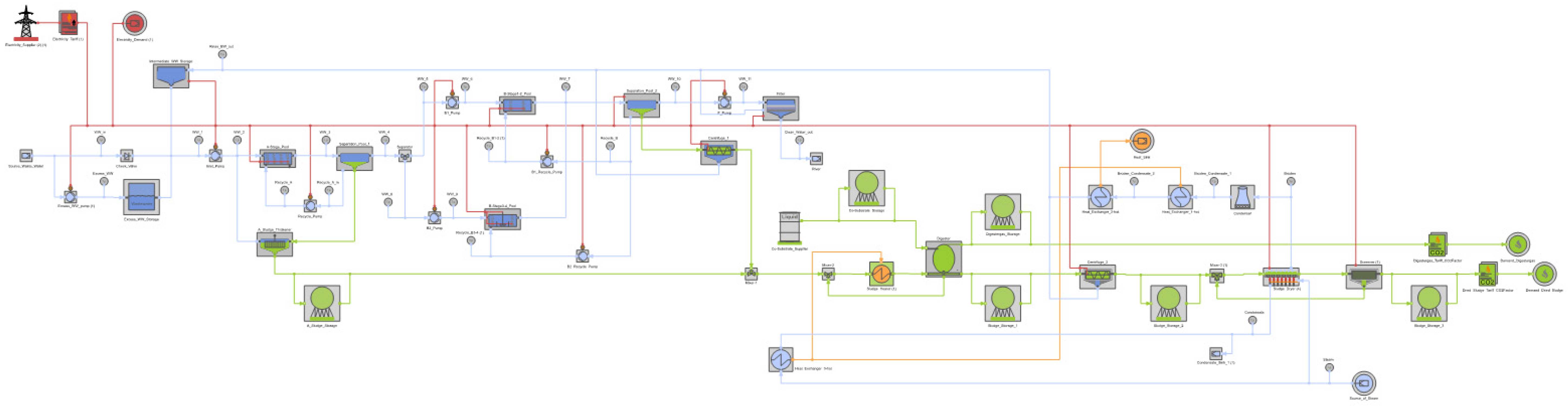
The simplified process flow diagram of the Krefeld WWTP is given in Figure 1, in which parallel unit operations of the same type are shown in one block for a better overview. Firstly, the wastewater is sent to the screeners by the feeding pumps for the mechanical removal of larger solid particles. The WWTP applies a two-stage biological treatment, named the A-B process, to the wastewater [39,40,41]. The wastewater is fed to the high-load activation pools (A-stage), which also include the ventilated sand traps, to decrease its organic content. The A-stage pools may be aerobically or facultatively anaerobically operated to adapt to the wastewater composition. The additional removal of the organic compounds also occurs by adsorption. This decreases the need for air input. The required oxygen (O₂) demand is ensured by the compressed air and nitrate (NO₃). The A-stage achieves high elimination of organic compounds and requires specifically low air input. The wastewater leaving the A-stage pools is sent to the separation pools-1 to separate the A-sludge from the wastewater. Some of the separated A-sludge is recycled back to the A-stage pools to keep a high concentration of bacteria in the A-stage. The excess A-sludge is sent to a static thickener with a storage capacity. The wastewater leaving the separation pools-1 is fed to the low-load activation pools (B-stage) by the intermediate pumps. The B-stage pools serve to eliminate the carbon (C), phosphorus (P), and nitrogen compounds. The required O₂ is supplied from the air compressors. In order to convert the nitrogen compounds into elemental nitrogen (N₂), a corresponding air requirement, which is higher than that of the A-stage, is necessary. The separation pools-2 are downstream of the B-stage pools to separate the B-sludge from the wastewater. Some portion of the B-sludge is recycled back to the B-stage pools and the excess B-sludge is sent to the centrifuges-1. The wastewater leaving the separation pools-2 is sent to the filters for a final clarification. The cleaned water is then discharged to the river, while a portion of it is used internally in the WWTP and the WIP.

Some of the water is removed from the A-sludge in the static thickener, while the dewatering of the B-sludge takes place in the centrifuges-1. Then, the thickened A- and B-sludge streams are mixed in the mixers to produce the AB-sludge. It is preheated in the heat exchangers and fed to the digesters. Also, co-substrates such as waste food and animal fats are fed to the digesters, if available. Anaerobic digestion takes place in the digesters and biogas, which is a mixture of CO₂ and CH₄, is generated as a product. The digested sludge leaving the digesters is sent to the centrifuges-2 and the dryers, respectively, to decrease its water content. The WWTP is integrated into a WIP on the same site, which burns the dried sludge and the biogas produced in the WWTP along with the waste and supplies steam and hot water to the WWTP. The steam is utilized in the dryers to obtain the dried sludge and because of this a vapor stream leaves the dryer. It is condensed and then cooled in the heat exchangers by cold water. The removed heat is used to heat the AB-sludge before being fed to the digesters. Additionally, a hot water stream coming from the WIP is also used to heat the AB-sludge and the digesters when the removed heat from the vapor condensate is not enough. The units with a power demand and/or a heat demand are shown in blue and red, respectively. There are also other units that require power, but only the units with major consumption were considered in this study. Detailed information is given in Section 2.2.

There are several storage options for the sludge, while there is only one storage for the biogas and one for the co-substrate. There is an excess water storage pool (EWP) for the excess incoming wastewater and another process water treatment pool (PWP) to collect the internal streams such as the separated water in the centrifuges and the dryers. The water collected in both pools is then sent to the inlet pumps of the WWTP. The separated water in the thickener is sent to the inlet of the A-stage pools, while the water that was used to rinse the filters is sent to the inlet pumps. A clean water stream, which is separated from the downstream of the filters, is used internally in the WWTP and WIP for different purposes. This water ends up in the process treatment pool after being used.

2.2. Analysis of Electricity Consumption of WWTP

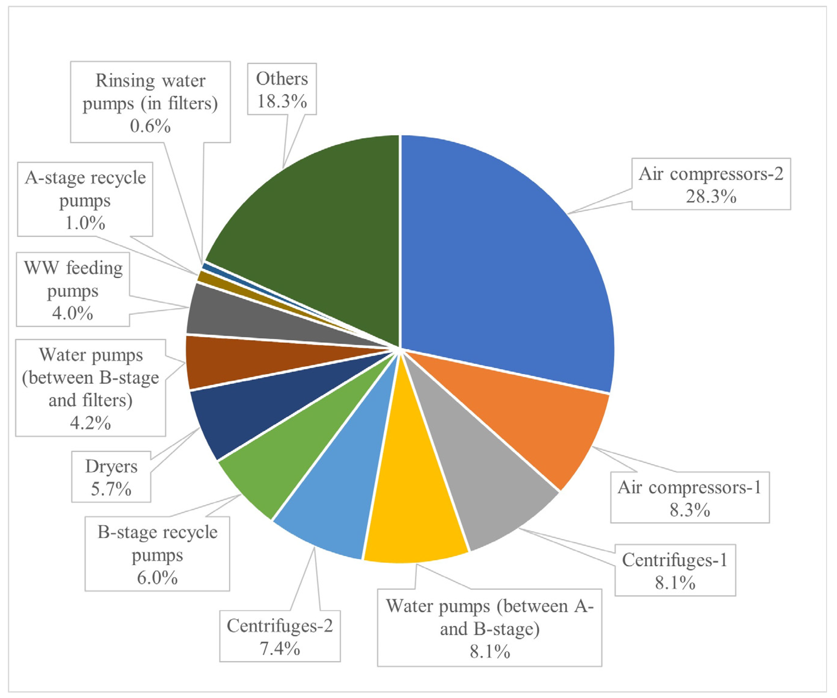
Maximum power demand properties and the total operation hours of the important units of the Krefeld WWTP, whose power consumption was greater than 30 kW, were provided for 2017 by EGK. Based on this information, yearly power consumption values of these units were calculated and ranked (Figure 2). In line with the literature [20,42], air compressors have the highest share in the power consumption chart. The B-stage air compressors have a share of 28.3% and are followed by the A-stage air compressors with a share of 8.3%. The B-stage requires more compressed air than the A-stage due to the characteristics of the processes. The A-stage achieves high eliminations of organic compounds and specifically requires low air input for this. This can be achieved because of the fact that the organic compounds are also removed by adsorption in addition to biological purification. When these air compressors are operated, they consume a large amount of electricity and cause high indirect CO₂ emissions proportionally. If they can be operated at partial loads or shut down completely based on the CO₂ emission factor of the grid, this would cause a dramatic reduction in the CO₂ emissions of the WWTP. So far, promising results have been achieved by theoretical studies and plant-wise operations. Schäfer et al. [33,34] switched off the air compressors of the aeration tanks for several time ranges and examined its effects on the NH4-N effluent concentration. No critical impact on the overall effluent quality was observed for even a 2 h shut-down of the air compressors. Unfortunately, the A-stage compressors cannot be shut down in the Krefeld WWTP since the A-stage pools are also used for sand removal. Shutting off the aeration would result in the settling of mineral particles, which would be very difficult to remove. If a separate sand removal was carried out, then it would be possible to shut down the A-stage compressors.

A-stage air compressors are normally operated on–off in the plant, which means that when they are operated, they work at their maximum capacities regardless of the wastewater inlet. The B-stage air compressors have frequency converters and can be operated at different loads depending on the characteristics of the influent. However, it is not desirable to interrupt the operation of the compressors due to the concerns about the characteristics of the wastewater effluent. The aeration is required to maintain the biological cleaning processes, which is a common concern amongst WWTP operational staff. Another problem that could arise from switching off the aeration [33,34] would be the formation of hydrogen sulfide (H₂S) in both A- and B-stages. This may damage the biology, whose regeneration time can be several weeks. As a result, the wastewater treatment would be severely impaired, and the discharge values could no longer be met [43].

As seen from Figure 2, the water pumps, when summed up, are responsible for 23.9% of the WWTP’s electricity consumption. However, they must also work due to continuous wastewater inlet and lack of storage availability.

Due to the aforementioned reasons, this study focuses mostly on the operational flexibility of the centrifuges-1 and 2 and the dryers, which are the other important power consumers with a total share of 21.2%. Additionally, the A-stage air compressors were assumed to have frequency converters and their power consumption was adjusted to be dependent on the properties of the inlet wastewater. Therefore, the total share of the aggregates in the flexible operation increases to 29.5%. The rest of the plant does not participate in flexible operation.

2.3. Model Assumptions

The creation of the components and the optimization model depends on the following assumptions:

• Only the components whose power consumption is higher than 30 kW were taken into consideration.
• When there is no major heating/cooling in the unit, the inlet temperatures of the units were assumed to be equal to the outlet temperatures.
• The number of most of the units in the WWTP is more than one. They are identical and are operated in parallel. The amount of wastewater incoming to the plant determines how many of them are run simultaneously to meet the capacity. Therefore, each unit was modeled as a single component in the model for simplicity. The properties of each unit such as the flow rates, volumes etc. are added up to define the capacity of a single component. For example, there are two sludge pumps that are operated in parallel, but they are represented in the model by one pump with a total capacity of two pumps. This approach does not interfere with the optimization since the focus is on the total power consumption of the units.
• There is a continuous AB-sludge influent to the digesters of the WWTP because the sludge is fed to the digesters as it is produced. Digested sludge should leave the digesters at roughly the same flow rate as the AB-sludge entering the digesters. So, the digesters were assumed to be operated in a steady state in the model, resulting in continuous biogas and digested sludge production.
• The sludge, the co-substrate, and the biogas (which will be named fuel for the rest of the paper) are biogenic. Due to the fact that their production requires CO₂ captured from the atmosphere, CO₂ from these sources can be considered carbon neutral, as it results in no net GHG emissions or carbon footprint when the fuel is used [9]. CO₂ can be directly emitted by several processes of WWTPs. However, these emissions are not accounted for under the carbon footprint calculations due to their biogenic origin [8]. In this study, only indirect CO₂ emissions coming from the electricity consumption of the WWTP were considered.
• The A-stage air compressors were assumed to have frequency converters and their power consumption was adjusted to be dependent on the mass flow rate of the inlet wastewater (except the WWTP-REF model in Section 3.2).

2.4. Optimization Problem

The optimization problem is explained in detail in this section. The goal was to optimize the WWTP operation for a meaningful period of at least several days in an hourly resolution.

2.4.1. Optimization Model

The optimization model of the Krefeld WWTP was developed in TOP-Energy 2.9, a commercial software for mixed integer linear optimization of energy systems [44]. All unit operations in TOP-Energy 2.9 are written in a language that is similar to the Modelica modeling language, which is used for modeling, simulation, and programming of physical and technical systems and processes [45]. Some of the components of the WWTP model such as water pumps, fuel storage units, mixers, and separators were used directly from the TOP-Energy 2.9 software library. The main components of the WWTP such as various pools, centrifuges, water storage units, dryers, and digesters are not available in the library. Therefore, they were created by using the TOP-Energy 2.9 Template Editor. GUROBI, a commercial MILP solver, was used in the optimization.

In optimization of energy systems, MILP is often used [46,47,48] because nonlinear optimization models are computationally too demanding and not guaranteed to find the global optimum [49]. This is especially true if many time steps are involved. However, because of its restriction to linear equations, MILP requires simplifications that are explained in the following subsections. Essentially, most variables except for the optimization variables—mass and energy flow rates—have fixed values. These values can either be set as fixed parameters or calculated from nonlinear model equations before the actual optimization. For many components in energy systems, this is not a severe limitation because energy vs. mass flows are indeed close to proportional.

The target function of the optimization model was chosen to minimize the CO₂ emissions of the WWTP. For this purpose, the CO₂ emission factor of the electricity grid was used. It represents the total amount of the CO₂ emissions generated during the electricity supply and directly depends on the energy source. When the share of the renewable electricity in the grid increases, the CO₂ emission factor decreases due to its clean nature. 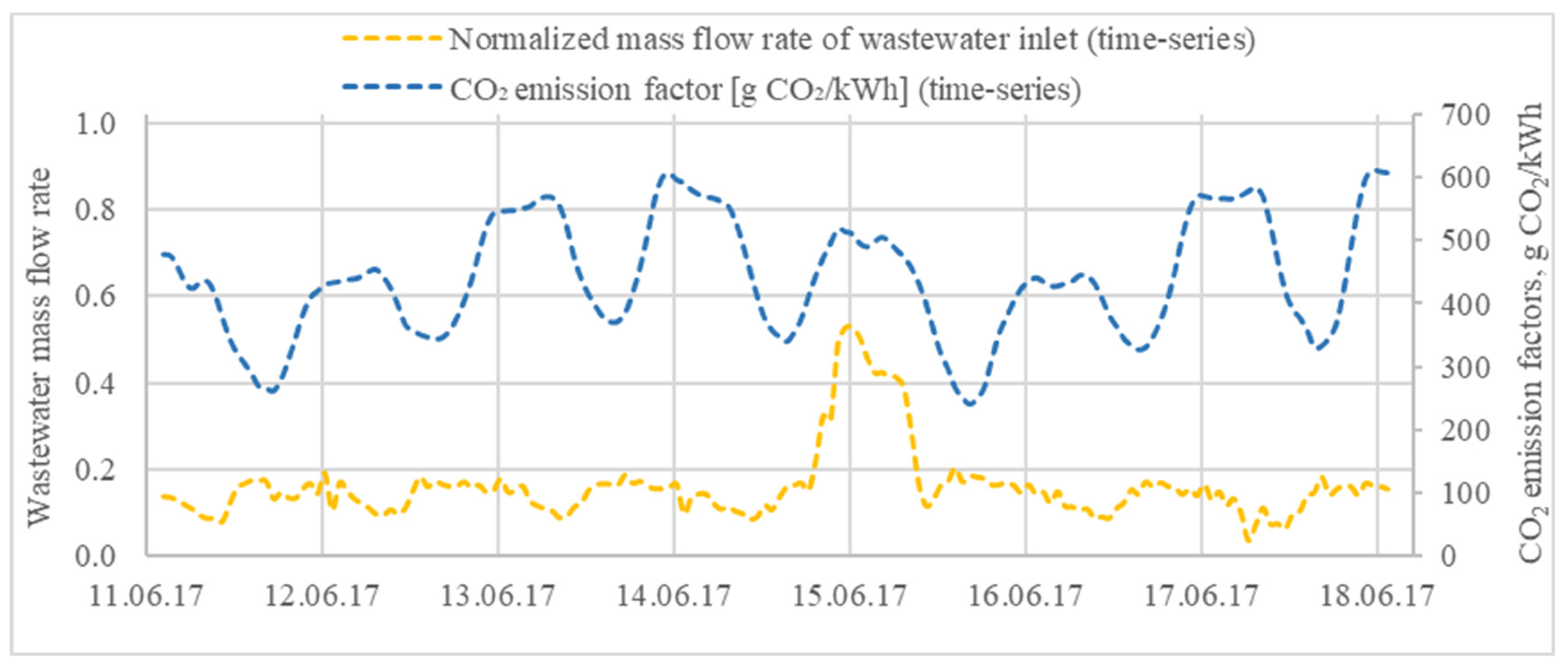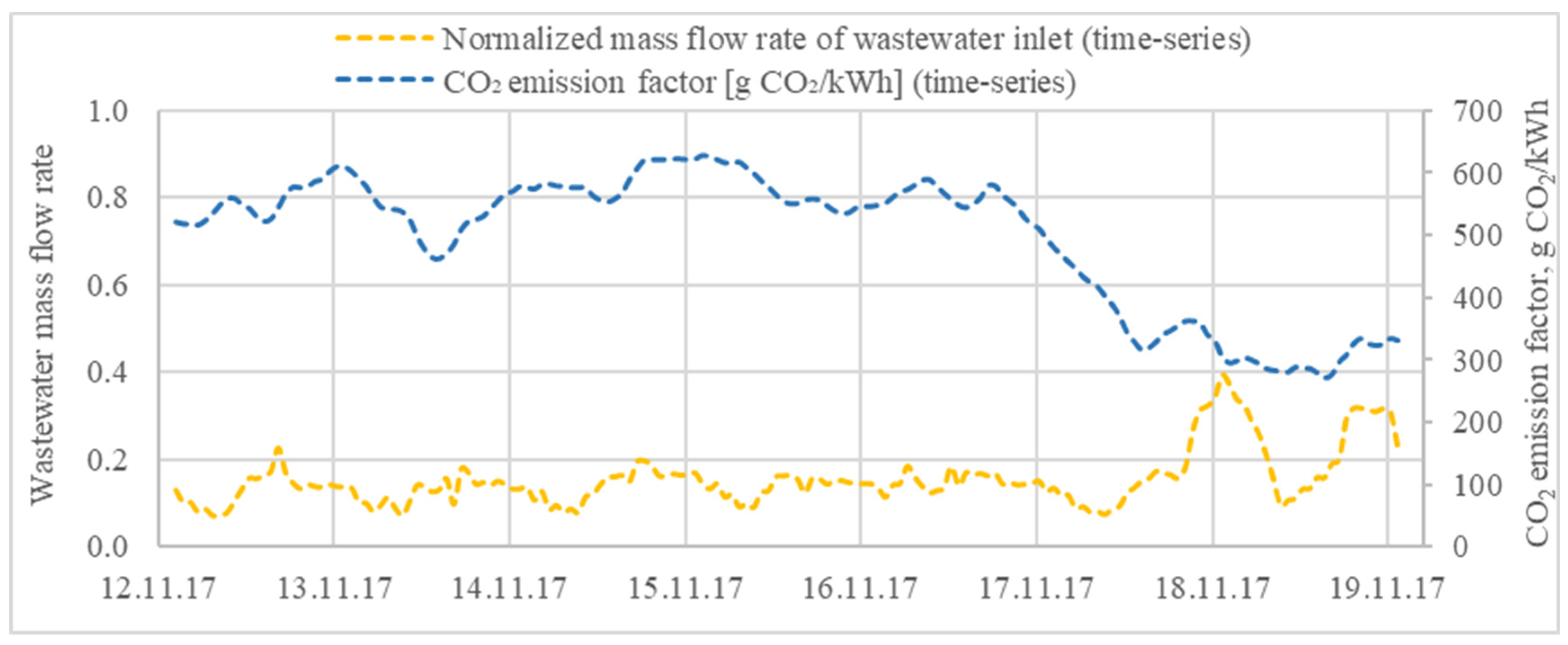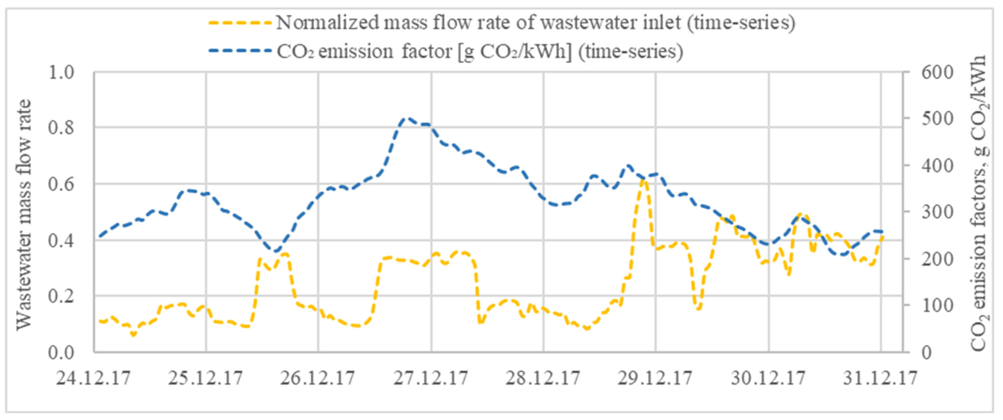However, when its share decreases, the share of the fossil-fuel-based electricity increases and so does the CO₂ emission factor of the grid. The values/trend of the CO₂ emission factor for each season are given in Figure A2, Figure A3, Figure A4 and Figure A5. By using this factor in the optimization model, a flexible behavior of the WWTP was aimed to be optimized depending on the fluctuating grid condition.

The user interface of the optimization model of the WWTP is given in Figure A1. It has 38 unit operations, 5897 equations, and 8796 variables.

2.4.2. Input Parameters

The input parameters of the WWTP model are described below:

• Within the MILP optimization approach, inlet and outlet temperatures and pressures of each unit must be defined initially as fixed values, as outlined in the previous subsection. They are used to calculate specific enthalpies, which become fixed coefficients in the linear equations of the model. When there is no major heating/cooling in the unit, the inlet temperatures of the units are set to be equal to the outlet temperatures. For heat exchangers, dryers, and digesters, setpoint values from the real plant were used. For these units, outlet temperatures are different from inlet temperatures during the optimization.
• Solid mass fraction of the sludge (w_TS) and organic mass fraction of the total solid within the sludge (w_oTS) were defined for each fuel stream in the related units as fixed set values. They were taken from the internal documents of EGK WWTP. Since the heating values of the sludge and the co-substrate and the composition of the fuel are both a function of w_TS and w_oTS, they are calculated in the related units before the optimization starts, which makes them a fixed value as well.
• The minimum and maximum mass flow rates and the maximum power consumption of the components, if any, were defined. The power consumption was calculated based on either a power demand factor (in kWh/L) or assuming a linear relationship between the inlet flow and the power consumption based on the maximum capacities.
• The ratio which was used to separate the main wastewater stream into two before entering the B-stage pools, the mass flow rates of the recycled B-sludge streams, the volumetric flow rate of the recycled sludge stream of the digester, and the maximum allowable limit for the fuel flow to the WIP were fixed in the model based on EGK data.
• A portion of the cleaned water is used to rinse the filters, while another portion is sent to the WWTP and the WIP for internal use. The yearly average mass flow rates of these streams and the corresponding power consumption of the related pumps in these streams were defined as fixed values for simplicity.
• Heat loss occurs in the dryers, so the efficiency of heat utilization was defined for this component.
• Water storage pool parameters such as the capacity (in mass) and the maximum loading and unloading mass flow rates of the storage were defined initially. The capacity is the maximum mass of the water that can be stored in the storage volume. The maximum loading and unloading rates depend on the related pumps.
• Parameters of the fuel storage tank are different from the water storage pool parameters, such as their capacities ($E_{storage}$) and maximum charging and discharging fuel rates (${\dot{e}}_{storage}$), which must be defined initially as energy and power units, respectively. The capacity of the storage tank is calculated by using the storage volume ($V_{storage}$), the fuel density ${(\rho }_{fuel}$), and the fuel’s heating value (${Hu}_{fuel}$) as given below [50]:

  $$E_{storage}=V_{storage}\ast {\rho }_{fuel}\ast {Hu}_{fuel}$$

  (1)
  The maximum charging and discharging rates depend on the related pump’s maximum volumetric flow rate (${\dot{V}}_{fuel}$), the fuel density, and the heating value of the fuel [50]:

  $${\dot{e}}_{storage}={\dot{V}}_{fuel}\ast {\rho }_{fuel}\ast {Hu}_{fuel}$$

  (2)

2.4.3. Input Variables

Hourly time series, defined for the whole year, were used in the model as independent input variables. They were based on real plant data from 2017 supplied by EGK. The inlet flow rates of the wastewater were recorded hourly. Since the co-substrate supply is only available as the total volume per month, an hourly feeding time series was created based on the monthly average. The properties of the co-substrate such as the composition, the heating value, etc. also differed for each month, so a time series was defined for each of them based on their monthly average values. Since the capacity and the charging and discharging rates of the fuel storage tanks must be defined in energy and power units, respectively, they also change based on the properties of the co-substrate. Therefore, a time series was defined for each of them in the co-substrate storage unit to ensure that the volume of the storage and the volumetric charging and discharging fuel rates were constant throughout the whole year. Finally, the minimum and the maximum filling levels were defined as constraints for all the storage components to ensure that the initial and the final filling levels would be the same due to the reasons given in Section 2.4.6. The CO₂ emission factors of the German electricity mix and the outside temperature values of Krefeld, which were obtained from Germany’s National Meteorological Service [51], were also used in the model as time series.

2.4.4. Optimization Variables

The hourly feeding mass flow rate of the co-substrate was optimized by utilizing the storage option to reduce the WWTP’s CO₂ emissions. The mass flow rates of other fuel and water streams were optimized as well, wherever a storage option was available and/or a part-load behavior or a shut-down of a unit was possible. As a result, the total mass flow rate of the wastewater into the A-stage pools was optimized. The main optimization variables used in the WWTP model are given in

Table 1. The optimization variables discussed in the results section.

1	Mass flow rate of the A-sludge into the mixers
2	Mass flow rate of the co-substrate into the digesters
3	Mass flow rate of the biogas into the WIP
4	Mass flow rate of the digested sludge into the centrifuges-2
5	Mass flow rate of the thick sludge into the dryers
6	Mass flow rate of the dried sludge into the WIP
7	Charging and discharging rates of the sludge storage tanks
8	Outlet mass flow rate of the process water treatment pool
9	Inlet and outlet mass flow rates of the excess water storage pool

. The filling levels of these storage units were calculated correspondingly. The hourly heat demand of the dryers, the heat exchangers, and the digesters and the power demand of the pumps, the compressors, the centrifuges, and the dryers result from the optimized operation. The upper and the lower boundary conditions of the optimization variables are the maximum and the minimum mass flow rates and/or power consumption of the units based on the available infrastructure of the Krefeld WWTP. The optimizer can operate the units within these limits based on the CO₂ emission factor of the grid to minimize the CO₂ emissions.

2.4.5. Optimization Period

Originally, the WWTP model was integrated to a WIP model and a district heating model of Krefeld. This integrated model, named the overall model, was decided to be run for 2017 and its total annual CO₂ emissions were aimed to be evaluated. Since only weekly optimization of the overall model with hourly discretization took 2.5–26 h to be completed, a representative week for each season was decided to be chosen based on statistical variables. Then, the overall model would be run only for these 4 weeks and the results would be used to project to a generalized annual result. For this purpose, the CO₂ emission factors were calculated on an hourly basis by using German electricity market data for 2017 [52]. Then, they were sorted by season. The variables describing the characteristic hourly gradient (as change in the CO₂ emission factor per hour) and variance were formed in each case. Using these variables and weighting factors, the most representative week for each season was determined (

Table 2. Representative weeks for each season of 2017.

Season	Date Interval
Spring	13–19 March 2017
Summer	12–18 June 2017
Autumn	13–19 November 2017
Winter	25–31 December 2017

). These four weeks were also used for the validation and the optimization of the WWTP model.

2.4.6. Initial Values and Endpoint Constraints

A general difficulty with storage units is how to set reasonable initial values for the filling level. An obvious choice would be setpoint values of the real plant. However, these values were never designed with the goal of flexible operation in mind. As the goal of this study is to assess the potential of flexible operation, an initial filling level of 50% was chosen because it offers the largest flexibility in both directions.

To keep the mass, energy, and emission balances consistent, it is also necessary to fix the final filling level to the same value as the initial value, 50%. Otherwise, emissions would be avoided in the optimized time interval but would occur at a later point in time and would not be accounted for. When optimizations were performed without this constraint, the storage units were always empty or full after the last time step, depending on its position with respect to a power-consuming unit. Therefore, minimum and maximum filling levels such as 49.99% and 50.01%, respectively, were defined as constraints for both initial and final filling levels of storage units at the first and the last time step of the optimization.

Note that the model is too complex to be run for an entire year (see previous subsection). The optimization was performed for one representative week per season and then projected to an entire year. This makes consistent balances even more important. When the final filling levels are equal to the initial ones, it is possible to combine the results for each week to form a feasible result for the entire year. The optimization of an entire year would have more degrees of freedom and might achieve an even higher emission savings potential, so the results of this study can be considered conservative.

Of course, the endpoint constraint can result in nonintuitive usage of the storage units in the last few hours of a week. This will be discussed in more detail in the results section.

2.5. Validation of the WWTP Model

To validate the WWTP model, it was firstly simulated for 1 time step by using the annual averages of the real-time plant data for w_TS, w_oTS, inlet flow rates of wastewater, and co-substrate. This model did not include any time series or storage units. So, there was no degree of freedom. Inlet and outlet mass flow rates of each unit were compared with the plant’s data during the validation, but only the outlet mass flow rates of the WWTP’s two end products, dried sludge and biogas, were chosen to be presented in this paper. The annual average of the dried sludge and the biogas production rates differed only by 1.1% and 1.7%, respectively.

Secondly, the WWTP model was decided to be run for one month that included the chosen week (

Table 3. The difference (absolute values) between the monthly average values of EGK WWTP data and the WWTP-OPT model for each season.

Season	Date Interval	Month for Validation	Dried Sludge Production Rate, %	Biogas Production Rate, %
Spring	13–19 March 2017	March	1.3	0.3
Summer	12–18 June 2017	June	1.3	0.5
Autumn	13–19 November 2017	November	1.7	0.8
Winter	25–31 December 2017	December	1.1	1.2

) because the dried sludge production data and the co-substrate supply to the plant were only available on a monthly basis. Therefore, the time series mentioned in Section 2.4.3 and the storage units were added to the WWTP model to convert it to an optimization model named WWTP-OPT. However, the monthly average of the optimization model for the dried sludge and the biogas production would be equal to the simulated results because their monthly average production rates would not change due to the same input of the wastewater and the co-substrate to the plant. The average values of the production rates of the dried sludge and the biogas were compared with the monthly average values of the EGK WWTP data for each season in Table 3. As a result, the validation of the WWTP-OPT model was found to be successful. The linearized equations in the model adequately represent reality.

3. Results and Discussion

The optimization results are given in this section. Then, the effects of two scenarios are discussed regarding reduction of the CO₂ emissions beyond the optimized level.

3.1. Analysis of the Main Optimization Results of the WWTP-OPT Model

Firstly, the driest and the wettest weeks of 2017 were determined. The driest week was 21–27 August 2017, whose average wastewater inlet was 39.5% less than the yearly average of 2017. On the other hand, 20–26 July 2017 was the week with the highest average of wastewater inlet which was 112.3% higher than the yearly average. The optimization model was run for these two weeks to test its limits. Both runs were completed successfully, which meant that the capacities of the components of the model were defined well enough to handle the extreme conditions.

Afterwards, the model was optimized for each representative week given in Table 2, but only a graph of one season per case is presented in this section since the model behavior is more or less the same for each season. Generally, the optimizer tries to move the operation of large consumers like dryers and centrifuges to periods with low CO₂ emission factors by using the various storage options in the plant. In this section, various sub-flowsheets with relevant storage options are discussed in detail in downstream order.

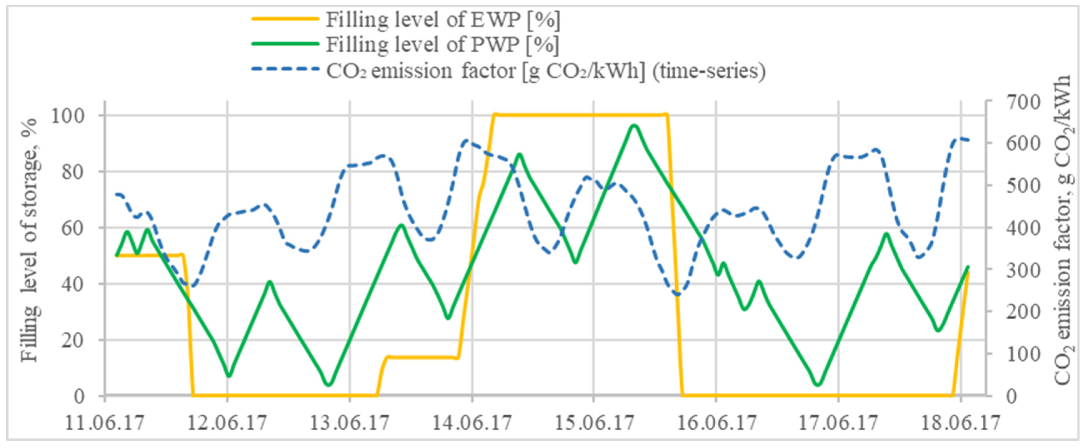
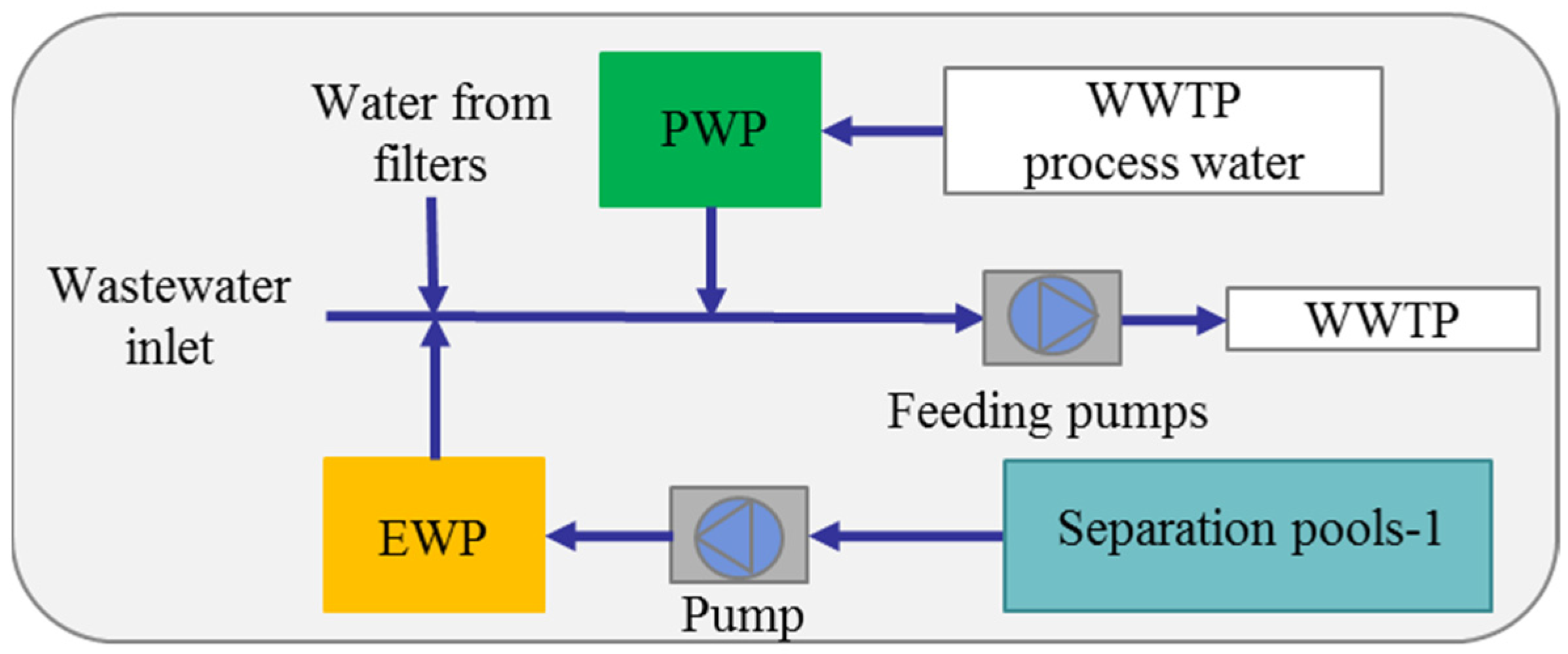
In normal operation, all the wastewater coming to the plant and the water used to clean the filters are sent to treatment by the inlet feeding pumps (Figure A6). However, internally produced wastewater streams from the centrifuges, the dryers etc. are collected in the PWP. Wastewater can also be stored in the EWP under extreme conditions such as heavy rain. Both pools discharge water to the inlet feeding pumps and their operations were optimized in the model to save CO₂ emissions. 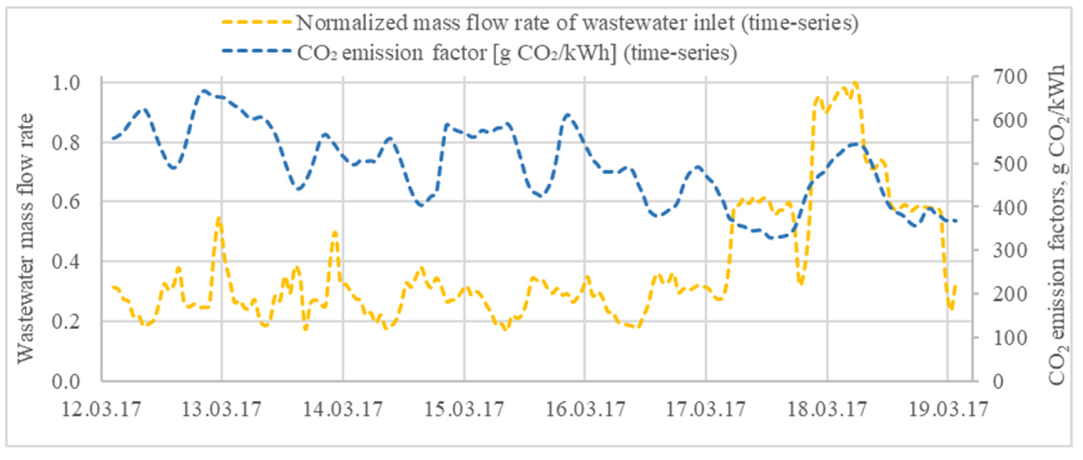Figure 3 shows the optimized operation for the summer week. Both pools are charged and discharged several times because the CO₂ emission factor changes continuously in a wider range of 242–612 g CO₂/kWh. Generally, they discharge water during lower ranges of the CO₂ emission factor, while they store water to decrease the WWTP’s load when the CO₂ emission factor is relatively higher. The operation of the PWP follows the CO₂ emission factor more closely since there is no power consumer such as a pump in its charging stream that would cause indirect CO₂ emission through the electricity usage. However, the EWP is charged/discharged less frequently because of its powerful inlet pump (Figure A6).

In the last few hours of the week, both storage filling levels return to 50% because of the endpoint constraint explained in Section 2.4. Higher final filling levels could have saved some more indirect emissions in this week. However, the optimizer cannot know if this is a reasonable strategy, as the following week could start with an even higher emission factor. In this case, low storage levels at the endpoint would be favorable for even higher savings in the following week. This conservative underestimation of the potential was expected (Section 2.4). Nevertheless, extensive use of flexibilities within the week can be observed because most weather-induced fluctuations in the energy system occur within one or a few days. This holds especially for the PWP, such that the behavior in the last few hours will have a minor effect on the overall result.

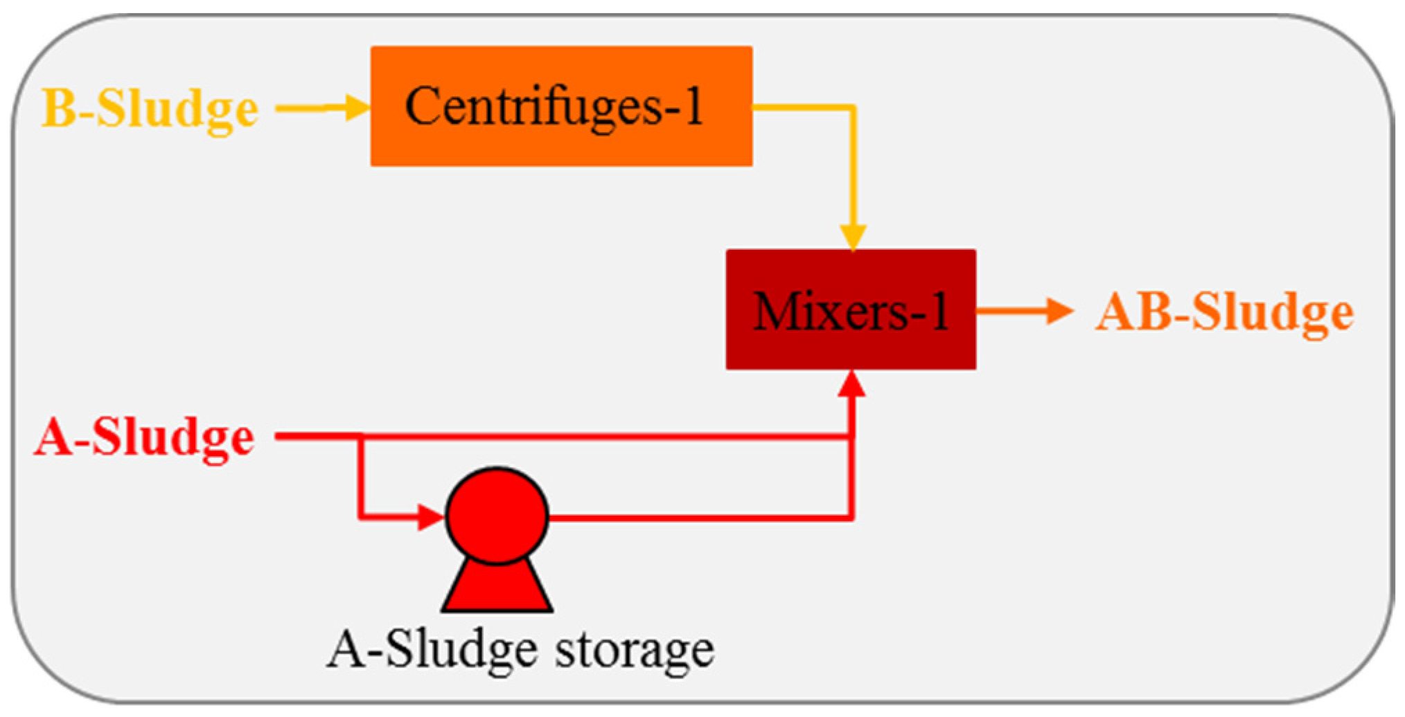
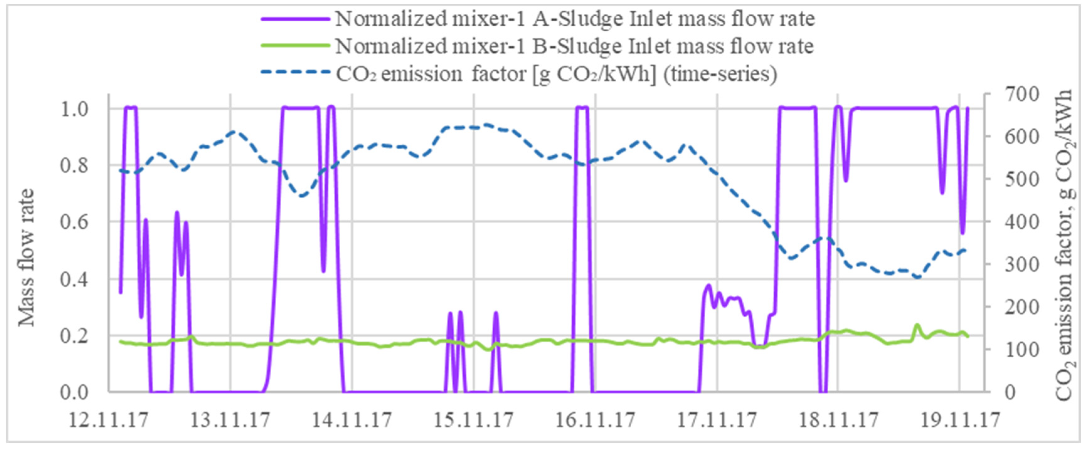
As seen from Figure A7, the A-sludge has a storage option before being sent to the sludge treatment part, while the B-sludge has no storage option and must be treated continuously as it is produced. In Figure 4, the effect of the storage option on the feeding of the A-sludge can be clearly seen for the autumn week. The optimizer sends the produced A-sludge from the storage to the sludge treatment only during the lower ranges of the CO₂ emission factor to prevent the operation of the following powerful components such as the centrifuges-2 and the dryers to save CO₂ emissions.

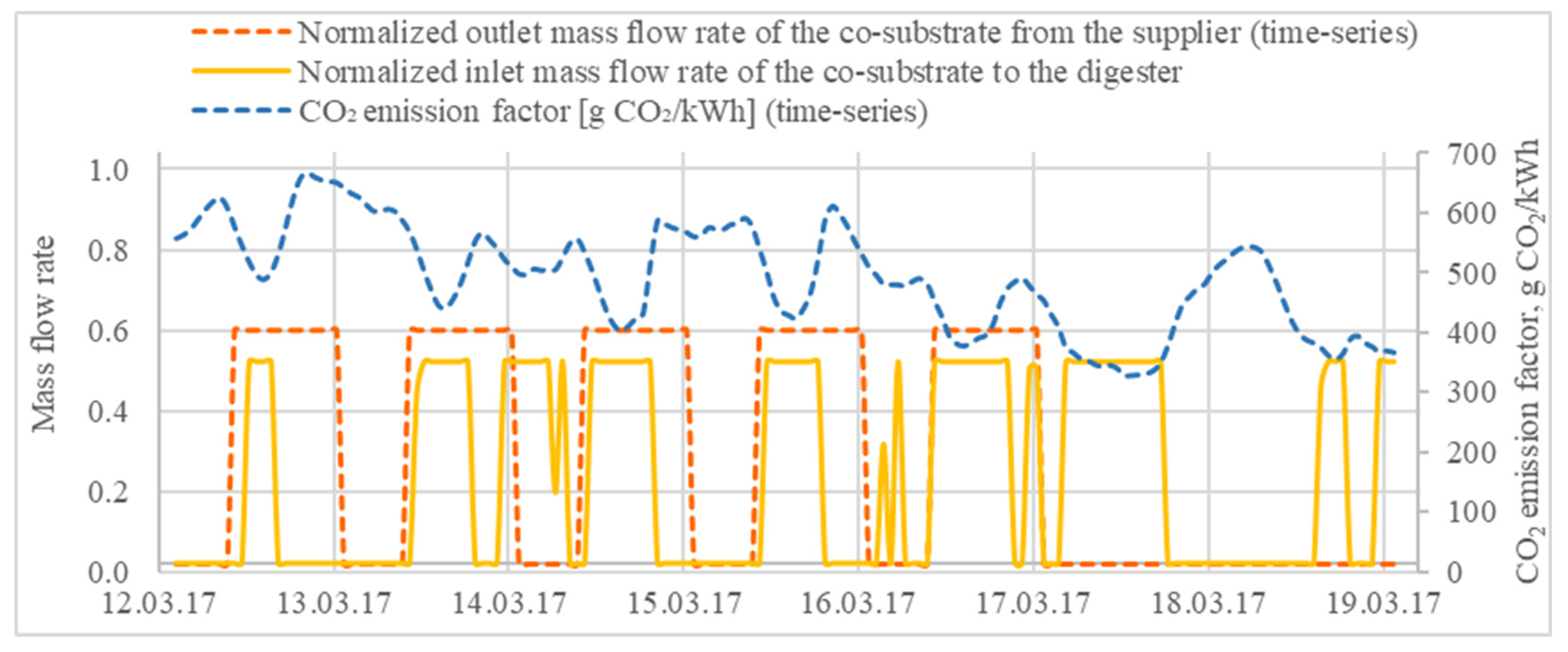
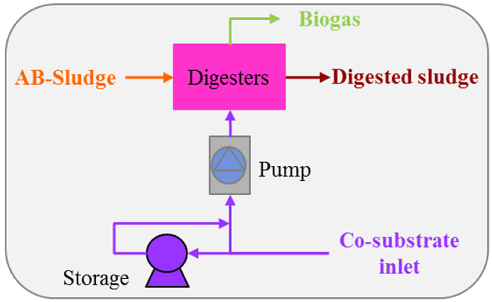
The incoming co-substrate to the Krefeld WWTP was described by an hourly time series throughout the whole year, but its feeding rate to the digesters can be optimized with the help of the co-substrate storage (Figure A8). The feeding rate is limited by the pump capacity. There is a continuous AB-sludge influent to the digesters in the WWTP as explained in Section 2.3, no. 4. The feeding of the co-substrate is realized during the low ranges of the CO₂ emission factor. While none is sent during high ranges to decrease the production of the digested sludge and the biogas, it would cause further power consumption and CO₂ emissions in the following components such as the centrifuges-2 and the dryers (Figure 5, spring week).

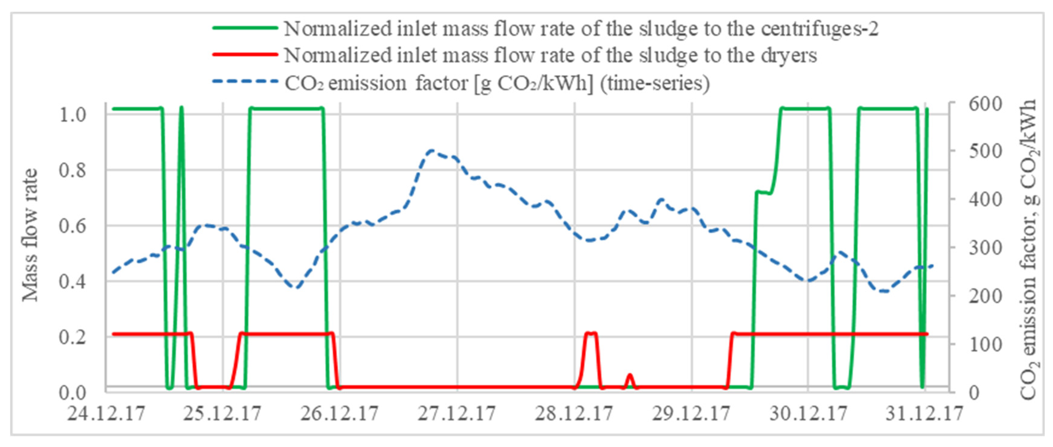
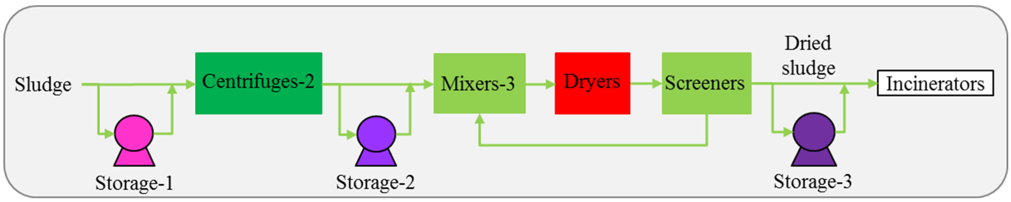
The sludge treatment part of the WWTP has two powerful components, the centrifuges-2 and the sludge dryers, and three storage options in between these components (Figure A9). The operation of the centrifuges-2 and the dryers can be optimized to lower the CO₂ emissions (Figure 6, winter week). At higher ranges of the CO₂ emission factor, the optimizer either shuts them down or reduces their capacities to decrease the power consumption and CO₂ emissions.

However, operational flexibility is mostly observed as the shut-down of the units. The optimizer might also operate the units at partial loads, there is no obstacle for this. If this is not carried out, the only reason is that this behavior would increase the CO₂ emissions. The sludge storage units are utilized for the flexible operation of the centrifuges-2 and the dryers. In the middle of the week, when CO₂ emission factors are the highest and the units are mostly shut down, the sludge is sent to the WIP from the storage-3. The storage-2 has a relatively small volume that can be emptied or filled completely in a short time, which puts a limit on the flexible operation of the units.

3.2. Estimated Saving of the CO₂ Emissions

To see the effect of the flexibility on the reduction of the CO₂ emissions, a so-called WWTP-REF model was developed based on the WWTP-OPT model because real hourly operation data from the Krefeld WWTP were not available throughout the whole of 2017 for comparison. Firstly, the time series of the wastewater inlet and the co-substrate supply were kept the same to represent the real plant behavior. Secondly, the average mass flow rates of the WWTP-OPT model’s main streams were as follows:

• A-sludge inlet to the mixer-1;
• Co-substrate inlet to the digesters;
• Sludge inlet to the centrifuges-2;
• Sludge inlet to the dryers;
• Dried sludge sent to the WIP;
• Biogas sent to the WIP.

It was decided to use in the WWTP-REF model to represent WWTP’s original operation. This is because WWTP’s priority is to treat the wastewater as it arrives at the plant and keep the operations of the processes continuous and in a steady state as much as possible.

These main streams were the only streams whose mass flow rates could be fixed with the help of the storage units. It was not possible to fix the mass flow rates of the other streams through the wastewater treatment pools, filters, and B-sludge process line due to the varying wastewater inlet and the lack of storage units in that plant section. The EWP and its feeding pump were removed since they were rarely used in the plant.

Normally, A-stage air compressors are operated on–off in the plant. However, the power consumption of these air compressors was assumed to be dependent on the properties of the inlet wastewater in the WWTP-OPT model. Therefore, the operation mode of the compressors was also modified to be on–off in the WWTP-REF model to represent the real plant.

The WWTP-REF model was run for four representative weeks. The CO₂ savings for each week were calculated by taking the difference of the total CO₂ emissions of the WWTP-REF and the WWTP-OPT models. These values were then multiplied by the number of the weeks in the corresponding season and summed up to estimate the annual CO₂ reduction potential. The reduction of the CO₂ emissions (%) are summarized for each season in

Table 4. Effects of the flexibility, the operation mode of the A-stage compressors, and alternative scenarios on the CO₂ emissions for each season and the entire year for 2017 (when compared with the WWTP-REF model).

Reduction of CO2 Emissions, %
Name of Model	WWTP-COMP	WWTP-OPT	WWTP-OPT-1			WWTP-OPT-2
Change in Model	Compressors’ Mode (Linear)	Compressors’ Mode (Linear) + Flexibility	Compressors’ Mode + Flexibility + a Virtual B-Sludge Storage Unit			Compressors’ Mode + Flexibility + Position of EWP
			3600 m3	7200 m3	10,800 m3
Summer	3.3	5.9	7.7	7.8	7.8	9.1
Autumn	3.0	5.1	6.6	7.2	7.7	5.9
Winter	1.9	4.1	5.8	6.3	6.4	4.8
Spring	2.2	4.1	5.6	5.8	5.9	5.0
Year	2.6	4.8	6.4	6.7	6.9	6.2

. The calculated annual reduction is also given in the last row. When compared, the WWTP-OPT model causes a 4.8% reduction in annual CO₂ emissions due to flexibility. As mentioned in Section 2.2, this 4.8% reduction in the CO₂ emissions of the WWTP-OPT model corresponds only to 29.5% of the power consumption of the WWTP. It would be possible to reduce the CO₂ emissions much further by increasing the share of the power consumers in the flexible operation.

To see the effect of the operation mode of the A-stage compressors, only their operation mode was changed to be linear in the WWTP-REF model and the updated model is named WWTP-COMP. The WWTP-COMP model was run for each representative week and the corresponding CO₂ savings were calculated for each season and the year (Table 4). When compared, the 2.6% decrease in the annual CO₂ emissions results only from the change in the operation mode of the A-stage compressors, whose share is 8.3% in the power consumption of the WWTP. This gives a reasonable hint about the impact of the air compressors on the reduction of the CO₂ emissions, assuming they are operated flexibly, including shut-down, and based on the CO₂ emission factor of the grid.

3.3. Alternative Scenarios to Decrease the CO₂ Emissions

Thirteen alternative scenarios were studied to observe whether the CO₂ emissions of the WWTP-OPT model could be further decreased beyond the optimized case. In the alternative scenarios, either virtual storage units were added or the capacities of the present storage units and/or aggregates were increased, or the position of a storage was changed. Two of them with the highest impact on the reduction of the CO₂ emissions are presented in this paper.

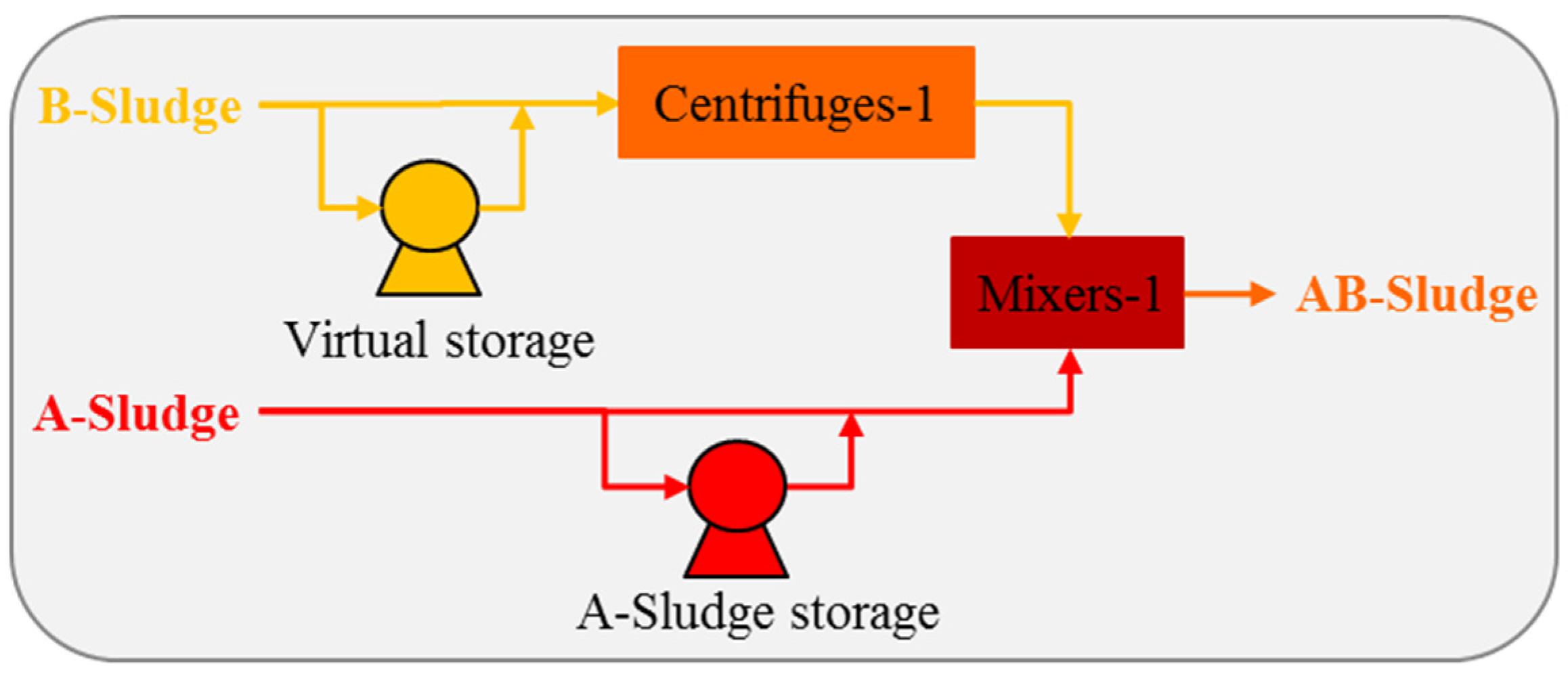
3.3.1. Scenario 1: Addition of a Virtual B-Sludge Storage

As mentioned in Section 3.1 and seen in Figure A7, the B-sludge has no storage option, so it has to be directly sent to the sludge treatment as it is produced regardless of how high the CO₂ emission factor of the grid is. 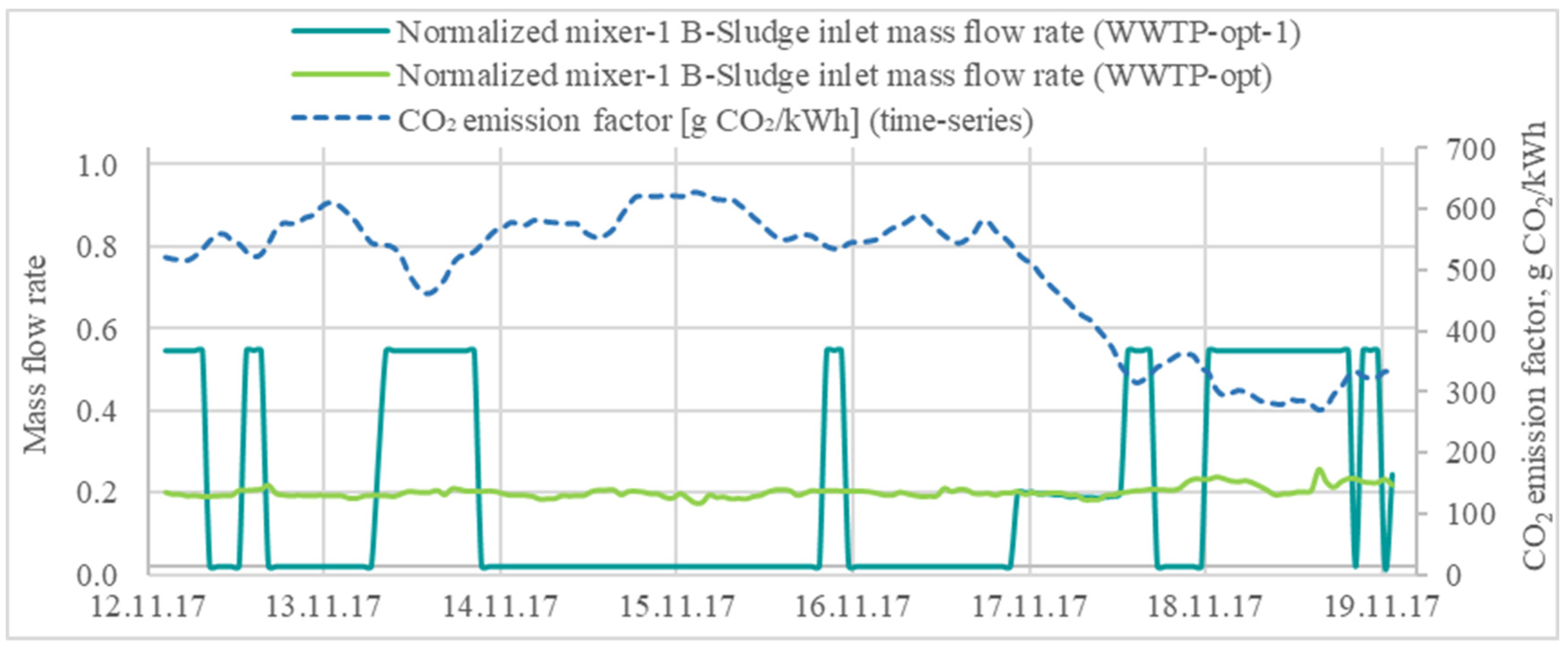Therefore, a virtual B-sludge storage unit was added between the separation pools-2 and the centrifuges-1 to increase the WWTP-OPT model’s flexibility and decrease its CO₂ emissions (Figure A10). This alternative model is called WWTP-OPT-1. The addition of the storage unit affected the operation of the centrifuges-1. These two models can be compared in Figure 7 for the autumn week. While the centrifuges-1 operate continuously in the WWTP-OPT model, they can be operated flexibly depending on the CO₂ emission factor in the WWTP-OPT-1 model with the help of the virtual storage unit. The centrifuges-1 operate at their highest capacities during the low ranges of the CO₂ emission factor and then they are shut down or partially operated at high ranges of the CO₂ emission factor. By utilizing a virtual B-sludge storage unit, the CO₂ emissions are reduced by 6.4–6.9% yearly, depending on the storage volume, when compared to the WWTP-REF model (Table 4).

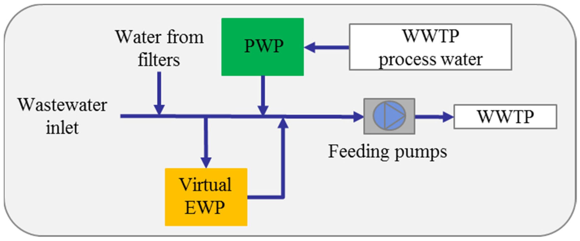
3.3.2. Scenario 2: Positioning the EWP at the WWTP’s Inlet

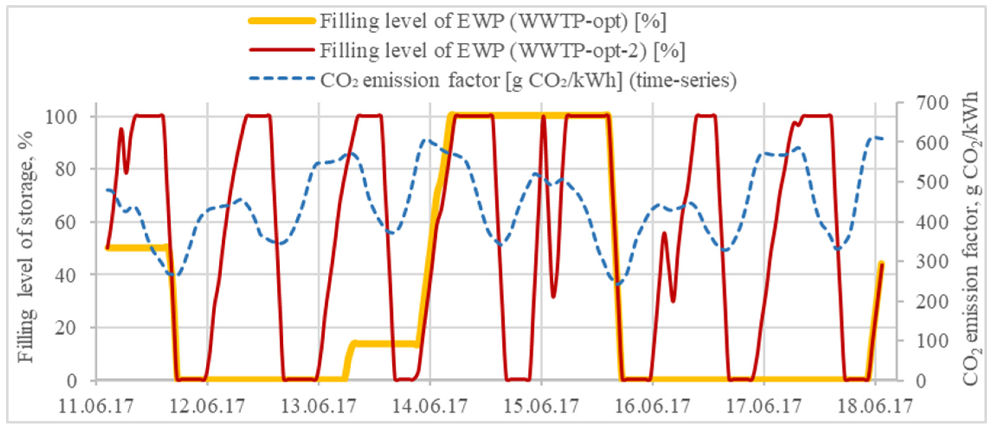
In this alternative scenario, the EWP was assumed to be placed at the WWTP’s wastewater inlet before the main feeding pumps (Figure A11), so that the wastewater could be directly stored before being sent to treatment. The feeding pump of the EWP was also removed by assuming that the EWP was positioned on the same level of the wastewater inlet. This alternative model is called WWTP-OPT-2. The behavior of the virtual EWP in the WWTP-OPT-2 model (Figure 8) is basically like the behavior of the EWP in the WWTP-OPT model (Figure 3) in following the CO₂ emission factor. The EWP is loaded at high values of the CO₂ emission factor and unloaded at low values. 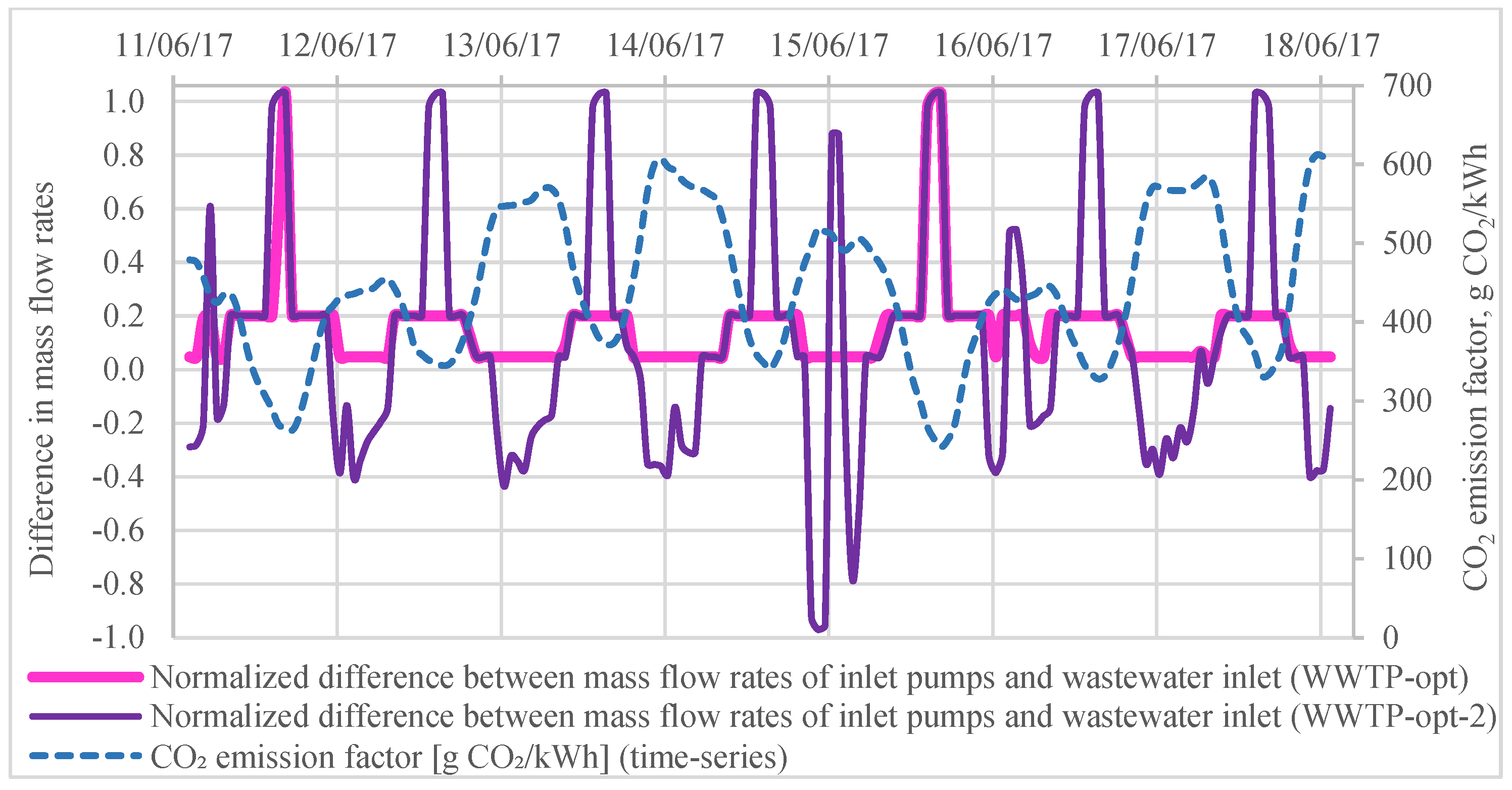However, in the WWTP-OPT-2 model, the EWP is more flexible and used frequently due to its position and lack of a power consumer at its inlet that would cause CO₂ emissions when operated. The difference between the mass flow rates of the feeding pumps and the wastewater inlet to the plant is compared (Figure 9, summer week), and negative differences are observed during higher ranges of the CO₂ emission factor. This means that less wastewater is sent to the plant to decrease the load and the CO₂ emissions, which was not possible in the WWTP-OPT model. When compared to the WWTP-REF model, the annual CO₂ reduction of the WWTP-OPT-2 model is estimated to be 6.2% (Table 4). This adaptation causes a load shifting through the whole plant based on the CO₂ emission factor of the grid.

4. Conclusions

In this case study of the Krefeld WWTP, various DSM options were considered, and their potential to save CO₂ emissions was assessed. An MILP optimization model was built, validated, and run for four weeks, each of which represents a season. The target function was to minimize the WWTP’s CO₂ emissions, which are indirect emissions calculated by the hourly CO₂ emission factor of the electricity grid. Large power consumers of the Krefeld WWTP such as centrifuges and dryers are either shut down or operated at partial loads with the utilization of storage units during the higher ranges of the CO₂ emission factor. When the CO₂ emission factor of the grid decreases, these units are either started up or their capacities are increased. Flexible feedings of the wastewater and the co-substrate are also possible due to the available storage units. As a result, annual indirect CO₂ emissions of the Krefeld WWTP decrease by 4.8% due to the flexible operation of the units, whose share in total power consumption is 29.5%. Increasing the share of the units in the flexible operation would definitely decrease the CO₂ emissions further.

It was observed that the flexibility of the WWTP is limited depending on its storage capacities. Therefore, it is possible to enhance the flexibility of the WWTP and its CO₂ savings potential by either increasing the capacities of the available storage units or adding new storage units. It is shown in the alternative scenarios (Section 3.3) that an addition of a B-sludge storage would reduce the indirect CO₂ emissions by 6.9%.

In this case study, the load-shifting potential of the Krefeld WWTP within demand side management was proved by an optimization model. This model is promising to be applied to other WWTPs by adjusting the specifications of the units, the operating conditions, and the constraints, but it still needs to be validated in real operation.