Improvement and Evaluation of CLM5 Application in the Songhua River Basin Based on CaMa-Flood

Abstract

This paper optimized the hydrological postprocessing of CLM5 using CaMa-Flood, combining multi-source meteorological forcing datasets and a dynamically changing surface dataset containing 16 PFTs (plant functional types) to simulate the high-resolution runoff process in the SRB from 1996 to 2014, specifically by integrating discharge with flooded area. Additionally, we evaluated the spatiotemporal variations of precipitation data from meteorological forcing datasets and discharge to validate the accuracy of model improvements. Both the discharge and the flooded area simulated by the coupled model exhibit pronounced seasonality, accurately capturing the discharge increase during the warm season and the river recession process in the cold season, along with corresponding changes in the flooded area. This highlights the model’s capability for hydrological process monitoring. The simulated discharge shows a high correlation coefficient (0.65–0.80) with the observed discharge in the SRB, reaching a significance level of 0.01, and the Nash–Sutcliffe efficiency ranges from 0.66 to 0.78. Leveraging the offline coupling of CLM and CaMa-Flood, we present a method with a robust physical mechanism for monitoring and providing a more intuitive representation of hydrological events in the SRB.

1. Introduction

In recent years, in most parts of the globe, storm runoff extremes have systematically approached or exceeded historical precipitation extremes [1], accompanied by large spatial scales and variability on decadal timescales [2], and storm runoff extremes have increased at an approximate Clausius–Clapeyron rate [3]. China has experienced significant warming in recent decades and has already experienced some devastating climate extremes. For example, the Great Flood of 1998 inundated 24 × 10⁴ km² of land, destroying 5 million houses, including those in the Yangtze River basin and Songhua River Basin (SRB), and causing more than USD 20 billion in economic losses [4], while studies in the Tibetan Plateau have shown that the risk of flooding is projected to increase with warming temperatures [5]. Northeastern China, where the SRB is located, is one of the most important agricultural regions in the world [6] and home to China’s largest plain [4]. Due to socioeconomic development and intensification of agricultural production in the SRB, the demand for water resources has increased rapidly. The SRB is also an area prone to extreme flooding. Many hydraulic structures have been constructed in the SRB, and these infrastructures can prevent flooding during the rainy season and alleviate water scarcity during the dry season [7]. Studying the spatial and temporal variability of runoff throughout the SRB is important for water resource management and for maintaining sustainable socioeconomic and agricultural production.

Discharge is one of the most comprehensive indicators of the overall impact of various factors in basin-scale hydrology [8,9,10], and accurately modeling discharge is key to understanding the water cycle, water resource management, and climate change. There are various research methods to simulate discharge, such as using the water balance equation combined with precipitation, evapotranspiration, and terrestrial water storage anomaly (TWSA) measured by GRACE Follow-On (GRAFO) to derive the production and sinking process; this method has been validated in the Yangtze River Basin, but the timeliness of the monthly GRAFO for TWSA monitoring is lacking [11,12]. Land surface models (LSMs) driven by meteorological forcing data can simulate discharge at multiple time scales (from monthly to interannual) [13], and LSMs require more meteorologically forcing data than traditional distributed hydrologic models (DHMs), such as precipitation, solar radiation, near-surface air pressure, near-surface wind speed, near-surface air moisture content, and near-surface air temperature data. Weather stations can also measure water fluxes, but the data obtained are at the point scale only, and the scarcity of meteorological stations in developing countries causes the need to seek other more comprehensive and reliable meteorological forcing data to drive models [14]. If the meteorological forcing data are inaccurate, even if the model can handle high-resolution data and has a strong physical mechanism, it will not enhance the accuracy of the model simulation results [15]. Therefore, reliable and accurate meteorological forcing data are essential for LSMs.

The Community Land Model (CLM) is a common and widely used LSM and the land component of the Community Earth System Model 2 (CESM2) [16,17]. We used CLM5, which has been updated from the development of CLM4 [17] and CLM4.5 [18], but the improvements in CLM5 still do not simulate changes in flooded areas on time scales, and most of the previous work on flood characterization has been conducted using runoff data rather than flooded areas [19]. The catchment-based macroscale floodplain model (CaMa-Flood) is a global river hydrodynamic model that can perform high-precision simulations of confluence processes and flooded areas in large basins and has been validated in the Amazon Basin and the Yangtze River Basin [12,20]. In this study, we coupled the model with CLM5 to compensate for the shortcomings of CLM5 in runoff simulation.

The main objective of this study is to improve the hydrological postprocessing of the CLM utilizing CaMa-Flood, and on this basis, we provide a method with a strong physical mechanism for monitoring and presenting a more intuitive representation of hydrological events in the SRB to better understand floods from the perspective of discharge volume combined with flooded area. We enhanced the runoff processing after the land surface process simulation in CLM5 and first selected three sets of meteorologically forcing datasets, namely, CMFD (China Meteorological Forcing Dataset), GSWP3v1 (Global Soil Wetness Project dataset) and CRUv7 (Climatic Research Unit-NCEP forcing data), combined with a high-resolution subsurface dataset of the SRB to simulate the flooding process and obtain high-precision streamflow-producing data. These were then input into the CaMa-Flood to simulate the confluence process to investigate the runoff and flooded area changes. In addition, three representative stations in the SRB, namely, Harbin, Jiamusi and Tonghe, were selected for validation and evaluation. Finally, we present the simulation results for discharge and flooded area obtained from different meteorological forcing dataset-coupled models with simultaneous power downscaling.

2. Materials and Methods

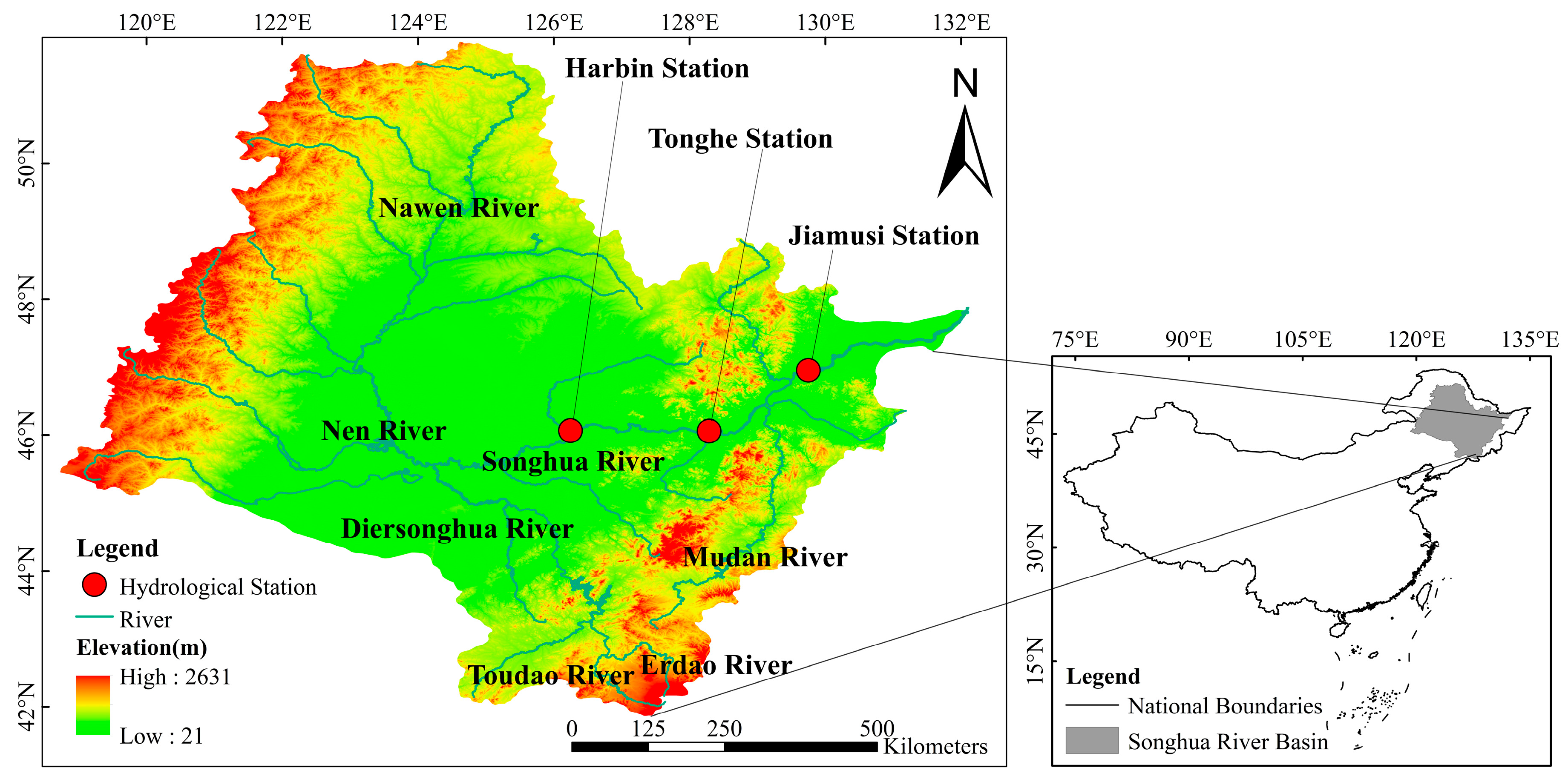
2.1. Study Area

The SRB is in northeastern China, spanning an elevation from 50 to 2700 m above sea level, with a longitude of 119°52′–132°31′ E and a latitude of 41°42′–51°48′ N. Covering an area of approximately 5.568 × 10⁵ km², the basin is characterized by mountainous terrain (61%) and plains (24%) [21,22,23]. Influenced by the high-latitude subpolar westerly winds and the mid-latitude monsoon climate, part of the SRB experiences subfreezing conditions, characterized by cold and lengthy winters and rainy summers. Precipitation varies across regions and seasons. Mountainous areas receive more rainfall than plains. Annual precipitation ranges from 350 to 1000 mm, with a long-term average below 500 mm. Of the yearly precipitation, 70% occurs between July and September. The average temperature in the region ranges from about 3 °C to 5 °C [24]. Due to its high topography in the northwest and southeast, poor drainage in the central area, and the impact of concentrated summer precipitation, the SRB has experienced severe flooding in recent years [25]. Flood occurrences are common in the SRB; however, there is a paucity of robust physical mechanism models for conducting high-resolution runoff process simulations. To enhance flood prevention, reduce economic losses in vulnerable areas, and optimize basin management, a high-resolution discharge simulation study was conducted. This study aimed to reflect the flooding process visually and precisely, facilitating better monitoring and early warning of floods based on discharge volume and flooded area [26]. Given that floods mainly occur in the middle and lower reaches of the basin, Harbin Station, Tonghe Station, and Jiamusi Station were selected for detailed analysis (Figure 1). These three hydrological stations provided daily flow observation data from 1996 to 2014.

2.2. Data

In this study, temporal resampling was performed to process its temporal resolution to 6 hourly. Three meteorological forcing datasets were used in this study: CMFD, GSWP3 v1, and CRUv7 (refer to

Table 1. General information of the meteorological forcing datasets. “Reanalysis” and “Observations” are corresponding datasets used in producing the atmospheric forcing. A detailed description can be found in Section 2.2.

Datasets	Resolution		Period	Reanalysis	Observations
	Temporal	Spatial
CMFD	6-hourly	0.1° × 0.1°	1979–2018	Princeton, CMA	TRMM, GEWEX-SRB, GLDAS
GSWP3 v1	6-hourly	0.5° × 0.5°	1901–2014	20CR	CRU TS v3.21, GPCCv7, SRB
CRU v7	6-hourly	0.5° × 0.5°	1901–2016	NCEP	CRU TS3.2

SRB stands for surface radiation budget.

for details). CMFD is based on internationally available TRMM precipitation data, GEWEX-SRB radiometric data, GLDAS data, and Princeton reanalysis data, combined with the CMA (China Meteorological Administration meteorological observational data), which now covers the period 1979–2018, with a temporal resolution of 3 hourly and a horizontal spatial resolution of 0.1° × 0.1° [27]. GSWP3 is the second version of the reanalysis dataset based on the NCEP model conducted in the 20th century. The raw data are dynamically downscaled by the spectral light-push data assimilation technique using the global spectral model. In addition, GSWP3 is bias-corrected for temperature, precipitation, longwave radiation, and shortwave radiation using the CRU TS v3.21, GPCC v7, and SRB (surface radiation budget) datasets, respectively [28]. GSWP3 v1, used in this, paper has a 6 hourly temporal resolution and a horizontal spatial resolution of 0.5° × 0.5°, with a coverage of the period 1901–2014 [29]. CRUv7 [30] is a 6 hourly, 0.5° × 0.5° resolution, globally forced product that combines two existing datasets: CRU TS3.2 and NCEP reanalysis. CRU TS3.2 provides 0.5° × 0.5° resolution monthly data covering 1901–2002, and the NCEP reanalysis provides 6 hourly data at 2.5° × 2.5° resolution covering 1948–2016. In this paper, we used version 7 of its data, which cover the period 1901–2016 and meet the needs of the study. Near-surface barometric pressure, specific humidity, air temperature, wind speed, precipitation, longwave radiation, and shortwave radiation from the dataset were used to force CLM5.

Soil data sources for CLM5 are more complex, with soil thickness data based on ORNL (Oak Ridge National Laboratory) [31] and land cover data from the USGS (U.S. Geological Survey) based on satellite data inversion of the GLCC dataset. Soil texture data were obtained from IGB (The International Geosphere–Biosphere Program) [32]. Soil color determines dry and saturated soil albedo, soil color data were obtained from MODIS, and LAI data were processed from the MODIS LAI dataset based on a range of properties of plant functional types (PFTs) obtained by mapping MODIS LAI monthly average data to different PFTs for each 0.05° grid [33]. LUH2 (Land-Use Harmonization²) provided historical and future scenario land use data from 850 to 2100 at 0.25° resolution. The LUH2 data were derived from the 850–2014 History Database of the Global Environment (HYDE version 3.2) and the Integrated Assessment Modeling Team (IAMT) for multiple alternative future scenarios from 2015–2100 [34]. Based on the above data, this study used the CLM land use data tool to generate a surface dataset and a dynamic land use dataset for the SRB at 0.1° resolution from 1996 to 2014 [35]. CaMa-Flood used MERIT Hydro, a global raster hydrographic map with 3 arc seconds resolution, elevation from MERIT DEM, and water body data based on G1 WBM (Global Surface Water Occurrence and OpenStreetMap) [36].

2.3. Hydrological Processes in CLM5

New to the hydrology section of CLM5 are the dry surface layers (DSLs) for representing evapotranspiration processes at the surface, spatially variable soil depths (0.4 to 8.5 m), vertical soil stratification (20 soil layers + 5 bedrock layers), adaptive time-step solving of the Richard equation, and the elimination of unconfined aquifers, with no flux lower boundary conditions. In the river simulation section, the River Transport Model (RTM) used in CLM 4.5 was replaced in CLM 5 by the Model for Scale Adaptive River Transport (MOSART) [37]. The main difference between RTM and MOSART is the way the river flow is calculated. RTM uses a simple linear reservoir approach where the flow transferred from a grid cell upstream of the RTM to an adjacent grid cell downstream of the RTM depends only on the amount of river storage in the upstream grid cell, the average distance between the grid cells, and a globally constant effective streamflow rate such that the RTM only simulates discharge (m³/s). In MOSART, river flow is calculated explicitly by the physically based kinematic wave method, a common approach in hydrology based on the mass and momentum equations, and in combination with detailed information on the hydrography of the simulation area (i.e., parameters describing river and tributary widths, depths, average slopes, roughness coefficients, and lengths of the main river). MOSART also simulates the flow velocity of the main river channel over time (m/s) and water depth, as well as subgrid surface water flow in hillslopes and tributaries [38].

CLM5 parameterized canopy interception, net precipitation, canopy dripping, snowpack and melt, water transport between snowpack layers, infiltration, evapotranspiration, surface runoff, subsurface drainage, redistribution within the soil column, and groundwater runoff and recharge to simulate changes in canopy water ΔW_can,liq, canopy snow water ΔW_can,sno, surface water ΔW_sfc, snow water ΔW_sno, soil water ΔW_liq,i, and soil ice ΔW_ice,i, as well as changes in water in the unconfined aquifer (all in mm H₂O).

The total water balance equation in this system is as follows [18]:

$$\begin{array}{c}\Delta W_{\mathit{can},\mathit{liq}}+\Delta W_{\mathit{can},\mathit{sno}}+\Delta W_{sfc}+\Delta W_{\mathit{sno} }+\sum _{i=1}^{N_{\mathrm{levsoi}}}\left(\mathsf{\Delta }{w}_{\mathrm{liq},i}+\mathsf{\Delta }{w}_{ice,i}\right)+\Delta W_a\\ =\\ \left(q_{\mathrm{rain}}+q_{sno}-E_v-E_g-q_{\mathrm{over}}-q_{h2osfc}-q_{drai}-q_{rgwl}-q_{snwcp,ice}\right)\Delta t\end{array},$$

(1)

where q_rain is liquid precipitation, q_sno is solid precipitation, E_v is evapotranspiration from vegetation, E_g is evapotranspiration from soil, q_over is surface runoff, q_h2osfc is surface water storage runoff, q_drai is subsurface runoff, q_rgwl and q_snwcp,ice are solid and liquid runoff from snow originating in glaciers, lakes, and other surface types, N_levsoi denotes the number of soil column layers in CLM5 (the hydrologic section accounts for the 1 − N_levsoi layer; (N_levsoi + 1) − N_levgrnd is not currently accounted for in the hydrologic component of the calculation), and Δt is the time step.

The water input at the surface of the grid cell is the sum of precipitation and snowmelt reaching the ground q_liq,0, and then the water flux is redistributed to surface runoff, terrestrial water storage, and infiltration into the soil. TOPMODEL implements a runoff parameterization, and the key concept in the model is the saturated area fraction, f_sat, which is determined by the grid cell’s topographic characteristics and soil moisture content. The saturated area directly affected the surface runoff q_over, according to the typical hillslope flow production process given by Dunn in 1975, with the following equation [18]:

$$q_{\mathit{over}}=f_{\mathit{sat}}·q_{liq,0}.$$

(2)

The relationship between the saturated area fraction and soil moisture content is as follows [18]:

$$f_{sat}=f_{max}\exp \left(-0.5f_{over}{z}_{\nabla }\right),$$

(3)

where f_max is the potential or maximum value of f_sat, f_over is the attenuation factor (m⁻¹), and z_▽ is the depth to the water table (m). z_▽ is determined by finding the first soil layer above the bedrock depth in which the volumetric water content drops below a specified threshold (the default threshold is set to 0.9). The maximum saturation fraction f_max is defined as the value of the discrete cumulative distribution function (CDF) of the topographic index when the average water table depth of the grid cell is zero. Thus, f_max is the percentage of pixels in a grid cell with a topographic index greater than or equal to the average topographic index of the grid cell and is calculated explicitly at each grid cell at the model-run resolution based on the CDF. An attenuation factor of 0.5 m⁻¹ was determined for the global simulation through sensitivity analysis and comparison with observed runoff [39,40,41].

2.4. CaMa-Flood

To compensate for the shortcomings of CLM5 for land surface process simulation, which can only obtain flow production data (unit: mm), and MOSART for flood simulation, CLM5 was coupled with CaMa-Flood, and the runoff data output from CLM5 was used to drive CaMa-Flood v4.1. The flowchart of the offline coupling model is shown in Figure 2. CaMa-Flood is a distributed global river network confluence model that is mainly used to simulate continental-scale rivers [20].

Based on the local inertia equation, CaMa-Flood calculates the river flow from each unit catchment to the unit catchment downstream by neglecting the second term of the 1-D St. Venant momentum equation Q (m³/s):

$$\frac{\partial Q}{\partial t}+\frac{\partial }{\partial x}\left[\frac{Q^2}{A}\right]+\frac{gA\partial \left(h+z\right)}{\partial x}+\frac{g{n}^2{Q}^2}{R^{4/3}A}=0.$$

(4)

Moreover, to extract subgrid topographic parameters from the ground elevation data (MERIT DEM) and river network map (MERIT Hydro) of the SRB with 3 arc seconds resolution, the flexible location of waterways (FLOW) method was also used in CaMa-Flood to extract the river channel length (L), river channel width (W), and bank height (B); and the channel storage S_r, floodplain storage S_f, channel water depth D_r, floodplain water depth D_f, and inundation area A_f were calculated from the total storage S (where D_f was obtained by the CDF representing the function between water level and inundation area of a unit’s catchment, D_f = D(A_f)) [42,43,44].

2.5. Methods

The study is divided into two parts: The objective of the first part is to assess the suitability of precipitation data from various observational satellites and reanalysis in a meteorological forcing dataset, then to obtain high-resolution runoff data for the period 1996–2014 by integrating land surface process simulations with a dynamic surface dataset at 0.1° resolution. In the second part, three sets of runoff datasets obtained from the simulation were used to force the hydrological model to obtain the SRB resolution 1′ × 1′ discharge and flooded area datasets. Finally, the accuracy and applicability of the runoff simulation results were evaluated to determine whether the coupled model was applicable in the SRB.

The comparison of precipitation data from stations and meteorological forcing datasets used two statistical metrics: the correlation coefficient (CC) and root mean squared error (RMSE). Coefficients of variation (CV), correlation coefficient (CC), relative bias (RB), and Nash efficiency coefficients (NSE) were used for the coupled-model runoff simulation results because they are commonly used in runoff uncertainty assessments [8,45,46]. The expressions and specific descriptions of each evaluation metric are shown in

Table 2. Evaluation index expressions, ranges, ideal values, and description in the study.

Index and Expression	Range and Ideal Value	Description
$(1) CC=\frac{{\sum }_{i=1}^n(Q_{ti}-\stackrel{\leftharpoonup }{Q_t})·(Q_{pi}-\stackrel{\leftharpoonup }{Q_p})}{\sqrt{{\sum }_{i=1}^n{(Q_{ti}-\stackrel{\leftharpoonup }{Q_l})}^2·{\sum }_{i=1}^n{(Q_{pi}-\stackrel{\leftharpoonup }{Q_p})}^2}}$	[−1, 1], 1	Qti and Qpi denote the observed and unobserved values at time point i, respectively; Qt and Qp represent the mean of the observed and unobserved values; n denotes the total amount of data; STD denotes the standard deviation; and Ǭ denotes the mean value
$(2) NSE=1-\frac{{\sum }_{i=1}^n{(Q_{pi}-Q_{ti})}^2}{{\sum }_{i=1}^n{(Q_{ti}-\stackrel{\leftharpoonup }{Q_t})}^2}$	(−∞, 1], 1
$(4) RB=\frac{{\sum }_{i=1}^n{Q}_{pi}-{\sum }_{i=1}^n{Q}_{ti}}{{\sum }_{i=1}^n{Q}_{ti}}\times 100\%$	(−∞, +∞), 0
$(5) RMSE=\sqrt{{\displaystyle \sum }_{i=1}^n{(Q_{pi}-Q_{ti})}^2/n}$	[0, +∞), 0
$(6) CV=\frac{STD}{\overline{Q}}$	—

.

3. Results

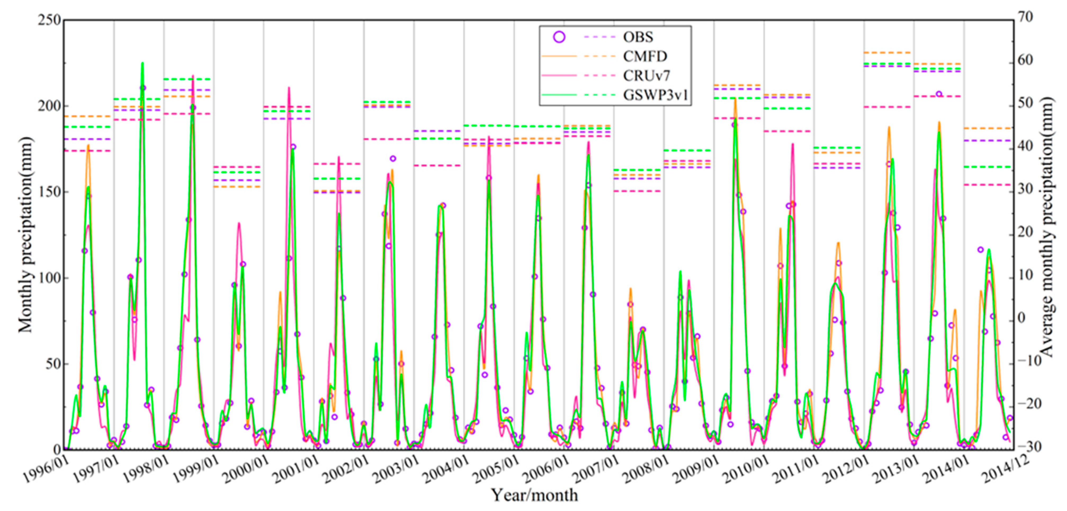
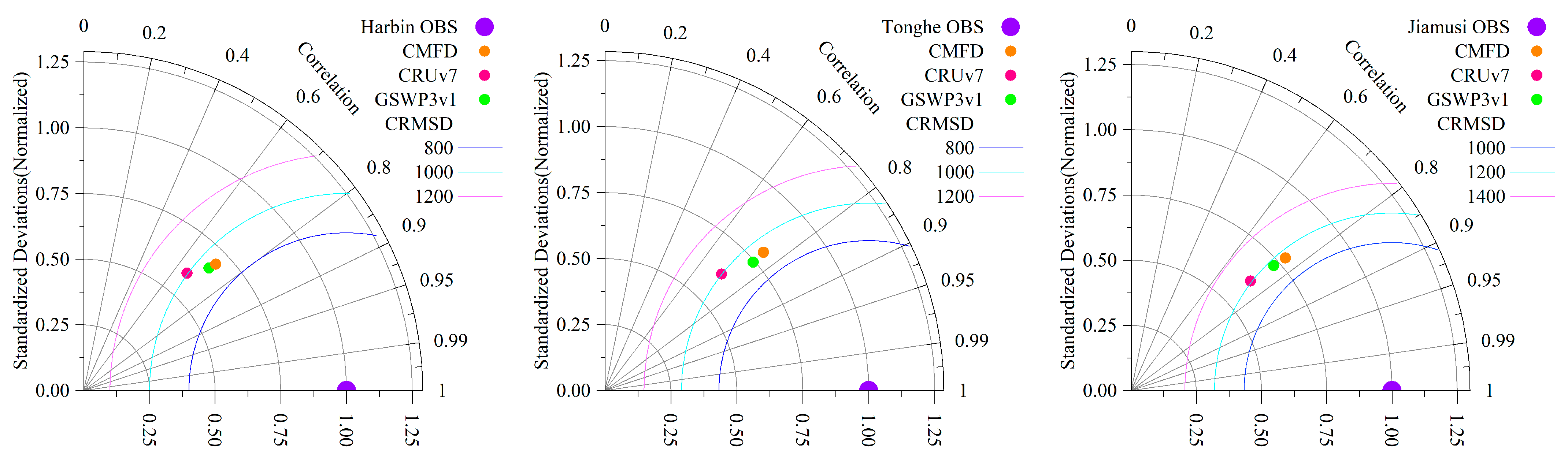
3.1. Evaluation of Precipitation in Meteorological Forcing Data

In this study, we compared the quality of precipitation data in different meteorological forcing data by calculating the average monthly precipitation from 1996 to 2014 in the basin (AMPB) and the average monthly precipitation during the year (AMPY) from three standardized stations in the basin. As shown in Figure 3, CRUv7 underestimated precipitation, which exhibited poor performance, and both CMFD and GSWP3v1 overestimated precipitation. CRUv7 underestimated precipitation for 1996–1998, 2002–2003, 2005–2007, 2009–2010, and 2012–2014; the resolution of CRU v7 is 0.5°, but meteorological stations can represent precipitation only within several kilometers around the observation point, limited in spatial and temporal coverage, because of the large single-point observational errors [9,47]. AMPB underestimated precipitation by an average of 11.2 mm, and AMPY underestimated precipitation by an average of 5.4 mm, the overall precipitation trends differed from the other data. The results suggested that CRUv7 was less applicable in the SRB than in previous study areas [48]. CMFD and GSWP3v1 showed overestimation of precipitation, with a slightly more pronounced overestimation for GSWP3v1. For GSWP3v1, AMPB was overestimated by an average of 6.5 mm, and AMPY was overestimated by an average of 2.4 mm. For CMFD, AMPB was overestimated by an average of 4.6 mm and AMPY by an average of 1.8 mm; while from

Table 3. Multi-station precipitation comparison across time scales (unit: mm).

Datasets	Day	Jan	Feb	Mar	Apr	May	Jun	Jul	Aug	Sept	Oct	Nov	Dec	Year
OBS	1.46	5.71	4.99	15.25	22.93	55.18	83.05	125.14	118.66	47.61	29.08	16.74	9.59	533.92
CMFD	1.50	6.31	4.90	15.40	23.22	60.26	88.27	127.73	119.28	47.35	28.24	17.08	9.29	547.33
CRUv7	1.37	3.89	4.00	13.15	26.81	52.21	82.95	131.90	107.28	38.36	22.28	10.88	5.96	499.67
GSWP3v1	1.50	6.19	5.60	17.82	28.47	53.04	92.15	130.04	120.03	42.18	27.74	17.31	8.59	549.15

, CMFD underestimated precipitation in the cool season and overestimated precipitation in the warm season, which was consistent with previous studies on the Tibetan Plateau [49].

To further understand the data quality of the three datasets under different precipitation intensities (PI, mm/d), the PI was categorized into seven groups (0 ≤ PI < 1, 1 ≤ PI < 5, 5 ≤ PI < 10, 10 ≤ PI < 20, 20 ≤ PI < 30, 30 ≤ PI < 50, PI > 50) in this study. Figure 4 shows the total precipitation for the three datasets from 1996 to 2014 under different PI groups. The analysis results showed that the overestimation of precipitation in CRUv7 was mainly concentrated in the range of PI = 1~10 mm/d, and there was underestimation of precipitation in CRUv7 in the group with PI ≥ 10 mm/d. GSWP3v1 and CMFD were closer to the observations (OBS, data from stations) than CRUv7 in all PI groups, but in the low-intensity precipitation (PI = 0~10 mm/d) range, both overestimated precipitation, and in the high-intensity precipitation (PI > 10 mm/d) range, GSWP3v1 and CMFD generally underestimated precipitation. The results of total precipitation in different PI ranges showed only the overestimation and underestimation of precipitation; however, they could not represent the accuracy of precipitation products in detecting actual precipitation. Therefore, in this study, the precipitation products were further grouped according to the PI of OBS, and then the CC and RMSE were calculated for each precipitation dataset with different PI intervals. The results are shown in

Table 4. Comparison of different PI groups: statistical overview of multiple precipitation products against OBS.

PI (mm/d)	CMFD		CRUv7		GSWP3v1
	CC	RMSE	CC	RMSE	CC	RMSE
[0, 1)	0.34	0.22	0.09	0.23	0.03	0.23
[1, 5)	0.37	1.00	0.13	1.13	0.02	1.13
[5, 10)	0.23	1.37	0.02	1.35	0.12	1.42
[10, 20)	0.27	2.71	0.04	2.37	0.11	3.01
[20, 30)	0.06	2.35	−0.12	2.75	0.17	2.81
[30, +∞)	0.48	5.90	−0.59	6.19	−0.08	12.08

. At different PI intervals, Table 4 shows that the correlation between CMFD and OBS was the highest and the RMSE was the smallest, and the most accurate estimation of precipitation was found when 30 ≤ PI, with an RMSE of 5.90 mm, followed by 0 ≤ PI < 1, with an RMSE of 0.22 mm.

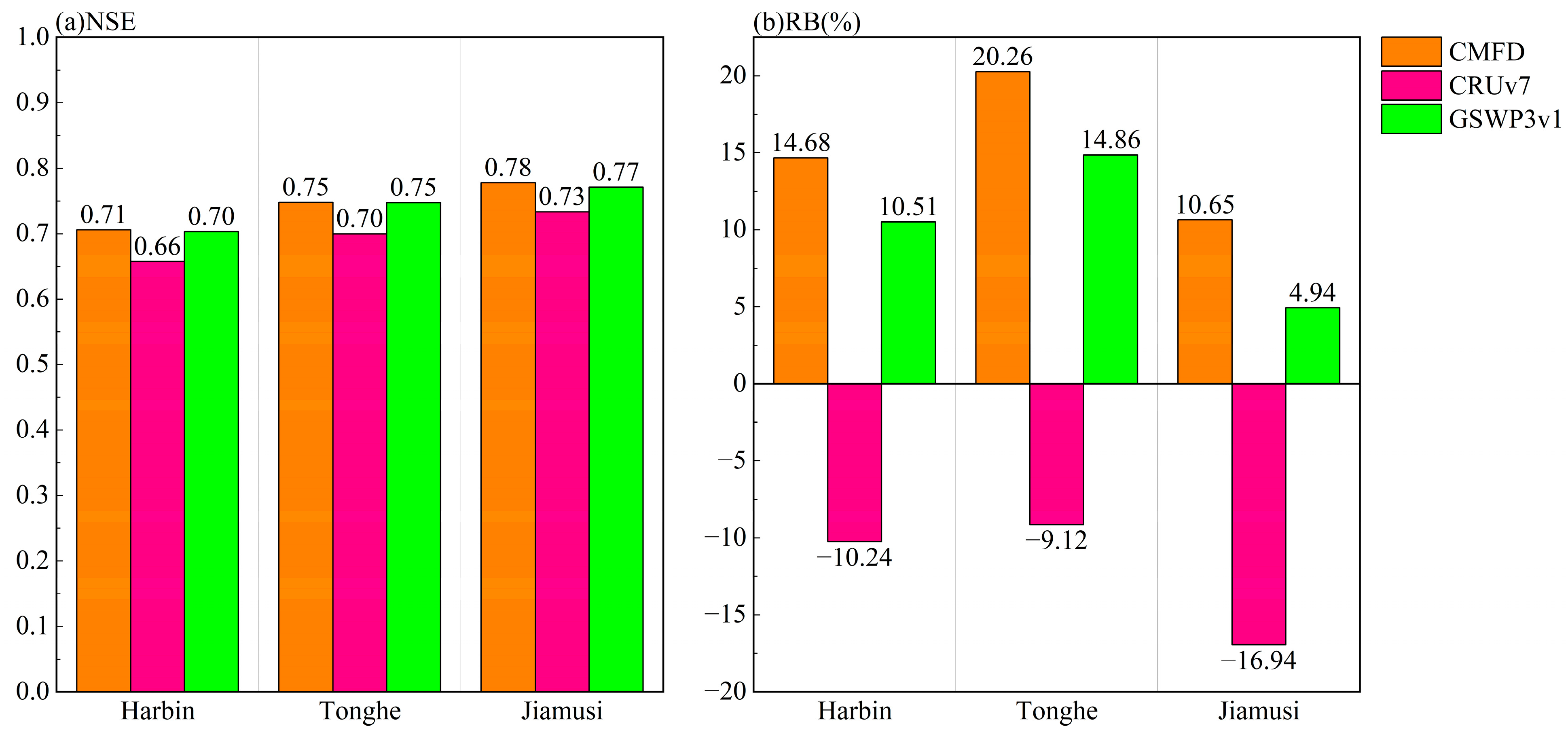
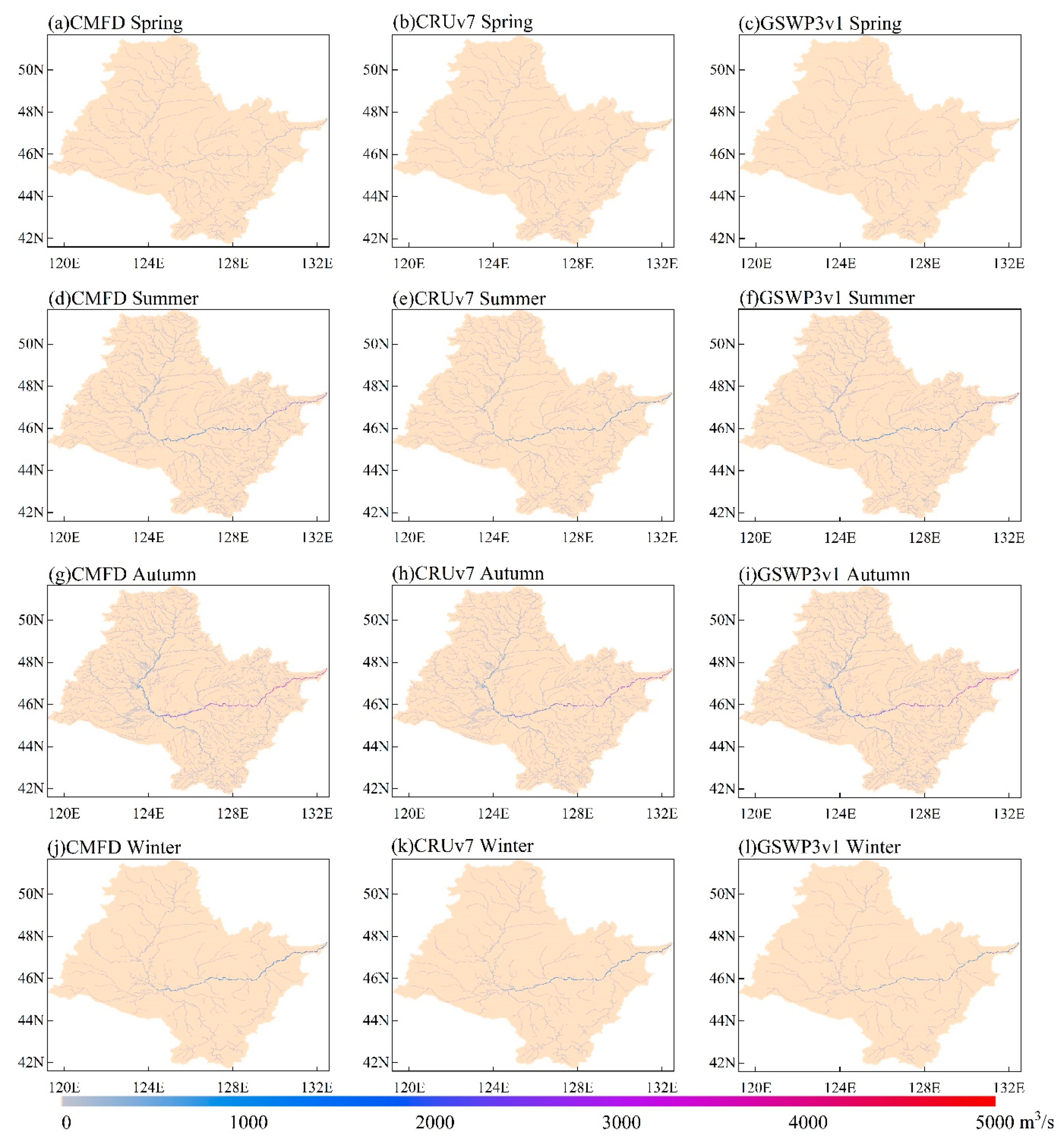
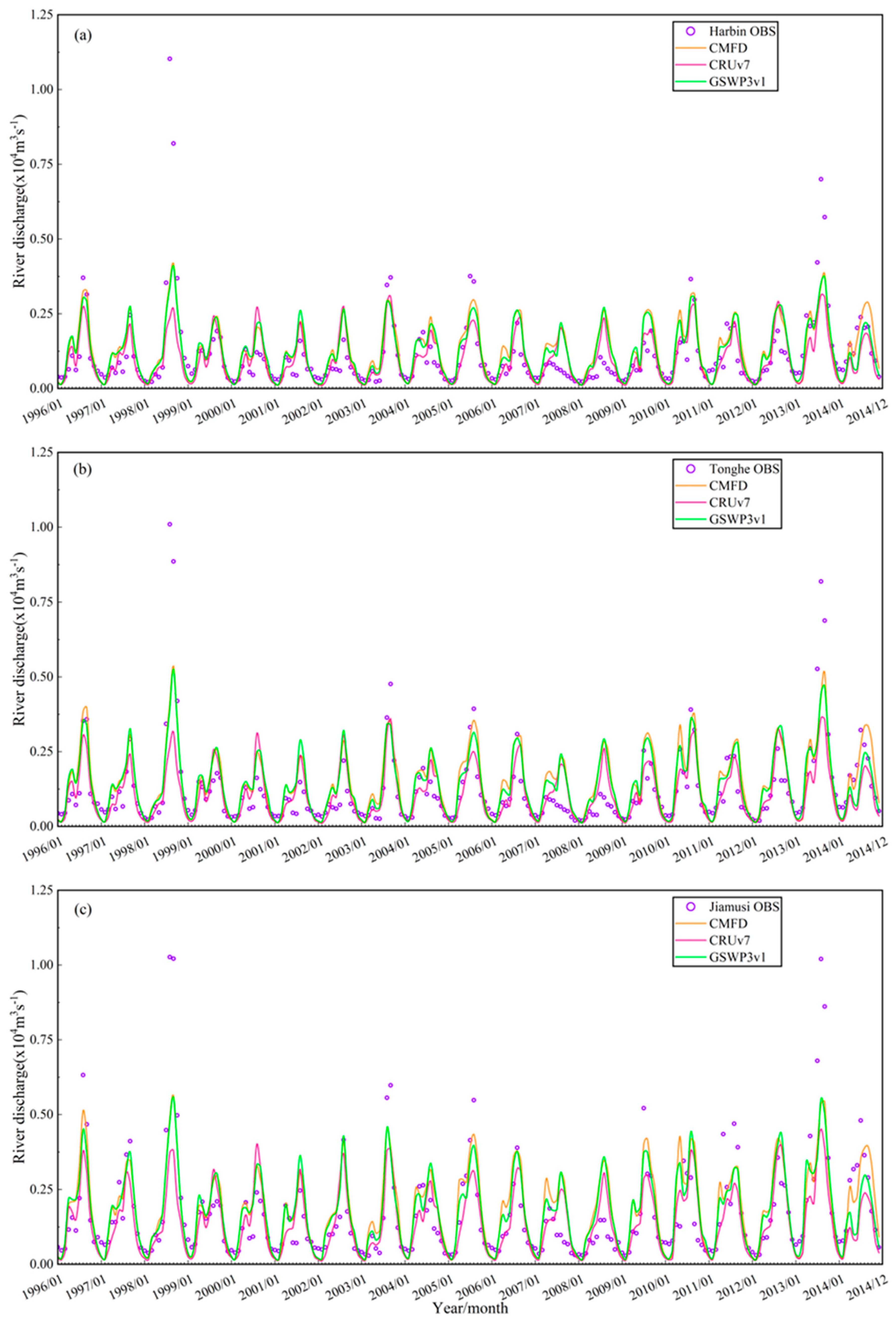
3.2. Evaluation of Discharge

In this study, we obtained the average spatial pattern of the SRB for the period 1996–2014 by combining the CaMa-Flood with three datasets of 0.1° × 0.1° runoff obtained from the coupled simulation of CLM5, which represented the dynamic hydrological processes at a high spatial resolution of 1′ × 1′ and spatially captured the flood flow in autumn and the river recession process in winter in the SRB. Figure 5 shows the seasonal cycle of the simulated discharge during 1996–2014, with a clear ground flood evolution along the SRB from upstream to downstream. The seasonal variation in the simulated flooded area during the period 1996–2014 is illustrated in Figure 6, with a clear exposure to a more severe flood risk during the warm season in the SRB. The performance of the simulated seasonal discharge is demonstrated in Figure 7, which varied depending on the meteorological forcing data, station location, and different rivers in the basin, as shown at the Harbin, Tonghe, and Jiamusi hydrological stations (Figure 2). Comparing the simulated discharge with the OBS at the hydrological stations, in the middle and lower reaches of the SRB, the simulated discharge agreed with the measured discharge in most of the period, and the simulated discharge could override the observed discharge, but during the 1998 and 2013 warm seasons, CMFD, GSWP3v1, and CRUv7 all significantly underestimated the peak discharge, and all three overestimated the discharge in the 2007 and 2008 warm seasons. The interannual variations described by the coefficients of variation (CVs) of the simulated and measured discharge during 1996–2014 are compared in Figure 8. The three datasets of discharge simulations at Harbin, Tonghe, and Jiamusi stations agreed with the CVs of the observed discharge in the cold season, and the simulated discharge significantly underestimated the CVs of the observed discharge in the warm season.

The Taylor plot in Figure 9 summarizes the centered root-mean-square difference (CRMSD), normalized standard deviation (STD), and CC between simulated and OBS daily flows for the period 1996–2014. The CRMSD values consistently exhibit higher magnitudes for Jiamusi station compared to Harbin and Tonghe stations, signifying a relatively diminished accuracy in the simulated discharge outcomes for Jiamusi. No significant difference is observed in the simulated discharge performance between Harbin and Tonghe stations. All simulated discharge STDs were less than 1, with CMFD simulations yielding discharge STDs closest to 1; GSWP3v1 is the next closest, and CRUv7 is the worst. Most of the CC values ranged from 0.65 to 0.80, with the highest correlation between simulated and measured discharge for CMFD at Jiamusi station and GSWP3v1 at Tonghe station, both with CC values of 0.76 (p < 0.01), and the poorest fit of simulated discharge to observed discharge for CRUv7 at Harbin station, with a CC value of 0.66 (p < 0.01). From the results, the discharge obtained from the CMFD simulation had more points close to the observed data, which was more suitable for the SRB than GSWP3v1 with CRUv7, which was consistent with the results of the analysis and evaluation of precipitation data in Section 3.1.

Figure 10a depicts the NSE of the daily-scale simulated and observed discharges for the period of 1996–2014, and the values of the simulated daily discharges obtained from the three meteorological forcing datasets simulated by the coupled model with the NSE calculated from the measured daily discharges were all greater than 0.6, which implied that the meteorological forcing data combined with CLM5 and CaMa-Flood v4.1 simulated the discharge process better in the SRB. Among them, CMFD performed the best, with the highest NSE value at Jiamusi station (0.78) and the lowest NSE value at Harbin station (0.71), and the mean NSE value of CMFD was 0.74. Similar to CMFD, GSWP3v1 and CRUv7 had the lowest NSE values at Harbin station, which were 0.70 and 0.66, respectively, and the mean NSE values of both were 0.74 (slightly lower than that of CMFD) and 0.70, respectively. In summary, the flow simulation of CMFD was better than that of GSWP3v1 and CRUv7. The difference here may be attributed to the meteorological forcing data uncertainty, model uncertainty, and the interaction between model uncertainty and meteorological forcing data uncertainty. Figure 10b depicts the RBs of the daily-scale simulated and observed discharges for the period 1996–2014. The RBs of the simulated daily discharges obtained by the coupled model simulations at the three hydrological stations by CMFD and GSWP3v1 and the calculated RBs of the measured daily discharges were both greater than 0, and the RBs of CRUv7 were both less than 0, i.e., the discharges in the SRB were overestimated by CMFD and GSWP3v1, and the discharges in the SRBs were underestimated by CRUv7. For discharges, CMFD and GSWP3v1 had the highest uncertainty at Tonghe station, with RB values as high as 20.26% and 14.86%, respectively, and both had the lowest uncertainty at Jiamusi station, with RB values of 10.65% and 4.94%, respectively. CRUv7 was the opposite of the former two, which had the lowest uncertainty at Tonghe station (−9.12%) and the highest at Jiamusi (−16.94%). The mean absolute RB values of CMFD, GSWP3v1, and CRUv7 were 15.2%, 10.1%, and 12.1%, respectively. GSWP3v1 was closer to the measured discharges than CMFD and CRUv7, but it still had some uncertainty. The underestimation of the discharge by CRUv7 was probably due to its underestimation of the high-intensity precipitation (Figure 4).

4. Discussion

4.1. Impact of Precipitation Data on Discharge

In the comparison analysis of each station, we evaluated the accuracy of CMFD, CRUv7, and GSWP3v1 in recording precipitation in the SRB from 1996 to 2014 based on precipitation data obtained from meteorological stations. The results showed that the precipitation trends of the CMFD were the most similar to the trends of OBS at the yearly, monthly, and daily scales. The better performance of CMFD precipitation was attributed to its integration with CMA, in addition to the fact that the spatial resolution of CMFD is higher than that of both CRUv7 and GSWP3v1, which further improves the accuracy of the precipitation data within the SRB. Experiments conducted on the evaluation of meteorological forcing data on the Yunnan-Guizhou Plateau and throughout China also showed that CMFD and GSWP3v1 yielded better results than CRUv7 as forcing data [50]. From Table 4, it can be seen that in the range of medium- to high-intensity precipitation (PI > 10 mm/d), the RSME of CMFD, CRUv7, and GSWP3v1 goes from 2.35 mm/d to 12.08 mm/d, which is much larger than the RMSE (0.22~1.42 mm/d) of low-intensity precipitation (0 ≤ PI < 10 mm/d), and considering that most of the moderate to heavy precipitation in the SRB occurs in the warm season [24], this result demonstrates that all precipitation data are insufficient to monitor short-term high-intensity precipitation. However, meteorological forcing data contain information at a larger spatial resolution, representing the meteorological conditions in the area covered by the scale, and the observations contain only the real values at this point of the standardized station [51]. This shortcoming is reflected in the discharge simulation results of the model, and the CVs of monthly discharges in Figure 8 show that the simulated discharge fluctuates to a lesser extent than the observed discharge during the cold season in the time period under study, and the value of the CVs is generally in the range of 0.1–0.5. The observed discharge fluctuation in the SRB in the warm season is high throughout the year, and the value of the CVs is generally in the range of 0.6–1.0, while that of the CVs of the simulated discharge is mostly in the range of 0.1–0.4 in the warm season, and the model is not sufficiently accurate to simulate the discharge in the warm season, which makes the simulated discharge differ from the data of the hydrological stations in Harbin, Tonghe, and Jiamusi in the warm seasons of 1996 and 2013—sufficient reason to determine that the meteorological forcing data are deficient in their ability to capture medium- and high-intensity precipitation data in the warm season.

Precipitation is very critical for discharge simulation [51], and the regional discharge simulations performed in this study relied heavily on precipitation data input to CLM5. Precipitation data error is affected by satellites’ sensor types and inversion algorithms, and analyzing and evaluating the precipitation data in CMFD, CRUv7, and GSWP3v1 does not provide information on which sensor type and inversion algorithm can be used to improve discharge simulation in the SRB. Therefore, future research could focus on comparing all precipitation products using different sensor types and inversion algorithms with CMFD, CRUv7, and GSWP3v1, which would enhance the discharge simulation capability of CLM5 in the SRB after improving the hydrologic postprocessing routine and provide a basis for higher resolution discharge and flooded area simulations.

4.2. Considerations and Potential Implications for Model Improvement

Studies in arid and semiarid regions have shown that the runoff and river evolution performance of CLM is not satisfactorily improved by parameter calibration [52], so we improved it by introducing physically based runoff and river evolution schemes. From the simulation results of the discharge and flooded areas from 1996 to 2014 (Figure 5 and Figure 6), this study better restored the high-resolution dynamic hydrological processes in the SRB and provided high-resolution discharge datasets and inundation area maps through an offline coupling model with strong physical mechanisms. The NSE of the present simulated daily discharge to station observations ranges from 0.72 ± 0.06, and the RB of daily discharge simulated by GSWP3v1 ranges from 4.94% to 14.86%. Spatially, the higher topography in the southeast and northwest of the SRB results in some areas in the middle and lower reaches of the SRB being permanently flooded, which could be exposed to a greater risk of flooding during the warm season.

The spatial and temporal heterogeneity of surface runoff is driven by a sophisticated mixture of climate change and anthropogenic factors, with multiple drivers overlapping. The consideration of anthropogenic factors in the simulation framework proposed in this study is primarily illustrated by the consideration that the subsurface data in CLM5 is a dynamically varying dataset encompassing a wide number of PFTs, but in a high-latitude SRB with snow and precipitation, we also need to estimate LSMs under the combined influence of different PFTs and reanalysis products, which can be used to model the water fluxes with more accuracy. Based on the rapid development of machine learning and artificial intelligence in the field of climate forecasting and simulation, the accuracy of the meteorological forcing data mass has been substantially enhanced [53,54]. The modeling framework presented in this research can be used as a postprocessing approach to decrease the forecastable bias of the numerical weather prediction, and the high-quality meteorological forcing data provide the foundation of the modified CLM5, which can be applied to the high-resolution discharge modeling and prediction of the SRB.

5. Conclusions

In this study, we quantified the overall performance of SRB discharge estimates obtained from different meteorological forcing datasets simulated by offline coupling CLM5 with CaMa-Flood. Three high-resolution discharge datasets were obtained by inputting three meteorological forcing datasets from 1996–2014, combined with SRB’s high-resolution subsurface dataset, into CLM5 for land surface process simulation, followed by offline coupling CaMa-Flood for confluence process simulation of river discharge from 1996 to 2014. The major conclusions of this study are as follows. First, the results of the quantitative assessment of the precipitation data showed that in the SRB, CMFD exhibited the highest quality, followed by GSWP3v1, while CRUv7 performed the least effectively. Notably, all three datasets exhibited limited capability to capture high-intensity precipitation events. Second, both discharge and flooded areas simulated based on the coupled model showed good seasonality, spatially capturing the process of river discharge increase in the warm season and river recession in the cold season. Furthermore, simulating the multi-year average flooded area within the SRB based on runoff showed the ability to monitor flooding. Third, the discharges simulated by the coupled model were validated by comparison with the actual measurements, and the best-performing CMFDs in the Taylor diagrams had higher NSEs at Harbin Station (0.71), Tonghe Station (0.75), and Jiamusi Station (0.78). In addition, the fluctuation range of the simulated discharges generally covers the measured data.

The findings of this study provide a foundation for the application of offline coupling land surface models with hydrological models in flood monitoring and early warning systems. Compared to the flow observation data at the SRB hydrostations, the coupled model simulations exhibit similar spatial patterns. However, due to the inadequate capacity of meteorological datasets to observe short-term intensive precipitation, the discharge during the warm season is largely underestimated [55]. Therefore, prior to application, it is necessary to optimize meteorological data, especially the precipitation component, to achieve reliable simulation results. Furthermore, the low resolution of the subsurface dataset restricts the resolution of the coupled model simulation results. More precise flood risk maps can only be generated by identifying potential flood inundation areas and integrating them with high-intensity rainfall events.

Because the offline coupling model of CLM5 and CaMa-Flood possesses a robust physical mechanism and is relatively insensitive to parameter adjustments [52], its applicability in other regions is assured. This coupled model can be employed to simulate runoff processes in medium and large global basins under varying climate scenarios, aiding in enhancing our understanding of runoff processes under different climate scenarios. The simulation results of inundated areas can serve as a reference for decision-makers in formulating plans to address flooding.

References

1. Yin, J.; Gentine, P.; Zhou, S.; Sullivan, S.C.; Wang, R.; Zhang, Y.; Guo, S. Large increase in global storm runoff extremes driven by climate and anthropogenic changes. Nat. Commun. 2018, 9, 4389. [Google Scholar] [CrossRef]
2. Miao, Y.; Wang, A. Evaluation of Routed-Runoff from Land Surface Models and Reanalyses Using Observed Streamflow in Chinese River Basins. J. Meteorol. Res. 2020, 34, 73–87. [Google Scholar] [CrossRef]
3. Vergara-Temprado, J.; Ban, N.; Schär, C. Extreme Sub-Hourly Precipitation Intensities Scale Close to the Clausius-Clapeyron Rate Over Europe. Geophys. Res. Lett. 2021, 48, e2020gl089506. [Google Scholar] [CrossRef]
4. Piao, S.; Ciais, P.; Huang, Y.; Shen, Z.; Peng, S.; Li, J.; Zhou, L.; Liu, H.; Ma, Y.; Ding, Y.; et al. The impacts of climate change on water resources and agriculture in China. Nature 2010, 467, 43–51. [Google Scholar] [CrossRef]
5. Cui, T.; Li, Y.; Yang, L.; Nan, Y.; Li, K.; Tudaji, M.; Tian, F. Non-monotonic changes in Asian Water Towers’ streamflow at increasing warming levels. Nat. Commun. 2023, 14, 1176. [Google Scholar] [CrossRef] [PubMed]
6. Rosa, L.; Chiarelli, D.D.; Rulli, M.C.; Dell’Angelo, J.; D’Odorico, P. Global agricultural economic water scarcity. Sci. Adv. 2020, 6, eaaz6031. [Google Scholar] [CrossRef] [PubMed]
7. Qi, W.; Feng, L.; Yang, H.; Zhu, X.; Liu, Y.; Liu, J. Weakening flood, intensifying hydrological drought severity and decreasing drought probability in Northeast China. J. Hydrol. Reg. Stud. 2021, 38, 100941. [Google Scholar] [CrossRef]
8. Qi, W.; Liu, J.; Yang, H.; Zhu, X.; Tian, Y.; Jiang, X.; Feng, L. Large Uncertainties in Runoff Estimations of GLDAS Versions 2.0 and 2.1 in China. Earth Space Sci. 2020, 7, e2019ea000829. [Google Scholar] [CrossRef]
9. Qi, W.; Zhang, C.; Fu, G.; Zhou, H. Global Land Data Assimilation System data assessment using a distributed biosphere hydrological model. J. Hydrol. 2015, 528, 652–667. [Google Scholar] [CrossRef]
10. Zaitchik, B.F.; Rodell, M.; Olivera, F. Evaluation of the Global Land Data Assimilation System using global river discharge data and a source-to-sink routing scheme. Water Resour. Res. 2010, 46, W06507. [Google Scholar] [CrossRef]
11. Massoud, E.C.; Bloom, A.A.; Longo, M.; Reager, J.T.; Levine, P.A.; Worden, J.R. Information content of soil hydrology in a west Amazon watershed as informed by GRACE. Hydrol. Earth Syst. Sci. 2022, 26, 1407–1423. [Google Scholar] [CrossRef]
12. Xiong, J.; Guo, S.; Yin, J.; Gu, L.; Xiong, F. Using the Global Hydrodynamic Model and GRACE Follow-On Data to Access the 2020 Catastrophic Flood in Yangtze River Basin. Remote Sens. 2021, 13, 3023. [Google Scholar] [CrossRef]
13. Zhang, X.-J.; Tang, Q.; Pan, M.; Tang, Y. A Long-Term Land Surface Hydrologic Fluxes and States Dataset for China. J. Hydrometeorol. 2014, 15, 2067–2084. [Google Scholar] [CrossRef]
14. Sellers, P.J.; Dickinson, R.E.; Randall, D.A.; Betts, A.K.; Hall, F.G.; Berry, J.A.; Henderson-Sellers, A. Modeling the Exchanges of Energy, Water, and Carbon Between Continents and the Atmosphere. Science 1997, 275, 502–509. [Google Scholar] [CrossRef]
15. Mitchell, K.E. The multi-institution North American Land Data Assimilation System (NLDAS): Utilizing multiple GCIP products and partners in a continental distributed hydrological modeling system. J. Geophys. Res. 2004, 109, D07S90. [Google Scholar] [CrossRef]
16. Danabasoglu, G.; Lamarque, J.F.; Bacmeister, J.; Bailey, D.A.; DuVivier, A.K.; Edwards, J.; Strand, W.G. The Community Earth System Model Version 2 (CESM2). J. Adv. Model. Earth Syst. 2020, 12, e2019ms001916. [Google Scholar] [CrossRef]
17. Lawrence, D.M.; Oleson, K.W.; Flanner, M.G.; Thornton, P.E.; Swenson, S.C.; Lawrence, P.J.; Slater, A.G. Parameterization improvements and functional and structural advances in Version 4 of the Community Land Model. J. Adv. Model. Earth Syst. 2011, 3, e2011ms000045. [Google Scholar] [CrossRef]
18. Oleson, K.; Lawrence, D.M.; Bonan, G.B.; Drewniak, B.; Huang, M.; Koven, C.D.; Levis, S.; Li, F.; Riley, W.J.; Subin, Z.M.; et al. Technical Description of Version 4.5 of the Community Land Model (CLM) (No. NCAR/TN-503+STR); National Center for Atmospheric Research: Boulder, CO, USA, 2013. [Google Scholar] [CrossRef]
19. Berghuijs, W.R.; Harrigan, S.; Molnar, P.; Slater, L.J.; Kirchner, J.W. The Relative Importance of Different Flood-Generating Mechanisms Across Europe. Water Resour. Res. 2019, 55, 4582–4593. [Google Scholar] [CrossRef]
20. Yamazaki, D.; Kanae, S.; Kim, H.; Oki, T. A physically based description of floodplain inundation dynamics in a global river routing model. Water Resour. Res. 2011, 47, W04501. [Google Scholar] [CrossRef]
21. Faiz, M.A.; Liu, D.; Fu, Q.; Uzair, M.; Khan, M.I.; Baig, F.; Cui, S. Stream flow variability and drought severity in the Songhua River Basin, Northeast China. Stoch. Environ. Res. Risk Assess. 2017, 32, 1225–1242. [Google Scholar] [CrossRef]
22. Wang, S.; Wang, Y.; Ran, L.; Su, T. Climatic and anthropogenic impacts on runoff changes in the Songhua River basin over the last 56years (1955–2010), Northeastern China. Catena 2015, 127, 258–269. [Google Scholar] [CrossRef]
23. Yu, C.; Shao, H.; Hu, D.; Liu, G.; Dai, X. Merging precipitation scheme design for improving the accuracy of regional precipitation products by machine learning and geographical deviation correction. J. Hydrol. 2023, 620, 129560. [Google Scholar] [CrossRef]
24. Chen, J.; Liao, J. Monitoring lake level changes in China using multi-altimeter data (2016–2019). J. Hydrol. 2020, 590, 125544. [Google Scholar] [CrossRef]
25. Chen, J.; Fenoglio, L.; Kusche, J.; Liao, J.; Uyanik, H.; Nadzir, Z.A.; Lou, Y. Evaluation of Sentinel-3A altimetry over Songhua river Basin. J. Hydrol. 2023, 618, 129197. [Google Scholar] [CrossRef]
26. Wu, Y.; Ju, H.; Qi, P.; Li, Z.; Zhang, G.; Sun, Y. Increasing flood risk under climate change and social development in the Second Songhua River basin in Northeast China. J. Hydrol. Reg. Stud. 2023, 48, 101459. [Google Scholar] [CrossRef]
27. He, J.; Yang, K.; Tang, W.; Lu, H.; Qin, J.; Chen, Y.; Li, X. The first high-resolution meteorological forcing dataset for land process studies over China. Sci. Data 2020, 7, 25. [Google Scholar] [CrossRef] [PubMed]
28. Peng, J.M.; Liu, S.F.; Dai, Y.J.; Wei, N. Evaluation of Common Land Model Based on International Land Model Benchmarking System. Clim. Environ. Res. 2020, 25, 649–666. [Google Scholar] [CrossRef]
29. Kim, H.J. Global Soil Wetness Project Phase 3 Atmospheric Boundary Counditions (Experiment 1); Data Integration and Analysis System (DIAS): Tokyo, Japan, 2017. [Google Scholar] [CrossRef]
30. Viovy, N. CRUNCEP Version 7—Atmospheric Forcing Data for the Community Land Model; Research Data Archive at the National Center for Atmospheric Research, Computational and Information Systems Lab: Boulder, CO, USA, 2018. [Google Scholar] [CrossRef]
31. Yu, Z.; Lu, C.; Tian, H.; Canadell, J.G. Largely underestimated carbon emission from land use and land cover change in the conterminous United States. Glob. Chang. Biol. 2019, 25, 3741–3752. [Google Scholar] [CrossRef]
32. Loveland, T.R.; Reed, B.C.; Brown, J.F.; Ohlen, D.O.; Zhu, Z.; Yang, L.; Merchant, J.W. Development of a global land cover characteristics database and IGBP DISCover from 1 km AVHRR data. Int. J. Remote Sens. 2010, 21, 1303–1330. [Google Scholar] [CrossRef]
33. Lawrence, P.J.; Chase, T.N. Representing a new MODIS consistent land surface in the Community Land Model (CLM 3.0). J. Geophys. Res. 2007, 112, G01023. [Google Scholar] [CrossRef]
34. Klein Goldewijk, K.; Beusen, A.; Doelman, J.; Stehfest, E. Anthropogenic land use estimates for the Holocene—HYDE 3.2. Earth Syst. Sci. Data 2017, 9, 927–953. [Google Scholar] [CrossRef]
35. Lawrence, D.M.; Hurtt, G.C.; Arneth, A.; Brovkin, V.; Calvin, K.V.; Jones, A.D.; Shevliakova, E. The Land Use Model Intercomparison Project (LUMIP) contribution to CMIP6: Rationale and experimental design. Geosci. Model Dev. 2016, 9, 2973–2998. [Google Scholar] [CrossRef]
36. Yamazaki, D.; Ikeshima, D.; Sosa, J.; Bates, P.D.; Allen, G.H.; Pavelsky, T.M. MERIT Hydro: A High-Resolution Global Hydrography Map Based on Latest Topography Dataset. Water Resour. Res. 2019, 55, 5053–5073. [Google Scholar] [CrossRef]
37. Wigmosta, M.S.; Li, H.; Wu, H.; Huang, M.; Ke, Y.; Coleman, A.M.; Leung, L.R. A Physically Based Runoff Routing Model for Land Surface and Earth System Models. J. Hydrometeorol. 2013, 14, 808–828. [Google Scholar] [CrossRef]
38. Lawrence, D.M.; Fisher, R.A.; Koven, C.D.; Oleson, K.W.; Swenson, S.C.; Bonan, G.; Zeng, X. The Community Land Model Version 5: Description of New Features, Benchmarking, and Impact of Forcing Uncertainty. J. Adv. Model. Earth Syst. 2019, 11, 4245–4287. [Google Scholar] [CrossRef]
39. Niu, G.-Y.; Yang, Z.-L.; Dickinson, R.E.; Gulden, L.E. A simple TOPMODEL-based runoff parameterization (SIMTOP) for use in global climate models. J. Geophys. Res. 2005, 110, D21106. [Google Scholar] [CrossRef]
40. Tesfa, T.K.; Li, H.Y.; Leung, L.R.; Huang, M.; Ke, Y.; Sun, Y.; Liu, Y. A subbasin-based framework to represent land surface processes in an Earth system model. Geosci. Model Dev. 2014, 7, 947–963. [Google Scholar] [CrossRef]
41. Verdin, K.L.; Jenson, S.K. Development of Continental Scale Digital Elevation Models and Extraction of Hydrographic Features. In Proceedings of the Third International Conference/Workshop on Integrating GIS and Environmental Modeling, Sante Fe, NM, USA, 21–25 January 1996; pp. 397–403. [Google Scholar]
42. Yamazaki, D.; Ikeshima, D.; Tawatari, R.; Yamaguchi, T.; O’Loughlin, F.; Neal, J.C.; Bates, P.D. A high-accuracy map of global terrain elevations. Geophys. Res. Lett. 2017, 44, 5844–5853. [Google Scholar] [CrossRef]
43. Yamazaki, D.; Lee, H.; Alsdorf, D.E.; Dutra, E.; Kim, H.; Kanae, S.; Oki, T. Analysis of the water level dynamics simulated by a global river model: A case study in the Amazon River. Water Resour. Res. 2012, 48, W09508. [Google Scholar] [CrossRef]
44. Yamazaki, D.; Oki, T.; Kanae, S. Deriving a global river network map and its sub-grid topographic characteristics from a fine-resolution flow direction map. Hydrol. Earth Syst. Sci. 2009, 13, 2241–2251. [Google Scholar] [CrossRef]
45. Rojas, M.; Lambert, F.; Ramirez-Villegas, J.; Challinor, A.J. Emergence of robust precipitation changes across crop production areas in the 21st century. Proc. Natl. Acad. Sci. USA 2019, 116, 6673–6678. [Google Scholar] [CrossRef] [PubMed]
46. Yang, H.; Zhou, F.; Piao, S.; Huang, M.; Chen, A.; Ciais, P.; Zeng, Z. Regional patterns of future runoff changes from Earth system models constrained by observation. Geophys. Res. Lett. 2017, 44, 5540–5549. [Google Scholar] [CrossRef]
47. He, Z.; Hu, H.; Tian, F.; Ni, G.; Hu, Q. Correcting the TRMM rainfall product for hydrological modelling in sparsely-gauged mountainous basins. Hydrol. Sci. J. 2016, 62, 306–318. [Google Scholar] [CrossRef]
48. Cao, Y.; Fu, C.; Wang, X.; Dong, L.; Yao, S.; Xue, B.; Wu, H. Decoding the dramatic hundred-year water level variations of a typical great lake in semi-arid region of northeastern Asia. Sci. Total Environ. 2021, 770, 145353. [Google Scholar] [CrossRef]
49. Zhang, L.; Gao, L.; Chen, J.; Zhao, L.; Zhao, J.; Qiao, Y.; Shi, J. Comprehensive evaluation of mainstream gridded precipitation datasets in the cold season across the Tibetan Plateau. J. Hydrol. Reg. Stud. 2022, 43, 101186. [Google Scholar] [CrossRef]
50. Yu, H.; Wang, L.; Yang, M. Effects of Elevation and Longitude on Precipitation and Drought on the Yunnan–Guizhou Plateau, China. Pure Appl. Geophys. 2023, 180, 2461–2481. [Google Scholar] [CrossRef]
51. Bodjrènou, R.; Sintondji, L.O.; Comandan, F. Hydrological modeling with physics-based models in the oueme basin: Issues and perspectives for simulation optimization. J. Hydrol. Reg. Stud. 2023, 48, 101448. [Google Scholar] [CrossRef]
52. Sheng, M.; Lei, H.; Jiao, Y.; Yang, D. Evaluation of the Runoff and River Routing Schemes in the Community Land Model of the Yellow River Basin. J. Adv. Model. Earth Syst. 2017, 9, 2993–3018. [Google Scholar] [CrossRef]
53. Bi, K.; Xie, L.; Zhang, H.; Chen, X.; Gu, X.; Tian, Q. Accurate medium-range global weather forecasting with 3D neural networks. Nature 2023, 619, 533–538. [Google Scholar] [CrossRef]
54. Hu, Y.; Chen, L.; Wang, Z.; Li, H. SwinVRNN: A Data-Driven Ensemble Forecasting Model via Learned Distribution Perturbation. J. Adv. Model. Earth Syst. 2023, 15, e2022ms003211. [Google Scholar] [CrossRef]
55. Wang, L.; Zhang, F.; Zhang, H.; Scott, C.A.; Zeng, C.; Shi, X. Intensive precipitation observation greatly improves hydrological modelling of the poorly gauged high mountain Mabengnong catchment in the Tibetan Plateau. J. Hydrol. 2018, 556, 500–509. [Google Scholar] [CrossRef]
Figure 1. Map of subbasins and river networks within the SRB.
Water 16 00442 g001
Figure 2. Flowchart of the offline coupling model CLM5 and CaMa-Flood v4.1.
Water 16 00442 g002
Figure 3. Exploring multi-station perspectives: a comparative study of the average monthly precipitation in the basin (solid lines) and the average monthly precipitation during the year (dashed lines).
Water 16 00442 g003
Figure 4. Precipitation in different PI groups from 1996 to 2014.
Water 16 00442 g004
Figure 5. Seasonal spatial distribution of ensemble means of discharge between 1996 and 2014.
Water 16 00442 g005
Figure 6. Seasonal spatial distribution of ensemble means of flooded areas between 1996 and 2014.
Water 16 00442 g006
Figure 7. Comparisons of monthly observed and simulated discharge during 1996–2014 at stations (a) Harbin, (b) Tonghe, and (c) Jiamusi in the middle and lower reaches of the SRB.
Water 16 00442 g007
Figure 8. Coefficients of variation (CVs) of monthly discharges during 1996–2014 at three selected hydrological stations in the SRB.
Water 16 00442 g008
Figure 9. Taylor diagram for monthly discharges at three hydrological stations during 1996–2014, which shows the correlation coefficient (CC), normalized standard deviation (STD), and centered root-mean-square difference (CRMSD).
Water 16 00442 g009
Figure 10. (a) Nash–Sutcliffe efficiency coefficient (NSE) and (b) relative bias (RB) for daily streamflow at the three hydrological stations during 1996–2014. The names on the x-axis refer to the same stations as in Figure 2.
Water 16 00442 g010