The Water Footprint of Pastoral Dairy Farming: The Effect of Water Footprint Methods, Data Sources and Spatial Scale ^†

Abstract

The water footprint of pastoral dairy milk production was assessed by analysing water use at 28 irrigated and 60 non-irrigated ‘rain-fed’ pastoral dairy farms in three regions of New Zealand. Two water footprint methods, the WFN-based blue water footprint impact index (WFII_blue) and the Available WAter REmaining (AWARE) water scarcity footprint (WF_AWARE), were evaluated using different sets of global or local data sources, different rates of environmental flow requirements, and the regional or catchment scale of the analysis. A majority (~99%) of the consumptive water footprint of a unit of pastoral dairy milk production (L/kg of fat- and protein-corrected milk) was quantified as being associated with green and blue water consumption via evapotranspiration for pasture and feed used at the studied dairy farms. The quantified WFII_blue (-) and WF_AWARE (m³ world eq./kg of FPCM) indices ranked in a similar order (from lowest to highest) regarding the water scarcity footprint impact associated with pastoral dairy milk production across the study regions and catchments. However, use of the global or local data sets significantly affected the quantification and comparative rankings of the WFII_blue and WF_AWARE values. Compared to the local data sets, using the global data sets resulted in significant under- or overestimation of the WFII_blue and WF_AWARE values across the study regions and catchments. A catchment-scale analysis using locally available data sets and calibrated models is recommended to robustly assess water consumption and its associated water scarcity impact due to pastoral dairy milk production in local catchments.

1. Introduction

Globally, a large portion of available land and water resources are used for agriculture, including the production of livestock products. There is an increasing focus on improving agricultural water use to help achieve productive food production systems with reduced impacts on freshwater environments. This requires a robust quantification and assessment of water use in different agricultural production systems to help identify potential mitigation measures. Water footprinting has been developed and increasingly applied to quantify and compare the water use of different agricultural products and processes across different regions for promoting water use efficiency and to help achieve productivity and sustainable water resource management in agricultural production systems, including dairy milk production [1,2,3,4,5,6,7]. However, several water footprint methods have been developed, including the Water Footprint Network (WFN)-based consumptive water footprint method [8] and the life cycle analysis (LCA)-based environmental impact-oriented water footprint indicators based on water stress or scarcity characterisation factors to differentiate water use in areas of different water availability [9,10,11,12]. The proposed water footprinting methods differ in their consideration or not of different water flows and use in their accounting of water consumption and in the application of water stress or scarcity indices for the characterisation of consumptive water footprints as water scarcity impact footprints [8,9,10,11,12,13].

The WFN method accounts for ‘green’ rainfall and ‘blue’ (surface and groundwater) water consumption to quantify consumptive water footprints [8]. Then, it uses green and blue water scarcity (including environmental flows) to assess the water scarcity footprint impact associated with a product or process [8]. On the other hand, the Water Use in Life Cycle Assessment (WULCA) group proposed a method based on the Available WAter REmaining (AWARE) model to quantify and assess the blue water scarcity footprint associated with a product or processes within a catchment [14]. Recently, the FAO Livestock Environmental Assessment and Performance (LEAP) Partnership suggested a consistent application of water productivity and water scarcity impact metrics for assessing water use in livestock production systems and supply chains [15,16].

Researchers have conducted several water footprint studies on dairy milk production in different countries [1,2,3,4,5,6,7]. However, these studies have used different water footprint methods, data sources, and analysis scales, making most water footprint assessments incomparable. Moreover, there have been limited studies applying and evaluating the effects of different water footprint methods on the quantification of water footprints of pastoral dairy farming across semi-humid environments such as New Zealand.

Zonderland-Thomassen and Ledgard [7] assessed the water footprint of pastoral dairy farming in New Zealand, quantifying the consumptive water footprint using the WFN method [8] and the stress-weighted blue water footprint using the water stress index (WSI) to characterise consumptive blue water footprints, as suggested by Ridoutt and Pfister [13]. This study, however, did not include the AWARE method [14], recently recommended by the FAO LEAP for assessments of water use in livestock production systems and supply chains [15,16]. Also, Zonderland-Thomassen and Ledgard [7] used global data sets, where no local data were available. A lack of locally measured data occurs in many water footprint studies, in which case, the life cycle inventory databases (such as Ecoinvent, Agrifootprint, Quantis, WaterStat, SimaPro, etc.) are generally used to calculate the water footprint of agricultural products in different countries or regions [17]. The models in these databases may use theoretical crop water consumption or use data with limitations in calculating the water consumed in different production processes, lacking consideration of local conditions [17]. Using existing databases requires fewer resources, as they are often provided or modelled within the database. However, existing water footprint methods have developed global layers of water scarcity characterisation factors (CFs), such as the WFN [18] and AWARE methods [19]. The global CF layers have been calculated using existing global data or models, e.g., the WATERGAP model [20] used to develop the global layer of the AWARE factors [14,19], and other databases used to develop the global layers of water scarcity levels [18,21,22]. There is, so far, limited research available on the evaluation of the potential effects of using locally measured or globally existing data sets, the sensitivity of environmental flow requirements, and regional- or catchment-scale analysis on the quantification of the water scarcity footprints of livestock production systems in semi-humid climatic conditions such as New Zealand.

Higham et al. [23,24] measured and quantified water use on irrigated and non-irrigated ‘rainfed’ pastoral dairy farms across different regions of New Zealand. They highlighted a significant spatial and temporal variation in water use across dairy farms in different regions in New Zealand. Water availability and environmental flow requirements also vary across different catchments and regions [18,22]. This poses another question of the possible effects of different spatial scales considered for the quantification and assessment of the water scarcity impacts of pastoral dairy farming in agricultural landscapes. Therefore, this study aimed to (a) quantify the water scarcity footprints of different types (irrigated and non-irrigated) of pastoral dairy farms in three different regions of New Zealand, and (b) assess the effects of using local and global data sets or models, different spatial scales of analysis, and environmental flow requirements on the resulting consumptive and water scarcity impact footprints of pastoral dairy milk production in New Zealand. As per the recent recommendations in the FAO LEAP guidelines [15,16], two water footprint methods, the WFN-based blue water footprint impact index (WFII_blue) [8] and the available water remaining-characterised water scarcity footprint (WF_AWARE) [14], were applied and evaluated to quantify and assess the water scarcity impact footprints of pastoral dairy farming in the study catchments and regions. This study aims to inform the further development and consistency of water footprinting methodology, procedures, protocols, and databases to develop a robust quantification and assessment of the water footprints of livestock production systems, especially pastoral dairy milk production in New Zealand and similar climatic conditions in other parts of the world.

2. Methods and Material

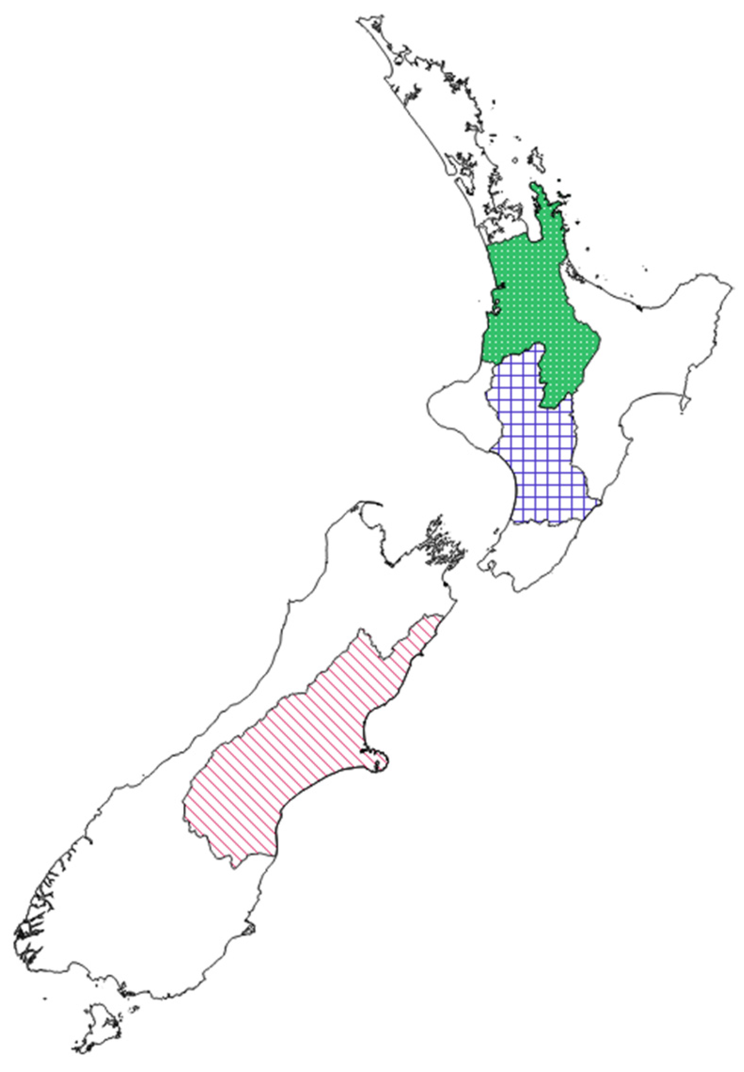
2.1. Location and Farming Details of the Studied Farms

A total of 28 irrigated and 60 non-irrigated ‘rain-fed’ pastoral dairy farms were analysed in different regions of New Zealand.

Table 1. Average characteristics of the pastoral dairy farms (during two years from 2013 to 2015) studied across different regions of New Zealand.

Farm Parameters	Unit	Waikato Non-Irrigated	Waikato Irrigated	Manawatu Non-Irrigated	Manawatu Irrigated	Canterbury Irrigated
Farm count	-	42	3	18	5	20
Average grassland area	ha/farm	172	132	172	363	212
Average stocking rate	Cows/ha	3.16	3.23	2.53	2.35	3.87
Milk production (FPCM) *	L/cow/yr	5224	5796	5052	5339	5263
Electricity use on-farm	kW h/ha/yr	482.5	559.70	482.5	564.98	608.3
Brought-in maize silage	kg DM/ha/yr	1120	1200	1130	1030	1530
Brought-in pasture silage	kg DM/ha/yr	0	0	0	0	1530
Brought-in palm kernel expeller	kg DM/ha/yr	2800	2100	2000	1800	0
Barley grain	kg DM/ha/yr	0	0	0	0	1190
Wheat grain	kg DM/ha/yr	0	0	0	0	1200
Annual rainfall	mm/ha	1053	1074	1030	857	637
Applied irrigation	mm/ha/yr	0	250	0	417	658
Irrigated Area	ha/farm	0	81	0	238	212
% irrigated	%	0	61	0	66	100

Note: * fat- and protein-corrected milk.

summarises average descriptions of the farms involved in this study. The farms were located in three regions with different climatic conditions across New Zealand (Figure 1). The Waikato region is the furthest north, receiving adequate rainfall (>1000 mm yr⁻¹), so pastoral dairy farming in this region is dominated by non-irrigated dairy farms (Table 1). There are some irrigated dairy farms in the region. They do not require irrigation to exist as dairy farms but apply some irrigation to fill soil moisture deficits and increase pasture production over the summer period (from December to March). We selected three irrigated (~396 ha) and 42 non-irrigated (~7224 ha) dairy farms, representing 1.6% of the total dairy ha in the Waikato region.

The Manawatu region is located further south of the Waikato region (Figure 1) and is divided by a mountain range in between. The south-east areas of the Manawatu region receive adequate rainfall (>1000 mm yr⁻¹), where pastoral dairy farms are mainly non-irrigated ‘rain-fed’. The south-west area of the Manawatu region receives relatively low rainfall (<1000 mm yr⁻¹), where the irrigated pastoral dairy farms are mainly located. We selected five irrigated (~1815 ha) and 18 non-irrigated (~3096 ha) dairy farms, representing 4.1% of the total dairy ha in the Manawatu region. The irrigated farms in the Manawatu region are mainly located on sandy coastal soils and operate with lower stocking rates than farms in the rest of the region (Table 1). The Canterbury region is the furthest south of the farms investigated. They lie east of the Southern Alps mountain range in an area of low rainfall (<700 mm yr⁻¹). Pastoral dairy farms in the Canterbury region are mostly irrigated, as the rainfall is insufficient to sustain adequate grass growth year-round. We selected 20 irrigated (~4240 ha) pastoral dairy farms, representing 1.5% of the total dairy ha in the Canterbury region.

The farms’ data were collected from individual farms through a questionnaire. The collated data included records of the grassland area, stocking rates, brought-in feed, and farm milk production for two years from 2013 to 2015 (Table 1).

Figure 2 presents a schematic of the water flows within the farm system boundaries for raw milk production and water use on a pastoral dairy farm platform. In this study, we analysed the water footprints of the studied dairy farms (Table 1), with the scope limited to the direct use of water at the farm and the indirect use of water for imported feed. Water use outside the farm gate, including transport, processing, fertiliser production, and electricity use, was not considered. Water use for the processes excluded here was estimated to be much smaller than direct water use [7]. However, the indirect blue water evaporative losses associated with electricity and fertilisers could be relatively higher than the blue water used directly on non-irrigated dairy farms in the Waikato region [7].

This study specified the function unit as one kilogram of energy-corrected milk, i.e., milk corrected for fat and protein (FPCM). The FPCM (Equation (1)) was calculated using the recorded milk production per day [25,26], as follows:

$$Fat and Protein Corrected Milk (FPCM)=milk per day \left(kg\right)\times \frac{\left[\left(383\times fat \%\right)+\left(242\times protein \%\right)+783.2\right]}{3.14}$$

(1)

The average FPCM was calculated for both the irrigated and non-irrigated farms in each region in further analyses. The estimated water use was divided between milk and meat production using economic allocation criteria [8], with 92% of the water use allocated to milk production and the remainder to meat production [7].

2.2. Water Footprint Methods

Water footprinting methods have been developed to account for green, blue, or grey water types [8,10], where green water is defined as the rainfall water use that is held within the soil profile and used by the plants. Blue water is stored and used from groundwater and surface water resources. Grey water is defined as the volume of water required to assimilate a contaminant load to the accepted (standard) level in receiving water bodies [8]. Water footprint methods also account for direct and indirect water uses for a product or process. Direct water use is the water used directly in producing a product, such as green water from rainfall and blue water from irrigation used to grow pasture or feed crops on pastoral dairy farms. Indirect water use is defined as water used indirectly, like in manufacturing fertiliser and producing the electricity used on the farm.

In this study, the direct water footprint is calculated as the green and blue water (m³) consumed to produce 1 kg of FPCM at the studied irrigated or non-irrigated dairy farms across the study regions (Table 1). The indirect water footprint included the green and blue water consumed in imported feed considered to be produced locally. Further, the consumptive blue water footprint volumes (m³/kg of FPCM) were multiplied with the quantified water scarcity characterisation factors at the regional or catchment level to quantify blue water scarcity footprint indices to produce 1 kg of FPCM at the studied farm types (Table 1).

This study applied two water footprint methods, the WFN-based blue water footprint impact index (WFII_blue) [8] and the available water remaining (AWARE)-characterised water scarcity footprint (WF_AWARE) [14], described as follows.

2.2.1. Quantification of Consumptive Green and Blue Water Footprints

The WFN method accounts for the consumption of green and blue water used to produce a product [8]. The consumptive green water footprint, WF_green (m³/kg of FPCM), of the studied dairy farms was calculated using Equation (2) as follows:

$${WF}_{Green}=\frac{{ET}_{green}}{{Yield}_{FPCM}}$$

(2)

where ET_green is the green water consumption (m³/ha), quantified as the evapotranspiration of the pasture and feed produced on the farm and/or feed imported, and Yield_FPCM is the total kilograms of fat- and protein-corrected milk (kg/ha).

The quantification of the blue water footprint included the estimates of the evapotranspiration (ET_blue) (m³/ha) from irrigation water of the pasture and feed produced on the farm and feed imported. It also included the water used (m³/ha) for stock drinking (SDW) and milking parlour washing (MPW) at the farm. In pastoral-based dairy farms across New Zealand, the SDW and MPW are applied to pastural land as effluent applications, which is ‘consumed’ by pasture at the farm through evapotranspiration (Figure 2). Therefore, the consumptive blue water footprint, WF_blue (m³/kg of FPCM), [8] for the studied dairy farms was calculated using Equation (3) as follows:

$${WF}_{blue}=\frac{\sum {ET}_{blue}+SDW+MPW}{{Yield}_{FPCM}}$$

(3)

2.2.2. Blue Water Footprint Impact Index (WFII_blue)

As per the WFN method [8], the consumptive WF_blue (m³/kg of FPCM) (Equation (3)) was further multiplied by the blue water scarcity (WS_blue) (-), calculating the blue water footprint impact index (WFII_blue) (-), as follows:

$${WFII}_{Blue}={WF}_{blue}\times {WS}_{blue}$$

(4)

where WS_blue is the blue water scarcity, defined as the ratio of the total blue water consumed (∑WF_blue) to the total blue water available (WA_blue) in the geographical region [8], as follows:

$${WS}_{blue}=\frac{\sum {WF}_{blue}}{{WA}_{blue}}$$

(5)

where the WA_blue is defined as the natural runoff (R_nat) minus the environmental water requirements (EWRs) [8], as follows:

$${WA}_{blue}=R_{nat}-EWR$$

(6)

WS_blue becomes 1 when all available blue water has been used, significantly affecting the EWRs in the region [8]. The calculated WFII_blue (Equation (4)) is suggested to differentiate the water scarcity impacts of blue water consumption in the production of a product in areas of differing water resources [8,16,18].

2.2.3. The AWARE Method Water Scarcity Footprint (WF_AWARE)

The AWARE method only accounts for the consumption of blue water and does not assess green water use [14]. This method calculates blue water availability minus demand (AMD_i) as a factor to characterise the blue water consumption of a product or process in a region. The AMD_i is calculated by subtracting the water requirements for human water consumption (HWC) and the environmental water requirement (EWR) from the available water (natural runoff including flow regulation) [14], as follows:

$${AMD}_i=\frac{\left(Availability-HWC-EWR\right)}{Area}$$

(7)

The characterisation factor (CF_AWARE) for a region is then calculated as the inverse of AMD_i normalised by dividing the AMD_worldaverage, as follows:

$${CF}_{AWARE}=\frac{AMDworldaverage}{{AMD}_i}$$

(8)

The CF_AWARE factor is dimensionless, expressed in m³ world eq./m³i, representing a relative value of the environmental impact scope of water consumption in a region [14]. The maximum value of CF_AWARE is suggested to be set at 100, where either water demand is greater than water availability, resulting in AMD_i being a negative value and Equation (8) losing its meaning, or AMD_i < 0.01 × AMD_worldaverage. The minimum value of CF_AWARE is also suggested to be set at 0.1, where AMD_i > 10 × AMD_worldaverage. These constraints result in CF_AWARE ranging from 0.1 to 100 to characterise the blue water consumption volumes based on local water stress conditions [8].

Boulay et al. [14] calculated AMD_i and AMD_worldaverage values using the monthly water data from the WATERGAP model [20] on a 0.5 by 0.5 degree grid at a global scale. However, there was lack of relevant data sets to robustly quantify AMD_i on a monthly basis at the local scale (

Table 2. Summary of global and local data sources used in quantification of water footprints of the studied pastoral dairy farms (Table 1) across different regions of New Zealand.

Parameter	Global Data Source	Local Data Source
Rainfall (P) and reference evapotranspiration (ETo)	CLIMWAT 2.0 for CROPWAT [27].	The National Institute of Weather and Atmosphere Virtual Climate Station Network [28].
Effective rainfall (Peff)	USDA Soil Conservation Service method [29].
Crop coefficients (Kc)	Crop coefficients [30,31].	Crop coefficients [30,31].
Green water consumption (ETgreen)	A minimum of ETc and Peff [8].	A locally developed soil water balance model [32], using local climatic and soil conditions.
Irrigation water consumption (ETblue)	Difference between crop water requirements ETc and ETgreen [8,30].	The minimum of the difference between the locally modelled ETc and ETgreen [32] for pasture growth and maize silage, and the difference between crop water requirements ETc and ETgreen [8,30] for pasture silage, barley grain, and wheat grain.
WF Palm Kernel Expeller (cake)	Based on globally average green water volume used to produce palm kernel expeller [31].	Based on globally average green water volume used to produce palm kernel expeller [31].
Imported crops	Imported crops based on the Waikato and Canterbury regions from 2004 to 2005 [7].	Average farm imports estimated by the modelling team at Dairy NZ (T. Chikazhe; DairyNZ, Hamilton, New Zealand, Pers. Comm. 2016).
Stock drinking water use (SDW)	Estimated stock drinking water [7].	Locally measured stock drinking water [23,24].
Milking parlour water use (MPW)	Estimated milking parlour water use [7].	Locally measured milking parlour water [23,24].
Available water (WA)		A locally calibrated and validated rainfall–runoff model [33].
Environmental Water Requirements (EWRs)		Based on local water allocation limits in the Waikato region. Environmental requirements of 37% were used as suggested for New Zealand [7,34].
Water abstractions (WU)		Locally recorded water allocations and actual water abstraction estimates from Aqualinc [35].
Water consumption (HWC)		Locally estimated actual water abstractions from Aqualinc [35] and consumptive water fraction from Shiklomanov and Rodda [36].
WULCA—CFAWARE	Global layer [19].	Calculated from the locally sourced data listed in this table.
WFN—WSblue	Global layer [18,37].	Calculated from the locally sourced data listed in this table.

). Therefore, in this study, we multiplied the AMD_worldaverage (at 0.0136 m³/m²-month) by 12 to calculate and apply the average annual CF_AWARE factor (Equation (8)) using the available annual water flows in the study regions and catchments.

The water scarcity footprint metric (WF_AWARE), expressed in m³ world eq., was then calculated by multiplying the consumptive WF_blue (m³/kg of FPCM) (Equation (3)) with the corresponding CF_AWARE factor (Equation (8)) for each region, as follows:

$${WF}_{AWARE}={WF}_{Blue}\times {CF}_{AWARE}$$

(9)

The calculated WF_AWARE (Equation (9)) is suggested to differentiate the water scarcity impact of blue water consumption in producing a product in areas of differing water resources [14,16].

2.2.4. Data Sources and Spatial Scale

The data required for applying the above-described two water footprint methods, WFII_blue (Equation (4)) and WF_AWARE (Equation (9)), were collected from different databases, models, and measurement sources, categorised as global or local data sources (Table 2).

The analysis was further carried out considering two different spatial scales, the regional and catchment scales. The regional scale considers the entire region (Figure 1), with many different catchments and water management zones within a similar climatic condition. The catchment or water management zone scale is the hydrological area where all water flows to one major waterway or water body in the area.

The study data collection and analysis were conducted for two (2) years from 1 June 2013 to 31 May 2015 (Table 1). The green and blue water evapotranspiration (ET_green and ET_blue) were quantified for the on-farm pasture production over the entire year and the imported feed over the growing period for the individual crops (Table 1).

Global Data Sources

In the case of global data sources (Table 2), the green water consumption in pasture and feed production was quantified as ET_green, using the average monthly effective precipitation (P_eff) and reference evapotranspiration (ET_o), based on climatic data taken from CLIMWAT 2.0 for CROPWAT [27]. The global CLIMWAT 2.0 database [27] provided the required climatic data from the Hamilton Aerodrome site for the Waikato region, the Palmerston North Aerodrome site for the Manawatu region, and the Christchurch Gardens site for the Canterbury region.

The reference evapotranspiration (ET_o) was multiplied with a crop coefficient (K_c) of 1.05 [29] to calculate the potential evapotranspiration (ET_C) for pasture production in different regions. Effective precipitation was calculated using monthly precipitation (P) collected from CLIMWAT 2.0 [27]. The USDA Soil Conservation Service method [29] was applied over a ten-day time step to quantify precipitation (P_eff), as follows:

$$P_{eff}=P\frac{\left(\frac{125}{3}\right)-0.2\times P}{\left(\frac{125}{3}\right)}for P\le 83.3 \mathrm{mm}/10 \mathrm{days} period$$

(10a)

$$P_{eff}=\left(\frac{125}{3}\right)+0.1 for P>83.3 \mathrm{mm}/10 \mathrm{days} period$$

(10b)

The ET_green for pasture production was then calculated as the minimum of the P_eff and the crop-specific evapotranspiration (ET_c) [8,30], as follows:

$${ET}_{green}={\min [ET}_c,P_{eff}]$$

(11)

The ET_green for imported feed was also calculated over the growing period for the individual crops detailed in Table 1. The ET_green of locally imported pasture silage, maize silage, barley, and wheat was quantified (Equation (11)), assuming their growth under local climatic conditions. The feed crops imported into the Canterbury region were assumed to be grown under irrigation. In contrast, the feed crops imported in the Waikato and Manawatu regions were assumed to be rain-fed grown. The ET_green for each locally produced crop (ryegrass pasture silage, maize silage, wheat, and barley) was calculated (Equation (11)) using the estimates of the average monthly ET₀ and effective precipitation (P_eff) from CLIMWAT 2.0 [27,29]. The crop coefficient (Kc) values for the imported crops (ryegrass pasture silage, maize silage, wheat, and barley) were taken from [30,31]. The irrigation water consumption (ET_blue) was calculated as the deficit between ET_c and ET_green [8,30], as follows:

$${ET}_{blue}=\left({ET}_c-{ET}_{green}\right)$$

(12)

The quantified ET_green and ET_blue for pasture and locally produced feed crops (mm/ha) (Equations (11) and (12)) were then converted to WF_green and WF_blue (L/kg of FPCM) by using the average stocking rate and milk production on the studied farms (Table 1). The total WF_green of feed at the study dairy farms was calculated by summing all the individual green water footprints of imported and farm-grown feed inputs (Table 1). The WF_green of palm kernel expellers (palm kernel cake, PKE) was taken from Chapagain and Hoekstra [31].

The WF_blue was estimated as the total of the irrigation water evapotranspired (ET_blue) and the consumptive fractions of the MPW and SDW used on the farms. The MPW and SDW were calculated from generic industry volumes (70 L/cow per day for MPW; 70 L/cow per day for SDW) for the lactating and non-lactating periods of the year [7]. The SDW and MPW were further corrected as a 78% consumptive ‘evapotranspired’ fraction of the total SDW and MPW used on the farm [36].

Global data sets of the WS_blue and CF_AWARE characterisation factors (Equation (5) and Equation (8), respectively) were downloaded as geographic data layers developed by Mekonnen and Hoekstra [37] and WULCA [19], respectively. The global WS_blue and CF_AWARE data layers were overlaid onto the studied regional and catchment boundaries (Figure 1) to calculate and use the average values of WS_blue and CF_AWARE factors for the characterisation of the quantified WF_blue into WFII_blue (Equation (4)) and WF_AWARE (Equation (9)) indices, respectively, for a kg of FPCM produced at the studied irrigated farms across the study regions and catchments.

Local Data Sources

In the case of local data sources (Table 2), the ET_green and ET_blue were calculated for representative irrigated and non-irrigated conditions at the studied farms (Table 1). A locally developed soil water balance model [32] was applied to quantify ET_green and ET_blue for pasture production at each site. In this model, evapotranspiration (E_t) is quantified as a function of local climatic conditions (potential evapotranspiration, E_t,w) and soil water storage (S), where a and b are locally calibrated constants for a soil type, as follows:

$$E_{t,s}=\left(a+bS\right) and E_t=E_{t,w} if E_{t,w}<E_{t,s}$$

(13)

The soil profile available water values were taken from S-Maps [38], a locally developed soil database (https://smap.landcareresearch.co.nz/; accessed on 1 June 2017). The local climate data were collected from the Virtual Climate Station Network (VCSN) (https://data.niwa.co.nz/#/home; accessed on 1 June 2017). The VCSN takes data from locally observed meteorological stations throughout New Zealand and interpolates the data over a 5 × 5 km grid for all of New Zealand [28].

However, the ET_green and ET_blue for locally produced feed crops (pasture silage, barley grain, and wheat grain), excluding PKE, were calculated as per Equation (11) and Equation (12), respectively, using the local climate data from the VCSN database [28]. In this case, the reference evapotranspiration, ET_o, was calculated using the FAO-56 method [30] and crop coefficient (Kc) values for feed crops (ryegrass pasture silage, maize silage, wheat, and barley) taken from Allen et al. [30] and Chapagain and Hoekstra [31]. In the Canterbury region, it was assumed that all feed grown was irrigated and that the climate was the same as the studied farms. In the Manawatu and Waikato regions, it was assumed that all feed crops were rain-fed and grown in a climate equivalent to the local farms.

The SDW and MPW were calculated from detailed on-farm water meter recordings at the studied farms, except the irrigated dairy farms in the Waikato region [23,24]. The MPW and SDW on the Waikato irrigated dairy farms were not directly measured but calculated from locally developed models by Higham et al. [23,24]. As in the case of the global data, a fraction of 78% (based on Shiklomanov and Rodda [36]) was applied to calculate the consumptive fraction of the SDW and MPW, considering its discharge as an effluent applied to pasture land at NZ pastoral dairy farms.

The locally available hydrological data and models were used to quantify WS_blue (Equation (5)) and CF_AWARE (Equation (8)) factors for the study regions and catchments. The available water (WA) was quantified as the natural runoff (R_nat) using the average rainfall (P) minus actual evapotranspiration (ET), estimated using a locally calibrated and validated model from 1960 to 2006 [33]. The total water consumption (HWC) was calculated from the recorded average annual water allocations and estimates of actual water abstraction and fractions consumed in the study regions and catchments. In New Zealand, the Regional Councils require consent for water abstraction for public water supply and industrial and agricultural water use in their regions [39]. Regional Councils supplied the total consented water for different purposes (drinking, industrial, and agricultural) in the study regions and catchments during the study years (2013–15). Based on the locally published data and information available [35,39], the water abstraction (withdrawal) rates of the allocated water locally were estimated at 55% for the Canterbury region, 28% for the Manawatu region, and 38% for the Waikato region. Estimates of actual water consumption fractions for agriculture (0.78), industrial use (0.10), and public supply (0.13) were used to calculate the amounts of water consumed from the estimated water abstraction [36]. Any local records of water transfers for hydroelectricity generation to and from the study regions were collected directly from the power companies. These water transfers were considered a net gain of available water for the receiving region and a consumptive take in the region losing the water.

The quantification of WS_blue (Equation (5)) and AMD_i (Equation (7)) also requires estimates of environmental water requirements (EWRs) in a region. However, there are different methods and considerable ranges in EWR estimation [7,8,14,40]. Therefore, we used a range of EWRs for the WS_blue and AMD_i methods to analyse their effect on the resulting blue water footprint impact indices, WFII_blue and WF_AWARE, for pastoral dairy milk production in the study regions and catchments. The EWR rates were set at 37% of the mean annual runoff (MAR) following Zonderland-Thomassen and Ledgard [7]; 30% and 60% of the MAR as the minimum and maximum range, as suggested by Pastor et al. [40]; 80% of the MAR, as suggested by [8]; and a locally estimated EWR for water flow regulations in the Waikato region, where 10% of the Q5 (5-year, 7-day, low flow rate) can be allocated for EWRs, equating to 64% of the MAR in the Karapiro catchment in the Waikato region.

3. Results

3.1. Consumptive Water Footprint and Its Variation on the Studied Pastoral Dairy Farms

Table 3. Consumptive water footprints (L/kg of FPCM ¹) of the studied pastoral dairy farms across different regions of New Zealand.

Water Consumed (L/kg of FPCM 1)	Global Data					Local Data
	Irrigated Farms			Non-Irrigated Farms		Irrigated Farms			Non-Irrigated Farms
	Canterbury	Manawatu	Waikato	Manawatu	Waikato	Canterbury	Manawatu	Waikato	Manawatu	Waikato
SDW 2	2.7	2.1	1.2	2.7	2.7	1.2	1.9	2	2.1	2.2
MPW 2	2.4	3.8	2.9	2.4	2.4	3.2	2.5	2.2	2.6	2.4
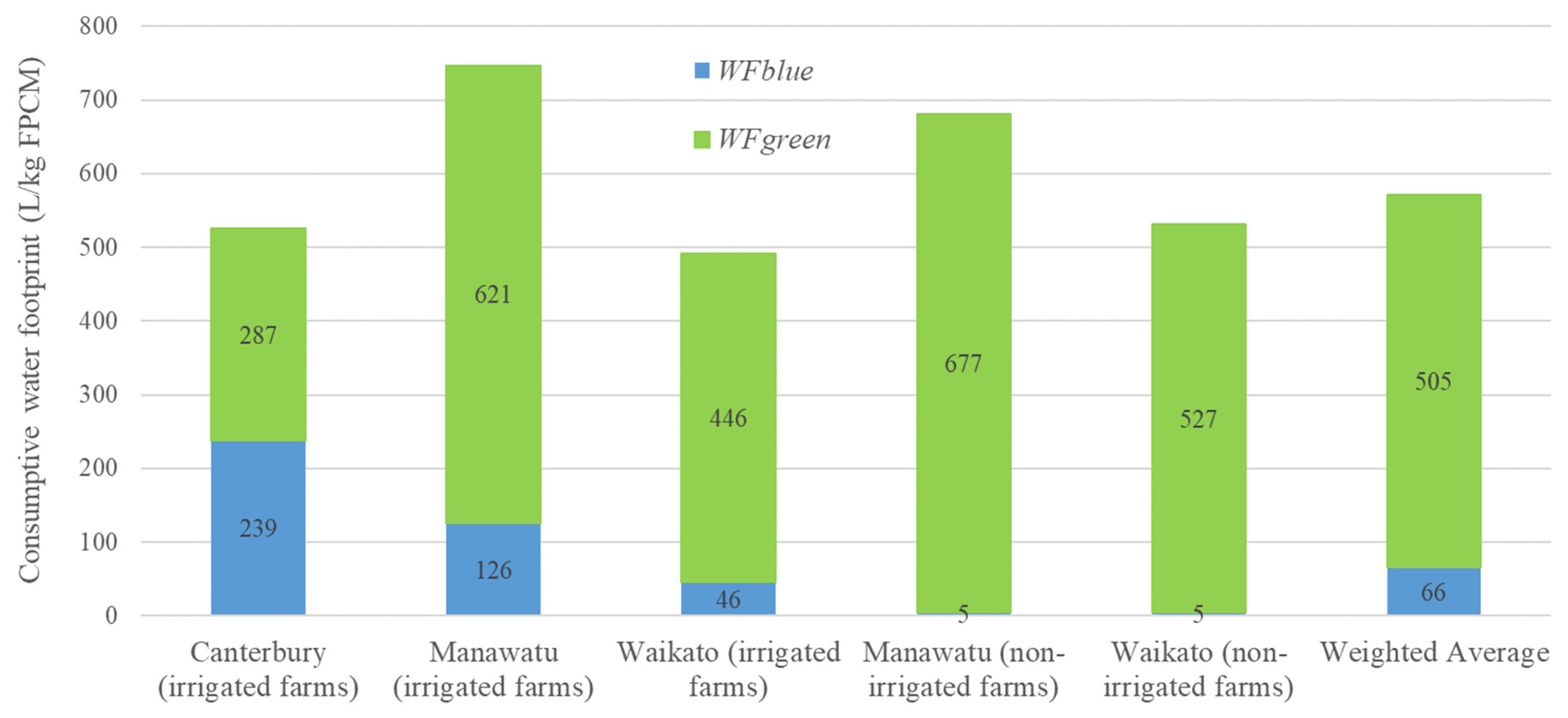
ETgreen	253	546	371	535	371	287	621	446	677	527
ETblue	240	181	107	0	0	234	122	42	0	0
WFblue	246	187	111	5	5	239	126	46	5	5
WFgreen	253	546	371	535	371	287	621	446	677	527
Total WF	499	733	482	540	376	525	747	492	682	531

Notes: ¹ L/kg of FPCM = litres of water used to produce 1 kg of fat- and protein-corrected milk. ² SDW = stock drinking water, MPW = milking parlour water use.

summarizes the consumptive green and blue water footprints (expressed in litres of water per kg of FPCM) of the studied farms, calculated using global and local data sources (Table 2). About 99% of the total consumptive WF was quantified as being associated with water consumption via evapotranspiration (ET) for pasture and feed production at the studied farms. However, the consumptive ET_green and ET_blue for pasture and feed production at the studied farms varied considerably depending on their location and whether they were non-irrigated (rain-fed) or irrigated (Table 3).

The studied dairy farms in the Manawatu region were assessed to have a higher consumptive WF than the studied farms in both the Waikato and Canterbury regions. The consumptive WF_green (L/kg of FPCM) in the Manawatu region was estimated to be about 22 to 54% higher than in the Waikato and Canterbury regions (Table 3; local data). A relatively higher WF_green in the Manawatu region is partly explained by the differences in the potential evapotranspiration rates and stocking rates, leading to lower production per hectare and higher rainfall water consumed per kg of FPCM in the Manawatu region.

The irrigated dairy farms in the Manawatu and Waikato regions resulted in no significant differences in their total consumptive WF (L/kg of FPCM) compared to the non-irrigated dairy farms in the regions (Table 3; local data). Less irrigation is required in the Manawatu and Waikato regions, which receive relatively higher rainfall (>850 mm per year), especially in the Waikato region (Table 3; local data). The ET_blue was estimated, on average, to be only 9 to 16% of the total ET (i.e., ET_green plus ET_blue) at the studied farms in the Waikato and Manawatu regions (Table 3; local data). However, the ET_blue was estimated to be as high as 45% of the total ET at the studied farms in the Canterbury region. As a result, the consumptive WF_blue (L/kg of FPCM) of the studied irrigated dairy farms in the Canterbury region was estimated to be about two to five times higher compared to the studied irrigated dairy farms in the Manawatu and Waikato regions, respectively (Table 3; local data). This is because of relatively low rainfall (<650 mm per year), hence the higher irrigation water use on pastoral dairy farms in the Canterbury region (Table 1).

3.2. Effect of Water Footprint Methods

The consumptive water footprints are suggested to be characterised using local water stress or scarcity indices to assess their environmental water scarcity impacts in the study regions [8,14,15,16].

Table 4. Water scarcity footprint characterization factors (CFs), the blue water scarcity index (W_Sblue) and the blue water availability minus demand (CF_AWARE), calculated for the study regions in New Zealand. Note relative ranks shown in parentheses (1 representing the lowest value).

Region	Global Data		Local Data
	WSblue (-)	CFAWARE (m3 World eq./m3)	WSblue (-)	CFAWARE (m3 World eq./m3)
Waikato	0.002 (1)	0.765 (1)	0.014 (1)	0.300 (1)
Manawatu	0.010 (2)	0.895 (2)	0.098 (2)	0.403 (2)
Canterbury	0.371 (3)	7.355 (3)	0.190 (3)	0.473 (3)
Range (min.–max.)	0.002–0.371	0.765–7.355	0.014–0.190	0.300–0.473

and

Table 5. Characterization factors (CFs), the blue water scarcity index (W_Sblue) and the blue water availability minus demand (CF_AWARE), calculated for the study catchment or water management zones in New Zealand. Note relative ranks shown in parentheses (1 representing the lowest value).

Region: Catchment/ Water Management Zone	Global Data		Local Data
	WSblue (-)	CFAWARE (m3 World eq./m3)	WSblue (-)	CFAWARE (m3 World eq./m3)
Waikato region
Waikato River	0.002 (1)	0.612 (2)	0.031 (1)	0.314 (2)
Waihou	0.006 (2)	0.600 (1)	0.032 (2)	0.307 (1)
Manawatu region
Rangitikei River	0.008 (3)	1.074 (3)	0.257 (4)	0.564 (5)
Canterbury region
Orari-Opihi-Pareora	0.673 (6)	40.840 (6)	0.129 (3)	0.874 (6)
Selwyn-Waihora	0.353 (5)	2.371 (4)	0.361 (5)	0.484 (3)
Ashburton	0.234 (4)	3.025 (5)	0.375 (6)	0.502 (4)
Range (min.–max.)	0.002–0.673	0.600–40.840	0.031–0.375	0.0.314–0.874

present values of the characterisation factors, the WS_blue (Equation (5)) [8] and the CF_AWARE (Equation (8)) [14], calculated using global and local data sources (Table 2) at the regional scale (Table 4) and catchment/water management zone scale (Table 5).

The CF_AWARE yielded relatively higher absolute values than the WS_blue (Table 4 and Table 5). This was expected due to accounting for different water variables and formulations used in the quantification of WS_blue (Equation (5)) and CF_AWARE (Equation (8)). The WS_blue quantifies the ratio of the cumulative consumptive water footprint (∑WF_blue) to the total blue water availability (WA) minus environmental flow requirements (EWRs) in a geographical area (Equation (5)). The CF_AWARE also accounts for total human water consumption (HWC) (equivalent to the ∑WF_blue), WA, and EWRs in a geographical area. However, the CF_AWARE quantifies the available water remaining (AMD_i) per unit area (Equation (7)) and further normalises the CF_AWARE by dividing the AMD_worldaverage by the calculated AMD_i for the study area (Equation (8)) [14].

Despite the differences in their formulations, both water footprint methods, interestingly, ranked different study regions in the same order (from lowest to highest) in terms of blue water scarcity (WS_blue) or the blue water availability minus demand (CF_AWARE) (Table 4). However, this consistency in the relative ranking order of the WS_blue and CF_AWARE factors was somewhat limited at the catchment or water management zone scale (Table 5). This slight inconsistency in the relative ranking order of the WS_blue and CF_AWARE factors at the catchment or water management zone scale (Table 5) was also reflected in the quantification and relative rankings of the blue water scarcity impact index (WFII_blue) (Equation (4)) and the water scarcity footprint metric (WF_AWARE) (Equation (9)) for a kg of FPCM produced at the studied irrigated farms located in different catchment or water management zones (

Table 6. Quantified water scarcity footprint metrics, the blue water footprint impact index (WFII_blue) and the Available WAter REmaining-characterised water scarcity footprint (WF_AWARE), for pastoral dairy milk production (per kg of FPCM) at the studied irrigated dairy farms in the study catchment and water management zones in New Zealand. Note relative ranks shown in parentheses (1 representing the lowest value).

Region: Catchment/ Water Management Zone	Global Data		Local Data
	WFIIblue (-)	WFAWARE (m3 World eq./kg of FPCM)	WFIIblue (-)	WFAWARE (m3 World eq./kg of FPCM)
Waikato region 1	0.20	92.65	0.63	13.86
Waikato River	0.21 (1)	68.16 (2)	1.44 (1)	14.48 (2)
Waihou	0.66 (2)	66.84 (1)	1.46 (2)	14.16 (1)
Manawatu region 1	1.95	181.57	12.39	50.88
Rangitikei River	1.48 (3)	200.45 (3)	32.49 (4)	71.31 (3)
Canterbury region 1	99.09	1962.67	45.41	112.80
Orari-Opihi-Pareora	165.31 (6)	10,026.24 (6)	30.84 (3)	208.39 (6)
Selwyn—Waihora	86.63 (5)	581.97 (4)	86.03 (5)	115.39 (4)
Ashburton	57.46 (4)	742.75 (5)	89.52 (6)	119.69 (5)
Range (min.–max.)	0.21–165.31	68.16–10,026.24	1.44–89.52	14.48–208.39

Notes: ¹ The average values for all the study farms in the region.

). Also, in absolute value terms, the AWARE-based WF_AWARE values were quantified higher than the WFN-based WFII_blue values, especially using global data sources (Table 6).

Overall, however, both water scarcity footprint indices, WFII_blue and WF_AWARE, ranked the study regions or catchments/water management zones in a similar order (lowest to highest) based on the quantified water scarcity footprint for a kg of FPCM produced at the studied irrigated dairy farms across the study regions and catchments (Table 6).

3.3. Effect of Local and Global Data Sources

Compared to the local data sources, using global data sources (Table 2) resulted in over- and underestimation of the consumptive WF of dairy milk production at different farm types (irrigated or non-irrigated) in the study regions (Table 3). The use of global data sets resulted in an overestimation of the SDW (in terms of L per kg of FCPM) by 125% for the studied irrigated farms in the Canterbury region and by 23 to 29% for the studied non-irrigated farms in the Waikato and Manawatu Regions. However, using global data sets resulted in an underestimation of 40% in the SDW for the studied irrigated farms in the Waikato region. The use of global data sets also underestimated the MPW by 25% for the studied irrigated farms in the Canterbury region and 8% for the studied non-irrigated farms in the Manawatu Region. In contrast, the global data sets overestimated the MPW by 52 and 32% for the studied irrigated farms in the Manawatu and Waikato regions, respectively (Table 3).

The ET_green for pasture and feed production based on the globally available CLIMWAT database (Table 2) was underestimated by 12 to 30% on all studied farms compared to the estimates based on the locally available climatic database, the VCSN [28]. In contrast, the global CLIMWAT data-based ET_blue was overestimated, particularly in the Manawatu and Waikato regions. The global CLIMWAT data-based ET_blue was estimated about 48 and 155% higher for the studied irrigated farms in the Manawatu and Waikato regions, respectively. These differences in the estimation of the ET_green and ET_blue for pasture and feed production could be mainly attributed to the estimates of less effective rainfall in the global data sets compared to the local data set. Therefore, the irrigation requirements were estimated to be relatively higher using the global CLIMWAT data set [27] than the local climatic data set [28]. Overall, the use of global data sets in this study resulted in the total consumptive WF (green plus blue water) being underestimated by 2 to 5% for the irrigated farms and 21 to 29% for the non-irrigated farms (Table 3).

Compared to the local data sources, using global data sources (Table 2) also affected the quantification of the water scarcity characterisation factors, WS_blue (Equation (5)) and CF_AWARE (Equation (8)), at the regional and catchment scales (Table 4 and Table 5). The CF_AWARE based on the global WULCA data layer [19] was estimated at 7.355 for the Canterbury region, which was about 16 times higher compared to the CF_AWARE value of 0.473 estimated by using local data (Table 4). The global CF_AWARE layer, as compared to the locally calculated CF_AWARE values, also resulted in CF_AWARE values that were >two times higher for the Manawatu and Waikato regions (Table 4). The global WS_blue layer [37], as compared to the locally calculated WS_blue values, resulted in 95% higher WS_blue values for the Canterbury region but 86 and 90% lower WS_blue values for the Waikato and Manawatu regions, respectively (Table 4). The global data layers resulted in a slightly higher range in the WS_blue and CF_AWARE values for the study regions (Table 4). However, interestingly, using either global or local data, the study regions were ranked in a similar order (from lowest to highest) in terms of the WS_blue and CF_AWARE values (Table 4), showing the lowest water stress in the Waikato region and the highest in the Canterbury region.

The WS_blue and CF_AWARE values were also under- or overestimated when using the global data layers at the catchment scale (Table 5). Compared to the local data estimates, the global WULCA data layer [16] reported the CF_AWARE as being 47 times higher for the Orari-Opihi-Pareora water management zone (Table 5). This zone had a higher global CF_AWARE value assigned because the pixel on which it was calculated resided over the area of greater water use in the zone, not the area in the zone where most of the available water is generated in the headwaters. However, the WS_blue values were estimated relatively lower in the global data set [37], except for the Orari-Opihi-Pareora water management zone (Table 5).

The use of different data sources had a significant effect on the overall quantification of the water scarcity footprint indices, the WFN-based WFII_blue (-) (Equation (4)) and the AWARE-based WF_AWARE (m³ world eq./kg of FPCM) (Equation (9)), for the pastoral dairy milk production across the study catchments (Table 6). As compared to the local data estimates, the global data sets (Table 2) resulted in the quantification of the WFII_blue (-) being 36 to 95% lower for most of the study catchments, except Orari-Opihi-Pareora and Ashburton in the Canterbury region (Table 6). In contrast, the global data sets (Table 2) resulted in the quantification of the WF_AWARE (m³ world eq./kg of FPCM) being 3 to 47 times higher for the study catchments, notably 47 times higher for Orari-Opihi-Pareora in the Canterbury region (Table 6). The higher WF_AWARE values based on the global data (Table 6) could be attributed to the relatively higher CF_AWARE values quantified by the global WULCA data layer [16] for the study catchments (Table 5).

Table 7. Sensitivity of the water scarcity footprint characterization factors (CFs) and characterised water scarcity footprint indices for pastoral milk production on the studied irrigated dairy farms to different environmental water requirements (EWRs) in different regions of New Zealand.

Water Footprint Method	EWR 1	Water Scarcity Characterization Factors			Water Scarcity Footprint Indices
		Waikato	Manawatu	Canterbury	Waikato	Manawatu	Canterbury
WFN-based method [8]		WSblue (-)			WFIIblue (-)
	0.30	0.01	0.09	0.17	0.57	11.15	40.87
	0.37	0.01	0.10	0.19	0.63	12.39	45.41
	0.60	0.02	0.15	0.30	0.95	19.51	71.51
	0.64	0.02	0.17	0.34	1.05	21.89	80.26
	0.80	0.04	0.31	0.60	1.72	39.01	143.03
AWARE method [12,14]		CFAWARE (m3 world eq./m3)			WFAWARE (m3 world eq./kg of FPCM)
	0.30	0.27	0.36	0.42	12.54	45.30	99.19
	0.37	0.30	0.40	0.47	13.86	50.88	112.80
	0.60	0.46	0.82	0.86	21.14	103.23	205.44
	0.64	0.51	0.97	1.02	23.48	122.27	243.33
	0.80	0.84	1.68	3.01	38.95	212.20	718.84

Note: ¹ Percentage of mean annual runoff required for the environmental water requirements.

presents a further evaluation of the effects of local data in terms of different EWRs on the quantification of the WFII_blue (-) (Equation (4)) and the WF_AWARE (m³ world eq./kg of FPCM) (Equation (9)) values for the studied irrigated farms in the study regions. Depending on the EWR rates used (30 to 80% of the mean annual runoff (MAR)), the quantified WFII_blue (-) varied by a factor of 3 to 3.5 times in the study regions (Table 7). Similarly, the quantified WF_AWARE (m³ world eq./kg of FPCM) varied by a factor of 3 to 7.2 times in the study region (Table 7). Table 7 highlights a very high sensitivity of the quantification of the WFII_blue and WF_AWARE values based on the set EWR rates used in the study regions.

3.4. Effect of Spatial Scale

The effect of different spatial scales of analysis can be seen in Figure 3, which presents the consumptive WF (L/kg of FCPM) quantified using the local data sets (Table 2) for the studied irrigated and non-irrigated dairy farms in the study regions (Table 1). The consumptive WF_green varied from 287 L per kg of FCPM for the studied irrigated farms in the Canterbury region to 677 L per kg of FCPM for the studied non-irrigated farms in the Manawatu region, with a weighted average of 505 L per kg of FCPM for all studied irrigated and non-irrigated farms across all study regions (Figure 3).

Compared to the weighted average, the WF_green was quantified as being 43% lower for the studied irrigated farms in the Canterbury region but 34% higher for the studied non-irrigated farms in the Manawatu region. In contrast, as compared to the weighted average, the consumptive WF_blue was quantified >260% more for the studied irrigated farms in the Canterbury region but about 90% less for the studied non-irrigated farms in the Manawatu and Waikato regions (Figure 3 and Table 3).

Table 6 also further demonstrates the effect of different spatial scales of analysis on the characterised blue water scarcity footprint indices, the WFII_blue (-) and the WF_AWARE (m³ world eq./kg of FPCM), for the studied irrigated farms in different regions and catchments/water management zones. Using the local data sets, the quantified WFII_blue varied from 1.44 (-) per kg of FPCM in the Waikato River catchment to 89.52 (-) per kg of FPCM for the studied irrigated dairy farms in the Ashburton water management zone (Table 6). The WFII_blue values were quantified 89 to 97% higher for Selwyn-Waihora and Ashburton but −32% lower for Orari-Opihi-Pareora than the rationalised WFII_blue value of 45.41 (-) for the Canterbury region. Similarly, the quantified WF_AWARE varied from 14.16 m³ world eq./kg of FPCM for the study irrigated dairy farms in the Waihou catchment to 208.39 m³ world eq./kg of FPCM for the study irrigated dairy farms in the Orari-Opihi-Pareora water management zone. The WF_AWARE values were quantified only 2 to 6% higher for Selwyn-Waihora and Ashburton than the rationalised WF_AWARE value of 112.80 m³ world eq./kg of FPCM for the Canterbury region (Table 6). In contrast, the WF_AWARE value for the Orari-Opihi-Pareora water management zone was quantified 85% higher than the rationalised WF_AWARE value of 112.80 m³ world eq./kg of FPCM for the Canterbury region. Also, the WF_AWARE value for the studied irrigated farms in the Rangitikei River catchment was quantified about 40% higher than the rationalised WF_AWARE value of 50.88 m³ world eq./kg of FPCM for all studied irrigated farms in the Manawatu region (Table 6).

4. Discussion

4.1. Evaluation of Water Footprint Methods

Water footprinting methods are under development for their potential applications for a robust assessment of water scarcity impacts associated with agricultural production, including pastoral dairy farming. In this study, the two water scarcity footprint indices, the WFN-based WFII_blue [8] and the AWARE-based WF_AWARE [14], resulted in different absolute values of the water scarcity footprint associated with a kg of FPCM (Table 6) produced at the studied irrigated and non-irrigated pastoral dairy farms in different regions of New Zealand (Table 1). This is expected due to the different formulations used for the quantification of the WFII_blue (Equation (5)) and WF_AWARE (Equation (9)). However, interestingly, the quantified WFII_blue and WF_AWARE values ranked the study regions and catchments in a similar order of lowest to the highest magnitude in terms of the water scarcity footprint associated with a kg of FPCM produced (Table 6).

As an exception, the quantified WFII_blue and WF_AWARE values ranked the Orari-Opihi-Pareora water management zone as third and sixth (from lowest (first) to highest (sixth)), respectively (Table 6). This was attributed mainly to differences in the quantification of the relatively higher CF_AWARE for the Orari-Opihi-Pareora water management zone (Table 5). The calculation of the CF_AWARE (Equation (7)) divides the remaining available water (i.e., available water minus human water consumption minus environmental flow requirement) by the geographical area. The Canterbury management zones are quite large in their area and generate their main volumes of water supply mainly in the mountains through snow melt. Including the catchment area in Equation (7) could result in a relatively lower AMD_i value, translating into a relatively higher CF_AWARE (Equation (8)) value for a larger catchment than a smaller one with similar water availability and demands. In contrast, the WSI_blue (Equation (5)) is calculated as a ratio of the cumulative blue water consumption to the total water availability, accounting for environmental water requirements in the geographical area. Using the local data, the WSI_blue was quantified relatively less for the Orari-Opihi-Pareora water management zone (Table 5).

The WFN-based WFII_blue [8] and the AWARE-based WF_AWARE [14] are also highly sensitive to the values of the environmental water requirements used in their calculations (Equations (6) and (7), and Table 7). The WFN-based WFII_blue [8] considers EWRs at a conservative rate of 80% of the mean annual runoff (MAR) [8,37]. The AWARE-based WF_AWARE [14] considers the EWRs calculated using the method of Pastor et al. [40], using the monthly water flows given in the WaterGAP database [20]. The differences in the EWR rates affect the available water and the quantification of water scarcity levels in the study area. Both the WFN-based WFII_blue [8] and the AWARE-based WF_AWARE [14] methods provide adequate means to assess water scarcity using the locally determined EWRs in the study area. However, the AWARE-based WF_AWARE [14] normalises the locally determined water availability minus demand (AMD_i) with the global average (AMD_worldaverage) (Equation (7)) in the calculation of water scarcity levels (CF_AWARE) for a study area (Equation (8)). The normalisation of the locally determined AMD_i with the global average AMD_worldaverage may be helpful when comparing water usage for a product from two different regions. However, it is potentially subjected to uncertainty in terms of the data used to quantify the global average AMD_worldaverage, using global data sources and models [20]. The WFN-based WFII_blue [8] quantifies a water scarcity footprint index that more closely reflects the quantitative volumes of water available and consumed locally in a study area.

However, both water footprint methods, the WFN-based WFII_blue [8] and the AWARE-based WF_AWARE [14], appear to be capable of capturing relative differences in the quantification of the water scarcity footprint indices of a product, e.g., the water scarcity footprint indices for a kg of FPCM analysed in this study.

4.2. Appropriate Data Sources and Spatial Scales

The FAO LEAP guidelines recommend using primary data to assess water use in livestock production systems and supply chains [15,16]. However, considering the challenges and resources required for primary data collection, the modelled data with inputs from secondary data sources are often used to assess water use in livestock production systems [17]. In this study, the use of local and global data sources (Table 2) had a significant impact on the quantification of the consumptive water footprints (Table 3); the water scarcity characterisation factors, the WS_blue (-) and the CF_AWARE (m³ world eq./m³) (Table 4 and Table 5); and the water scarcity footprint indices, the WFII_blue (-) and the WF_AWARE (m³ world eq./kg of FPCM) values for the studied irrigated farms across the study regions and catchments.

Compared to the local data, the use of global data sources resulted in an underestimation of the consumptive WF_green (L/kg of FPCM) by −12 to −30% and an overestimation of the consumptive WF_blue (L/kg of FPCM) by 3 to 141% in the study regions. Hess [41] also found similar effects of an underestimation of annual ET_green calculated using the FAO CROPWAT model with the USDA effective rainfall estimation, as compared to the ET_green simulated with a water balance model using long-term daily or average monthly weather data for the quantification of the water footprint of pasture production in England. Zhuo et al. [42] also reported a higher sensitivity of crop water footprints to climactic inputs of reference evapotranspiration (ET₀) and precipitation (P) in the Yellow River Basin, China. The use of global or local data sets also affected the relative rankings (from lowest to highest) of the water scarcity characterisation factors (WS_blue and CF_AWARE) (Table 5) and the characterised water scarcity footprint indices (WFII_blue and the WF_AWARE) (Table 6) quantified for a kg of FPCM produced on the studied irrigated and non-irrigated pastoral dairy farms. The quantified differences in CF_AWARE and WS_blue values for the study regions and catchments (Table 4 and Table 5) could be attributed to different sources of hydrological and water use data and models used at the global and local levels (Table 2).

The catchment scale is a more appropriate level to quantify water footprints for the assessment of the appropriation of water resources and the environmental impacts of water consumption on local freshwater environments. Water footprint hotspots can be hidden at the regional scale, but they can be seen when analysed at the catchment scale (Table 4 and Table 5). For example, the Selwyn-Waihora and Ashburton water management zones had similar water scarcity values (CF_AWARE and WS_blue) (Table 5). However, Orari-Opihi-Pareora had about 1.85 times higher CF_AWARE and WS_blue values than the regionalised CF_AWARE and WS_blue values for the Canterbury region (Table 4 and Table 5). This example highlights the influences of differences in water availability and use between different catchments on quantifying the water scarcity footprint associated with pastoral milk production across New Zealand.

A majority (~99%) of the consumptive water footprints of a unit of pastoral dairy milk production (L/kg of FPCM) was quantified as being associated with the green and blue water consumption via evapotranspiration for pasture and feed used at the studied dairy farms. The most critical data to collect at the catchment scale are the local climate data and irrigation water use in pasture and feed production for dairy farms. Effective rainfall and evapotranspiration (ET) can be highly variable within a region. The use of global data sources with monthly average climatic data from one location within a region can lead to inaccurate estimates of green and blue consumptive water footprints in a catchment (Table 3) [41,42].

The direct water use on a dairy farm is also important data to quantify accurate water footprints of dairy milk production. The actual irrigation water used, as opposed to water allocated, is also crucial to collect, as if the water is not used, then there is no impact from it being allocated. Compared to the actual measurements (Table 2), the use of globally estimated rates (Table 2) resulted in an over- or underestimation of SDW and MPW on the studied farms (Table 3). While SDW and MPW made up small proportions of the blue water use at the studied irrigated farms, they primarily used blue water at non-irrigated farms for pastoral dairy production (Table 3).

Compared to the local data, the use of global data sources (Table 2) also affected the over- or underestimation of the water scarcity characterisation factors (WS_blue and CF_AWARE) (Table 5) for the study regions and catchments. The global WS_blue and CF_AWARE data layers are mainly based on estimates of coarse-resolution global hydrological models and databases [16,37]. They could be less accurate for regional- and catchment-scale analysis than those calculated using local data (Table 5). The global data layers are divided into pixels (30′ by 30′ for WS_blue, 0.5 by 0.5 degrees for CF_AWARE), which did not align with the studied regional or catchment areas. In the global CF_AWARE layer [16], the pixel covered the lower plains of the Orari-Opihi-Pareora water management zone, where most irrigation occurs. However, it did not include the mountain ranges at the top of the catchment, where most available water is generated. The global WS_blue layer [37] also did not fit very well with the shape of the regions across New Zealand.

One of the main differences in the quantification of the WS_blue and CF_AWARE for the Rangitikei River catchment was the change in their comparative ranking between the use of global and local data sets (Table 5). The WS_blue and CF_AWARE values for the Rangitikei River catchment were ranked third (from lowest (first) to highest (sixth)) in the global data, but ranked fourth or fifth highest, respectively, in the local data set (Table 5). This could partly be due to water transfers between the regions through hydroelectricity schemes from the Rangitikei River into the Waikato River. Therefore, these data are commercially sensitive and not readily available, so they may not be included in the global data sets. However, these data are critical locally to calculate water footprints with, as they can significantly affect the quantification of water scarcity footprints at the local scale.

As presented in Table 7, the use of different environmental water requirements resulted in a high variation in the WFII_blue and WF_AWARE values associated per kg of FPCM produced on the studied irrigated farms across the study regions. Different EWR rates are suggested in the literature for waterways to maintain freshwater ecosystems’ health. They include ranges from 30% and 60% of the mean annual runoff (MAR) as the minimum and maximum range as suggested by Pastor et al. [40]; the conservative value of 80% MAR proposed by the Water Footprint Network [8]; and the 37% MAR already used in other analyses across New Zealand [7]. Suppose that EWRs are calculated using global databases and models compared to the locally determined EWRs. In that case, this may result in a different EWR rate and, therefore, different values of the WFN-based WS_blue and WFII_blue [8] and the AWARE-based CF_AWARE and WF_AWARE [14] indices for a product produced in a catchment. Therefore, the water footprinting methods would benefit from further research and discussion on the appropriate setting of EWR rates, mainly if the quantified water scarcity footprint indices are used for a comparative analysis of different products produced in different catchments.

Also, due to a lack of relevant data availability in this study, it was impossible to quantify the water scarcity characterisation factors (WS_blue and CF_AWARE) on a seasonal or monthly basis to capture better effects of temporal variability in water availability, water consumed, and environmental flow requirements. Therefore, it is critical to develop robust monitoring and modelling tools to quantify water flows, allocations, and uses for different activities in local catchments. This information is critical to robustly quantify and assess water productivity and water scarcity impact footprints to help develop productive and environmentally sustainable food production systems, including pastoral dairy milk production.

5. Conclusions

The consumptive water footprint of a unit of pastoral dairy milk production (L/kg of FPCM) was quantified as being mainly associated (~99%) with green and blue water consumption via evapotranspiration for the pasture and feed used at the studied dairy farms. However, the consumptive green and blue water footprints for pasture and feed varied considerably depending on the farm type (non-irrigated (rain-fed) or irrigated) and their location in different climatic conditions. The consumptive blue water footprint (L/kg of FPCM) of the studied irrigated farms in the Canterbury region was estimated to be about two to five times higher compared to the Manawatu and Waikato regions, respectively, due to relatively low rainfall (<650 mm per year), hence the higher irrigation water use.

The WFN-based blue water footprint impact index (WFII_blue) and the Available WAter REmaining-characterised water scarcity footprint (WF_AWARE) indices are capable of capturing relative differences in quantifying the water scarcity footprint for a kg of FPCM produced on the irrigated farms in the studied regions and catchments. Interestingly, the quantified WFII_blue and WF_AWARE values ranked the study regions and catchments in a similar order of lowest to highest magnitude in terms of the water scarcity levels and the water scarcity footprint values for a kg of FPCM produced.

However, using local or global data sources greatly affected the quantification of the consumptive ‘volumetric’ and the water scarcity footprint indices (WFII_blue and WF_AWARE) associated with a unit of milk production (kg of FPCM) produced. Compared to the local data, the use of global data sources resulted in an underestimation of the consumptive green water footprint (L/kg of FPCM) by −12 to −30% and an overestimation of the consumptive blue water footprint (L/kg of FPCM) by 3 to 141% in the studied regions. The global data sources also resulted in an under- or overestimation of the WFII_blue and the WF_AWARE values, especially the WF_AWARE (m³ world eq./kg of FPCM), which was quantified as being 47 times higher for Orari-Opihi-Pareora in the Canterbury region.

Observations of local climatic data, actual irrigation water use, locally calibrated hydrological models, and environmental flow requirements are critical for accurately quantifying and assessing the water scarcity footprints associated with pastoral dairy milk production in local catchments. The catchment or water management spatial scale should be used for the analysis. Catchments within regions can have varying levels of water availability and water use, which are masked when using a regional or national level of water scarcity characterisation factors in the quantification of water scarcity footprint indices associated with a unit of milk production (kg of FPCM) produced in local catchments. The lack of relevant data availability locally needs to be addressed to robustly quantify the water scarcity characterisation factors (WS_blue and CF_AWARE) on a seasonal or monthly basis to capture better effects of temporal variability in water availability, water consumed, and environmental flow requirements for the quantification of the water scarcity footprint indices (WFII_blue and WF_AWARE) associated with primary production systems, including pastoral dairy milk production in local catchments.

References

- Ridoutt, B.G.; Williams, S.R.O.; Baud, S.; Fraval, S.; Marks, N. The water footprint of dairy products: Case study involving skim milk powder. J. Dairy Sci. 2010, 93, 5114–5117. [Google Scholar] [CrossRef] [PubMed]
- Cosentino, C.; Adduci, F.; Musto, M.; Paolino, R.; Freschi, P.; Pecora, G.; D’Adamo, C.; Valentini, V. Low vs. high “water footprint assessment” diet in milk production: A comparison between triticale and corn silage based diets. Emir. J. Food Agric. 2015, 27, 312–317. [Google Scholar] [CrossRef]
- Palhares, J.C.P.; Pezzopane, J.R.M. Water footprint accounting and scarcity indicators of conventional and organic dairy production systems. J. Clean. Prod. 2015, 93, 299–307. [Google Scholar] [CrossRef]
- Dalla Riva, A.; Burek, J.; Kim, D.; Thomas, G.; Cassandro, M.; De Marchi, M. Environmental life cycle assessment of Italian mozzarella cheese: Hotspots and improvement opportunities. J. Dairy Sci. 2017, 100, 7933–7952. [Google Scholar] [CrossRef] [PubMed]
- De Boer, I.J.M.; Hoving, I.E.; Vellinga, T.V.; Van de Ven, G.W.J.; Leffelaar, P.A.; Gerber, P.J. Assessing environmental impacts associated with freshwater consumption along the life cycle of animal products: The case of Dutch milk production in Noord-Brabant. Int. J. Life Cycle Assess. 2013, 18, 193–203. [Google Scholar] [CrossRef]
- Scheepers, M.E.; Jordaan, H. Assessing the Blue and Green Water Footprint of Lucerne for Milk Production in South Africa. Sustainability 2016, 8, 49. [Google Scholar] [CrossRef]
- Zonderland-Thomassen, M.A.; Ledgard, S.F. Water footprinting—A comparison of methods using New Zealand dairy farming as a case study. Agric. Syst. 2012, 110, 30–40. [Google Scholar] [CrossRef]
- Hoekstra, A.Y.; Chapagain, A.; Aldaya, M.; Mekonnen, M. The Water Footprint Assessment Manual: Setting the Global Standard; Earthscan Publishing: London, UK, 2011; ISBN 978-1-84971-279-8. [Google Scholar]
- Pfister, S.; Koehler, A.; Hellweg, S. Assessing the Environmental Impacts of Freshwater Consumption in LCA. Environ. Sci. Technol. 2009, 43, 4098–4104. [Google Scholar] [CrossRef]
- Canals, L.M.I.; Chenoweth, J.; Chapagain, A.; Orr, S.; Anton, A.; Clift, R. Assessing freshwater use impacts in LCA: Part I-inventory modelling and characterisation factors for the main impact pathways. Int. J. Life Cycle Assess. 2009, 14, 28–42. [Google Scholar] [CrossRef]
- Berger, M.; van der Ent, R.; Eisner, S.; Bach, V.; Finkbeiner, M. Water Accounting and Vulnerability Evaluation (WAVE): Considering Atmospheric Evaporation Recycling and the Risk of Freshwater Depletion in Water Footprinting. Environ. Sci. Technol. 2014, 48, 4521–4528. [Google Scholar] [CrossRef]
- Boulay, A.M.; Bare, J.; De Camillis, C.; Doll, P.; Gassert, F.; Gerten, D.; Humbert, S.; Inaba, A.; Itsubo, N.; Lemoine, Y.; et al. Consensus building on the development of a stress-based indicator for LCA-based impact assessment of water consumption: Outcome of the expert workshops. Int. J. Life Cycle Assess. 2015, 20, 577–583. [Google Scholar] [CrossRef]
- Ridoutt, B.G.; Pfister, S. A revised approach to water footprinting to make transparent the impacts of consumption and production on global freshwater scarcity. Global Environ. Chang. 2010, 20, 113–120. [Google Scholar] [CrossRef]
- Boulay, A.M.; Bare, J.; Benini, L.; Berger, M.; Lathuillière, M.J.; Manzardo, A.; Margni, M.; Motoshita, M.; Nunez, M.; Pastor, A.V.; et al. The WULCA consensus characterization model for water scarcity footprints: Assessing impacts of water consumption based on available water remaining (AWARE). Int. J. Life Cycle Assess. 2018, 23, 368–378. [Google Scholar] [CrossRef]
- FAO. Water Use in Livestock Production Systems and Supply Chains: Guidelines for Assessment; Food and Agriculture Organization of the United Nations (FAO): Rome, Italy, 2019. [Google Scholar]
- Boulay, A.M.; Drastig, K.; Amanullah; Chapagain, A.; Charlon, V.; Civit, B.; DeCamillis, C.; De Souza, M.; Hess, T.; Hoekstra, A.Y.; et al. Building consensus on water use assessment of livestock production systems and supply chains: Outcome and recommendations from the FAO LEAP Partnership. Ecol. Indic. 2021, 124, 107391. [Google Scholar] [CrossRef]
- Payen, S.; Basset-Mens, C.; Colin, F.; Roignant, P. Inventory of field water flows for agri-food LCA: Critical review and recommendations of modelling options. Int. J. Life Cycle Assess. 2017, 23, 1331–1350. [Google Scholar] [CrossRef]
- Hoekstra, A.Y.; Mekonnen, M.M.; Chapagain, A.K.; Mathews, R.W.; Richter, B.D. Global Monthly Water Scarcity: Blue Water Footprints versus Blue Water Availability. PLoS ONE 2012, 7, e32688. [Google Scholar] [CrossRef] [PubMed]
- WULCA. The AWARE Method. 2016. Available online: https://wulca-waterlca.org/aware/what-is-aware/ (accessed on 1 June 2017).
- Alcamo, J.; DÖLl, P.; Henrichs, T.; Kaspar, F.; Lehner, B.; RÖSch, T.; Siebert, S. Development and testing of the WaterGAP 2 global model of water use and availability. Hydrol. Sci. J. 2003, 48, 317–337. [Google Scholar] [CrossRef]
- Mekonnen, M.M.; Hoekstra, A.Y. National water footprint accounts: The green, blue and grey water footprint of production and consumption. In Value of Water Research Report Series No. 50; UNESCO-IHE: Delft, The Netherlands, 2011. [Google Scholar]
- Fekete, B.M.; Vörösmarty, C.J.; Grabs, W. High-resolution fields of global runoff combining observed river discharge and simulated water balances. Glob. Biogeochem. Cycles 2002, 16, 15-1–15-10. [Google Scholar] [CrossRef]
- Higham, C.; Horne, D.; Singh, R.; Kuhn-Sherlock, B.; Scarsbrook, M.R. Water use on non-irrigated pasture-based dairy farms: Combining detailed monitoring and modeling to set benchmarks. J. Dairy Sci. 2017, 100, 828–840. [Google Scholar] [CrossRef]
- Higham, C.; Horne, D.; Singh, R.; Kuhn-Sherlock, B.; Scarsbrook, M.R. Temporal and spatial water use on irrigated and non-irrigated pasture-based dairy farms. J. Dairy Sci. 2017, 100, 6772–6784. [Google Scholar] [CrossRef]
- Tyrrell, H.F.; Reid, J.T. Prediction of Energy Value of Cows Milk. J. Dairy Sci. 1965, 48, 1215–1223. [Google Scholar] [CrossRef]
- Phyn, C.V.C.; Kay, J.K.; Rius, A.G.; Morgan, S.R.; Roach, C.G.; Grala, T.M.; Roche, J.R. Temporary alterations to postpartum milking frequency affect whole-lactation milk production and the energy status of pasture-grazed dairy cows. J. Dairy Sci. 2014, 97, 6850–6868. [Google Scholar] [CrossRef] [PubMed]
- FAO. CLIMWAT 2.0 for CROPWAT. In FAO Water; Food and Agriculture Organisation of the United Nations: Rome, Italy, 2016. [Google Scholar]
- Cichota, R.; Snow, V.O.; Tait, A.B. A functional evaluation of virtual climate station rainfall data. N. Z. J. Agric. Res. 2008, 51, 317–329. [Google Scholar] [CrossRef]
- Smith, M. CROPWAT—A Computer Program for Irrigation Planning and Management. In FAO Irrigation and Drainage Paper 46; FAO—Food and Agriculture Organisation of the United Nations: Rome, Italy, 1992. [Google Scholar]
- Allen, R.G.; Pereira, L.P.; Raes, D.; Smith, S. Crop evapotranspiration—Guidelines for computing crop water requirements. In FAO Irrigation and Drainage Paper 56; FAO—Food and Agriculture Organization of the United Nations: Rome, Italy, 1998. [Google Scholar]
- Chapagain, A.; Hoekstra, A.Y. Water footprint of nations. In Value of Water Research Report Series No. 16; UNESCO-IHE: Delft, The Netherlands, 2004. [Google Scholar]
- Scotter, D.; Clothier, B.; Turner, M. The soil water balance in a fragiaqualf and its effect on pasture growth in central New Zealand. Soil Res. 1979, 17, 455–465. [Google Scholar] [CrossRef]
- Woods, R.; Hendrikx, J.; Henderson, R.; Tait, A. Estimating mean flow of New Zealand rivers. J. Hydrol. (NZ) 2006, 45, 95–109. [Google Scholar]
- Smakhtin, V.; Revenga, C.; Doll, P. Taking into account environmental water requirements in global-scale water resources assessments. In Comprehensive Assessment Report 2; Comprehensive Assessment Secretariat: Colombo, Sri Lanka, 2004. [Google Scholar]
- Aqualinc Research Ltd. Update of Water Allocation Data and Estimate of Actual Water Use of Consented Takes 2009–10. In Report No H10002/3. A Report Prepared for Ministry for the Environment, Christchurch, New Zealand; Aqualinc Research Ltd.: Christchurch, New Zealand, 2010. [Google Scholar]
- Shiklomanov, I.A.; Rodda, J.C. World Water Resources at the Beginning of the Twenty-First Century; International Hydrological Series; Cambridge University Press: Cambridge, UK, 2004. [Google Scholar]
- Chapagain, A.; Hoekstra, A.Y. Four billion people facing severe water scarcity. Sci. Adv. 2016, 2, e1500323. [Google Scholar] [CrossRef]
- Lilburne, L.R.; Hewitt, A.E.; Webb, T.W. Soil and informatics science combine to develop S-map: A new generation soil information system for New Zealand. Geoderma 2012, 170, 232–238. [Google Scholar] [CrossRef]
- Land Air Water Aotearoa (n.d.). Available online: https://www.lawa.org.nz/explore-data/water-quantity/ (accessed on 18 January 2024).
- Pastor, A.V.; Ludwig, F.; Biemans, H.; Hoff, H.; Kabat, P. Accounting for environmental flow requirements in global water assessments. Hydrol. Earth Syst. Sci. 2014, 18, 5041–5059. [Google Scholar] [CrossRef]
- Hess, T. Estimating Green Water Footprints in a Temperate Environment. Water 2010, 2, 351–362. [Google Scholar] [CrossRef]
- Zhuo, L.; Mekonnen, M.M.; Hoekstra, A.Y. Sensitivity and uncertainty in crop water footprint accounting: A case study for the Yellow River basin. Hydrol. Earth Syst. Sci. 2014, 18, 2219–2234. [Google Scholar] [CrossRef]