Short-Term Water Supply Forecasting for Water Treatment Plant Using Temporal Multi-Scale Features

Abstract

Forecasting the water supply of a water treatment plant is an important management and decision-making task in the water treatment system. Currently, most studies in this field do not consider the problems brought about by the time scale when selecting the input feature set. Therefore, this study explores how to select the relevant input feature set and model for the ultra-short-term water demand forecasting (UWDF) of water treatment plants from the perspective of time multi-scale features, in order to provide more accurate and effective water supply planning for water treatment plants. This study uses feature engineering to analyze the importance of relevant features affecting water supply, and compares and analyzes the predictive capabilities of seven deep learning models. The experimental results show that the time multi-scale features (TMFs) extracted from the historical water supply data play an important role in the prediction of ultra-short-term water supply, and the LSTM model performs better in the prediction task, with a mean absolute percentage error (MAPE) of 5.3530% and a goodness-of-fit (R²) of 0.9981. This study provides an effective method for intelligent operation and maintenance in the field of water treatment, and has broad application prospects.

1. Introduction

As urbanization continues to accelerate and climate change becomes more pronounced, water resource management becomes an increasingly urgent challenge. In this context, the accurate prediction of water supply quantity in water plants has become a key link to ensuring the living standards of urban residents and industrial production. The complexity of water resources and the uncertainty affected by many factors make traditional statistical methods show some limitations in water quantity prediction. Therefore, it is crucial to explore more accurate and efficient water supply prediction methods by considering more comprehensive feature selection and model selection techniques.

The selection of feature sets, as a crucial step in the modeling process, involves screening out the most representative features from numerous influencing factors to enhance the prediction ability of the model. In water supply volume prediction, the selection of feature sets needs to fully consider multi-dimensional information such as historical water supply volume, time range, and meteorological factors, and conduct normalization and processing through reasonable methods to construct a more comprehensive and effective feature set. Mohammad Ebrahim Banihabib et al. [1] improved the accuracy of daily water consumption prediction by adding two feature factors, namely, sunshine duration and population, under normal meteorological conditions. The results showed that the R² of the hybrid model increased by approximately 1.3% and 9% compared to the extended ARIMA and NARX models, respectively. The research evaluated the impact of each variable on water consumption separately but did not delve deeply into the possible interaction effects among the variables. For example, there might be a synergistic effect between sunshine duration and temperature, which jointly affect evaporation and, in turn, influence water consumption, potentially leaving room for further improvement in the accuracy of water consumption prediction. Pezhman Mousavi-Mirkalaei et al. [2] added common meteorological factors (such as minimum, maximum, and average temperatures, relative humidity, etc.) to the hybrid model and also took population into account as a variable, covering multiple aspects that might affect water consumption relatively comprehensively. They confirmed the effectiveness of adding new feature factors in improving urban water consumption prediction, with the RMSE of the model improved by approximately 2.5%. However, they also did not explore in depth the possible interaction effects among the variables. Yao Junliang et al. [3] analyzed the impacts of various factors like weather on the daily water supply volume and proposed an improved method that takes the water consumption of the previous day and the previous 8 h as feature inputs. By attaching importance to these factors that are easy to obtain and have significant value for prediction, such as the water consumption of the previous day and the previous 8 h, relatively rich information was provided for the prediction model, which helps to understand the changing patterns of water consumption more comprehensively. Chen Zhuang et al. [4] comprehensively considered multiple factors that might affect residential water consumption, including temperature, season, and holidays, and used the MIC method to quantify the correlations among the variables. This data-driven approach avoids the one-sidedness of subjective judgment. However, for the temperature factor, only the overall temperature data were analyzed, and more detailed indicators such as extreme temperatures were not further considered. These factors might have different degrees of impact on water consumption. Zhicheng Yang et al. [5] applied the principal component analysis method (PCA) to reduce the dimensionality of 16 influencing factors of water consumption in Guizhou Province. Then, they extracted four principal components with relatively high cumulative contribution rates as the feature inputs for the BP neural network model to predict future water consumption and compared the BP network without PCA processing, the ARIMA model, and the grey model GM(1,1). The results showed that the MAE and MRE of the constructed PCA-BP neural network were 2.8% and 2.9%, respectively, which are superior to other models in terms of prediction error and trend. Although the BPNN has achieved success in many tasks, it also has defects such as vanishing and exploding gradients, being prone to overfitting, and having problems with local minima. To address these issues, Yuan Yuying et al. [6] proposed a three-layer BP neural network model for water consumption prediction. This model adopts an improved BP algorithm that can adaptively adjust the learning rate, combined with the LM algorithm, and introduces a momentum factor. The results showed that the improved BP algorithm solved the limitations of the standard BP algorithm, such as slow convergence speed and large prediction error, and the MAPE evaluation index reached 0.0657%.

Models directly affect the performance of water supply prediction. Water supply prediction models are mainly divided into statistical models and machine learning models. To predict urban water consumption in arid regions, Mohammad Ebrahim Banihabib et al. [1] proposed the extended Autoregressive Integrated Moving Average (ARIMA) model and the Nonlinear Autoregressive with Exogenous inputs (NARX) model. Danielle C. M. Ristow et al. [7] used two classic time series prediction models, ETS and SARIMA, to conduct water consumption prediction and automatically selected models based on the Akaike Information Criterion, achieving good results in water consumption prediction for five categories. Xianqi Zhang et al. [8] combined the Complete Ensemble Empirical Mode Decomposition (CEEMD) used for data smoothing and the Autoregressive Integrated Moving Average (ARIMA) model used for prediction. The results showed that compared with other models (ARIMA and EEMD-ARIMA), the CEEMD-ARIMA model had good prediction effects and high accuracy, with an Average Percentage Relative Error (APRE) of 1.96%, a mean square error (MSE) of 0.35, and a Nash–Sutcliffe Efficiency (NSE) of 0.95. CEEMD has improvements in dealing with the mode mixing problem compared to traditional EMD. However, in practical applications, adding noise may introduce certain errors. In addition, the computational complexity of the CEEMD algorithm is relatively high, requiring a long calculation time and large computing resources. Wegayehu Enbeyle et al. [9] developed an ARIMA model suitable for the southwestern region of Ethiopia by analyzing the historical water use data in that region to fit the water consumption data and predict future water consumption.

It can be seen that traditional statistical methods such as ARIMA/SARIMA are commonly used in the research on water supply prediction. However, when determining parameters such as the order (p, d, q) of the ARIMA/SARIMA method, improper selection may lead to model overfitting. In particular, when the amount of data is relatively small or there is noise in the data, the overfitting problem becomes more prominent. Moreover, ARIMA/SARIMA assumes that time series data are stationary. Nevertheless, the actual water usage situation is likely to be affected by unexpected factors. For example, in the face of severe droughts or sudden public health crises, water demand may change abnormally, and traditional statistical methods like ARIMA/SARIMA have difficulty adapting to such changes. Additionally, traditional statistical methods have limited ability to capture complex, nonlinear water volume change patterns and are hard-pressed to handle nonlinear and dynamic changes in water volume.

In recent years, the research trend has been inclined to adopt methods such as machine learning and ensemble learning and combine multi-source data information to improve the accuracy and robustness of prediction. Jongsung Kim et al. [10] discussed the issue of developing household water consumption prediction models using deep learning methods. This research aimed to accurately predict the water consumption of four parts, namely, individual residences, apartments, commercial buildings, and public facilities, in a nonlinear pattern. The proposed model adopted the Long Short-Term Memory (LSTM) method based on deep learning. The results showed that the LSTM model outperformed the ARIMA model in predicting different types of water consumption. M. Kavya et al. [11] conducted a comparative study on nine machine learning and deep learning models (ANN, ARIMA, KNN, LSTM, XGB, RF, SVR, DT, and MLR) in terms of water demand prediction. The results indicated that deep learning models, especially the Long Short-Term Memory (LSTM) model, performed better than traditional machine learning models. Azar Niknam et al. [12] proposed the UV-LSTM and MV-LSTM models. Among them, the UV-LSTM model made predictions only based on the lagged monthly average water consumption, while the MV-LSTM model took into account climate factors such as the lagged monthly average water consumption and average temperature. The results showed that considering climate factors could improve the prediction accuracy. However, it is not enough to only consider the impact of climate factors on water consumption. In actual situations, factors such as population, holidays, and economy may work together with climate factors on water consumption, and ignoring them may lead to limitations in model prediction. Maria Xenochristoua et al. [13] proposed a new prediction method based on model stacking and bias correction. This method used features such as the water consumption of the previous 7 days, temperature, and humidity as inputs to predict water demand at different time scales and compared it with other models. The results showed that the proposed stacked model composed of RFs, GBMs, DNNs, and GLMs consistently outperformed other water supply prediction techniques (R² = 74.1%). However, this method requires more time and cost to establish and adjust the model to meet the task requirements. Kang-Min Koo et al. [14] indicated that models for water supply prediction generally include four types: statistical models, machine learning models, hybrid models, and deep neural network models. The authors selected the Autoregressive Integrated Moving Average (ARIMA), Radial Basis Function-Artificial Neural Network (RBF-ANN), Quantitative Multi-Model Prediction (QMMP+), and Long Short-Term Memory (LSTM) from them and used preprocessed water consumption data to predict the hourly water supply volume. The results showed that the LSTM was superior to the other three models in terms of evaluation indicators. However, there are limitations to predicting only based on historical water consumption data. External environmental factors such as weather should also be considered to make more accurate predictions.

In conclusion, in the task of water supply volume prediction, feature selection and model selection are two crucial steps. On the one hand, feature selection needs to ensure that the selected features are closely related to the target variable and meet the requirements of model training through correlation analysis, data preprocessing, and relevant statistical methods. However, in most current studies, when selecting the input feature set, the issue of multiple time scales is often overlooked. Multiple time scales cover various features and change patterns in time series data at different time intervals (hours, days, weeks, months, and years) or different data aggregation levels (raw data, hourly averages, daily totals, etc.). It is of great significance in sequence prediction tasks, as it helps the model capture data trends, periodicity, historical dependencies, and the impact of unexpected events, thereby improving the accuracy and robustness of prediction. As for the short-term water supply volume prediction of water plants, how to determine an appropriate feature set with multiple time scales remains to be explored.

On the other hand, model selection depends on the type of task. Appropriate model types, complexity, and hyperparameters should be chosen according to the complexity of the problem. Current research shows that deep learning has significant advantages over traditional machine learning methods and statistical methods in the field of water volume prediction. Deep learning models represented by Recurrent Neural Network (RNN) have attracted much attention due to their powerful ability to model time series data. Through multi-level nonlinear transformations, they can automatically learn and extract abstract features in the data, effectively capturing the complex structures and patterns of the data.

This study combines the application of feature engineering and deep learning models to conduct in-depth studies on the key issues of feature set selection and model selection based on multiple time scales. It makes full use of historical water supply data, meteorological information, and other relevant factors at different time scales to explore more accurate and reliable modeling methods in water supply volume prediction. By improving the understanding and prediction of water supply fluctuations, water resources can be better planned and managed to ensure the sustainable development of urban water supply systems. 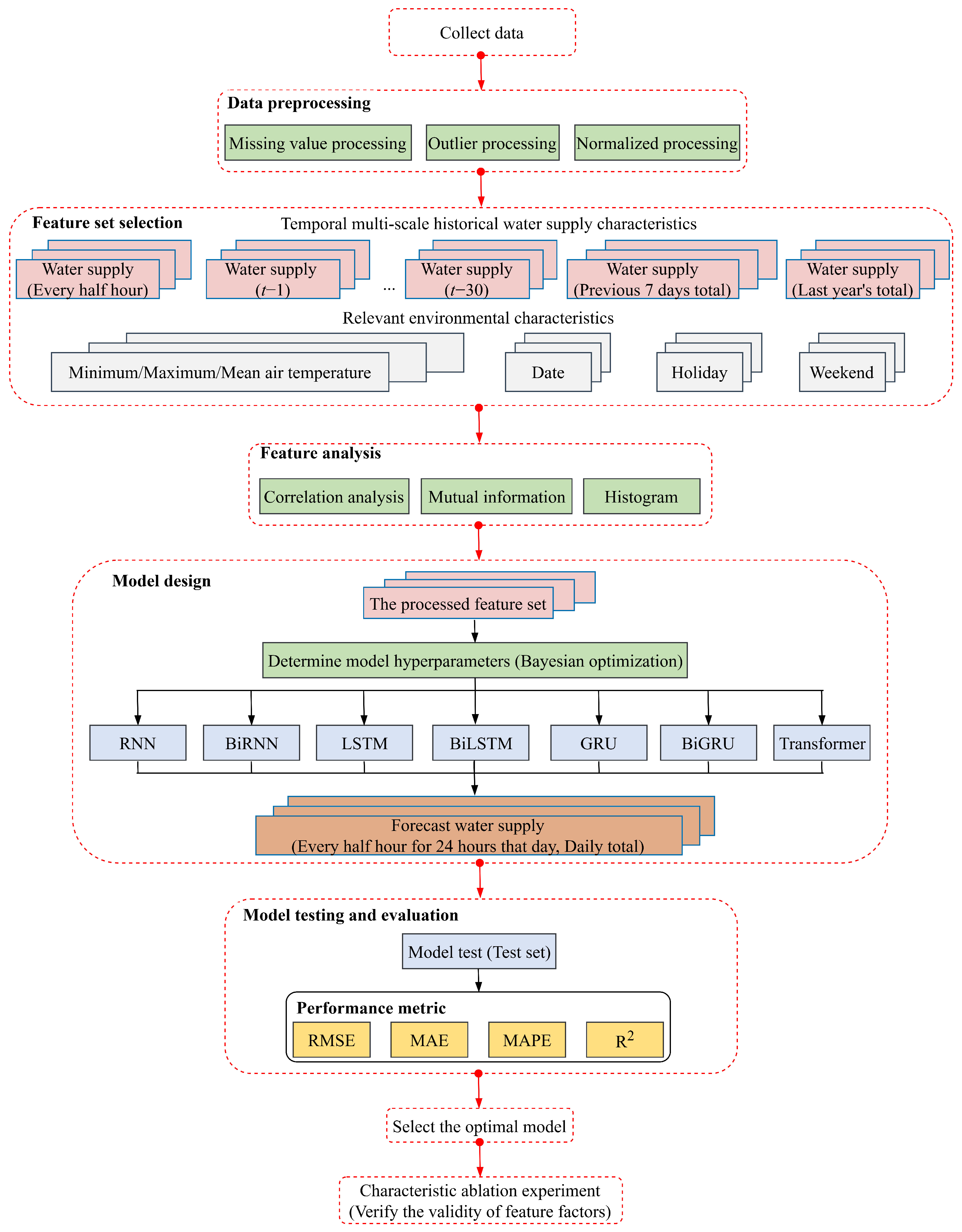Figure 1 globally presents the flowchart of this study, which includes data preprocessing, feature extraction and correlation analysis, hyperparameter tuning, model training, and model evaluation.

The main contributions of this study are as follows:

• In view of the existing problem of insufficient research on historical water supply data in the current field of water supply prediction, this study considers the selection of historical water supply characteristic factors from the perspective of multi-time scales, and extracts a series of characteristic factors (TMFs) with different time spans to form a characteristic set, and experimentally proves the effectiveness of this characteristic set.
• In order to deal with the problem of changes in the time cycle factors of water supply prediction brought about by social development, this study proposes to conduct ultra-short-term water demand forecasting (UWDF) of water supply, which can better match the actual dynamic changes, achieve more refined water supply control, and improve the reliability and stability of water supply.
• Feature selection and model selection are the most important aspects of the water supply prediction task. In this study, various methods in feature engineering are used to comprehensively analyze the selected feature set, verifying the correlation and potential relationship between the selected feature set and the water supply in this study, and comparing and analyzing the prediction performance of seven deep learning models such as RNN, providing guidance for subsequent domain research.

The rest of this study is organized as follows: Section 2 illustrates the selection methods for the feature sets and models used in water supply volume prediction. Section 3 describes the relevant experiments conducted in this research and their results. Section 4 presents the research conclusions.

2. Methodology

2.1. Data Preprocessing

This study was carried out based on a water plant in a county town in China. The water supply capacity of this plant is approximately 30,000 cubic meters per day, mainly serving the county town area, with a total supply population of about 195,000 people.

In this study, we collected half-hourly and total daily water supply data for a water treatment facility in Chongqing Municipality from January 2019 to April 2022. The dataset is refined by employing the traditional mean interpolation technique to address missing values and outliers. The mean interpolation method is a widely used approach for handling anomalous data, which estimates missing and outlier values based on the average of the feature values. The process includes the following steps:

• Identify the missing values and outliers in the dataset, which are usually represented by a specific symbol (NaN, None, etc.).
• Calculate the mean value of non-missing or non-outlier values for each feature, which will be used to replace the missing and outlier values in the corresponding feature.
• For each missing value and outlier, replace it with the mean value of that feature.

After addressing missing values and outliers, the data are normalized, a crucial step that reduces scale disparities among different features, allowing for direct comparison and improving the model’s convergence speed. Common normalization methods include min-max scaling, standardization, and custom scaling. In this study, we employ the min-max scaling technique to standardize the data. The preprocessed water supply data for the water plant are illustrated in Figure 2.

Through the preliminary analysis of these data, we generally understand the water supply rules and characteristics of this water plant. The water supply volume shows a trend of increasing year by year and has obvious seasonal variations. For example, by comparing the data of 2019 and 2022, the increase in the water supply volume can be clearly seen, which is closely related to urban construction, the improvement of the residents’ living standards, and the development of industrial production. From a seasonal perspective, water consumption is significantly affected by seasonal factors. In summer, due to the relatively high temperature, the residents’ water demand increases, mainly for daily life water use such as cooling and bathing, and the cooling water demand in some industrial production also rises, resulting in a corresponding increase in the water supply volume. In winter, the water consumption is relatively reduced, but in some special cases, such as the use of heating equipment, it may increase the water consumption to some extent.

2.2. Feature Set Selection

The water supply forecast model features two primary components: historical water supply data and pertinent environmental factors. These elements are chosen with a dual consideration of the immediate influences on water supply, as well as the long-term impacts stemming from economic, social, and urban development trends. For instance, as China is undergoing rapid urbanization, the annual water consumption is continuing to rise. Figure 1 illustrates that the projected water supply for 2022 is notably higher than that of 2019.

Scholars, including Kim et al. [10], have underscored the significance of incorporating both historical water usage data and environmental characterization factors when forecasting various types of water usage to enhance prediction accuracy. However, a deeper analysis suggests that many researchers in the field of water supply forecasting have predominantly focused on selecting environmental factors while overlooking the extraction and analysis of historical water supply data. For example, Xenochristou et al. [13] used a number of environmental characterization factors, such as seasons, in order to predict the water demand in different time scales but only considered historical water use data in the selection of the water use data for the previous 7 days. The methodology proposed by Rasifaghihi et al. [15] focused only on the effect of climatic variables on water use. Ghannam et al. [16] employed multiple environmental factors, including temperature, to forecast urban water supply for multiple days ahead, yet they did not delve into the study of historical water supply data. In light of these findings, this study revisits the significance of both historical water supply data and related environmental factors, reassessing their importance in the selection and analysis process for a more comprehensive and robust water supply forecast model.

2.2.1. Time Multi-Scale Historical Water Supply Characterization

In this study, the selection of factors characterizing historical water supply is considered from a time multi-scale perspective. In time series analysis and prediction, considering the change patterns of multiple time scales [17] is also one of the keys that affect the prediction results because it can capture the changing laws of data under different time scales. It covers different time dimensions, including long-term trends, medium-term fluctuations, short-term dynamic changes, etc. In the context of water supply volume prediction, such multi-scale considerations can acutely capture the unique changing laws contained in the data under different time spans. By incorporating features of multiple time scales, the model can gain an in-depth understanding of the complex internal logic of changes in water supply volume, and then significantly improve the accuracy and robustness of its prediction. Meanwhile, Niknam et al. [12] have pointed out that the paradigm of water supply forecasting time cycle factors has changed with the development of society, as the cycle is now shorter than hourly demand forecasting, and this change is crucial to understanding the new challenges of water demand forecasting methods.

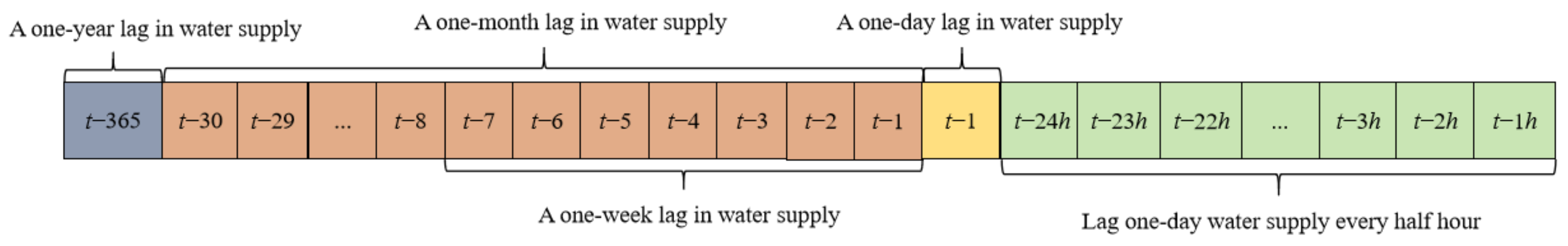
Therefore, starting from the perspective of multiple time scales and taking a comprehensive consideration of the existing literature on water supply volume prediction, this study extracts a series of feature factors with different time spans from the preprocessed historical water supply data, namely, the water supply volume lagged by one year, the water supply volume lagged by one month, the water supply volume lagged by one week, the water supply volume lagged by one day, and the water supply volume lagged by half an hour per day.

2.2.2. Externally Relevant Environmental Characteristics

Regarding the selection of relevant environmental characteristic factors, this study thoroughly examines the literature on water supply prediction. It identifies external environmental factors that significantly influence water supply forecasting, such as the date, holidays, daily minimum temperature, daily maximum temperature, and daily average temperature. These factors are chosen as the characteristic indicators for this study.

These characteristic factors serve as model inputs to predict water supply over the ultra-short term. This approach addresses the issue of timeliness that is often lacking in hourly based water demand forecasts, a challenge exacerbated by the rapid pace of social and economic development. Furthermore, by leveraging historical water supply data, the model aims to offer more precise, effective, and real-time water resource planning for water supply facilities. This ensures that water management can be proactively adjusted to meet immediate and future demands.

2.3. Feature Correlation Analysis

In order to verify the correlation and potential relationship between the selected feature set and water supply in this study, the feature engineering methods commonly used in the water supply literature, i.e., correlation analysis (CA) [18,19], mutual information (MI) [20], and histograms, are chosen to perform a comprehensive analysis of the selected feature set. Feature correlation analysis can help to understand the relationship between the features in the dataset and better reveal the intrinsic structure and patterns of the dataset.

For the sake of clarity and ease of representation, each feature factor within the feature set is relabeled, as detailed in

Table 1. Renaming feature variables.

Characteristic Category	Variable Name	Rename
Time multi-scale characteristics	Water supply with 1 year lag	YLWS
	Water supply with 1 month lag	MLWS
	Water supply with 1 week lag	WLWS
	Water supply with 1 day lag	DLWS
	Water supply per half hour on 1 day lag	HHLWS
Relevant environmental characteristics	Daily Minimum Temperature	Min_T
	Daily Maximum Temperature	Max_T
	Average Daily Temperature	Ave_T
	Holiday	H
Target variable	Water supply	WS

. This relabeling facilitates a more straightforward analysis and interpretation of the data.

Figure 3 presents a visual representation of the historical water supply feature factors across different time scales. This visual depiction aids in recognizing the temporal dynamics of the water supply patterns and provides a clear overview of how the selected features are distributed and interact with each other over time.

2.3.1. Correlation Coefficient Analysis

The correlation between features and water supply is pivotal for the accurate prediction of water supply levels. By examining the correlation coefficients between the feature factors and water supply, as discussed by [21,22], one can swiftly gauge the linear or nonlinear relationships at play. This assessment is invaluable for uncovering potential patterns and structures within the dataset. Identifying features with a high correlation to water supply is essential for constructing a more precise and dependable water supply forecasting model. It allows for the selection of the most influential factors, which in turn enhances the model’s predictive power and reliability. This approach ensures that the model is grounded in a solid understanding of the data’s inherent relationships, leading to more informed and accurate water supply predictions.

In this study, we utilize several statistical measures to analyze the correlation between the characteristic factors and water supply quantity. The four correlation coefficients employed and their interpretations are as follows:

• Pearson correlation coefficient: This measures the degree of linear correlation between two continuous variables. It assumes that the relationship between the variables is linear and requires that the variables should be normally or approximately normally distributed.
• Spearman’s correlation coefficient: This measures the monotonic relationship between two variables and does not require that the variables be continuous or conform to a specific distribution. It measures the relationship between variables by converting the raw data to rank order.
• Kendall’s correlation coefficient: This is also a measure of the monotonic relationship between two variables and is similar to Spearman’s correlation coefficient. The difference is that the Kendall correlation coefficient takes into account the rank relationship between the variables rather than specific values.
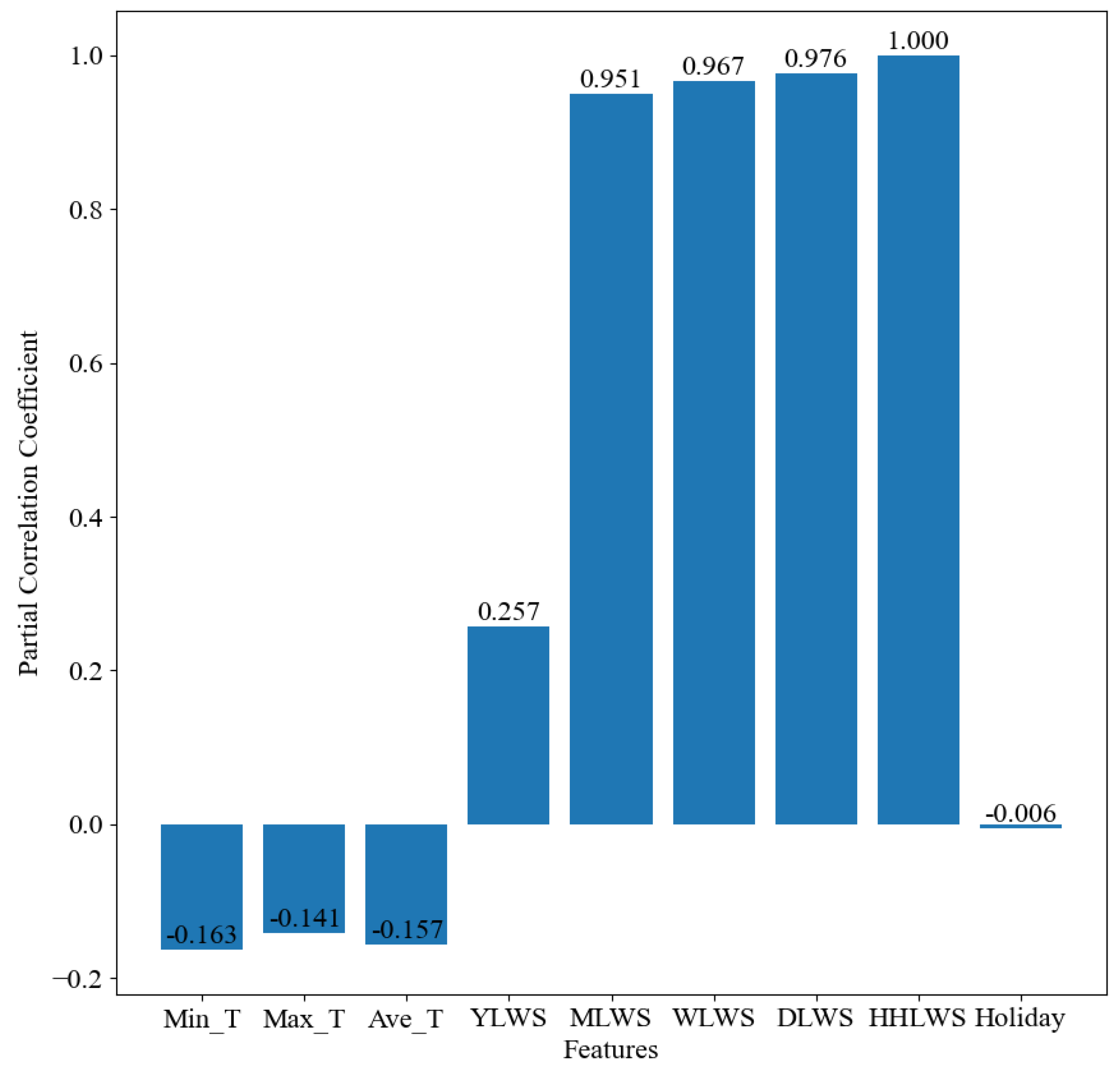
• Partial correlation coefficient: This measures the correlation between two variables controlling for the influence of other variables. In multivariate statistical analysis, the partial correlation coefficient is used to eliminate the effects of other variables to more accurately assess the relationship between two variables.

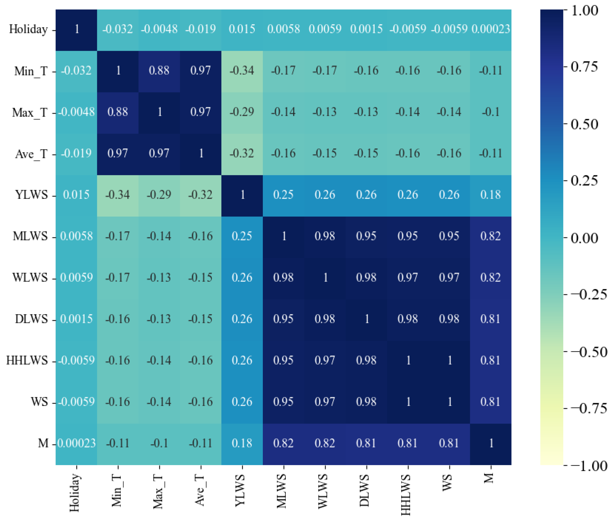
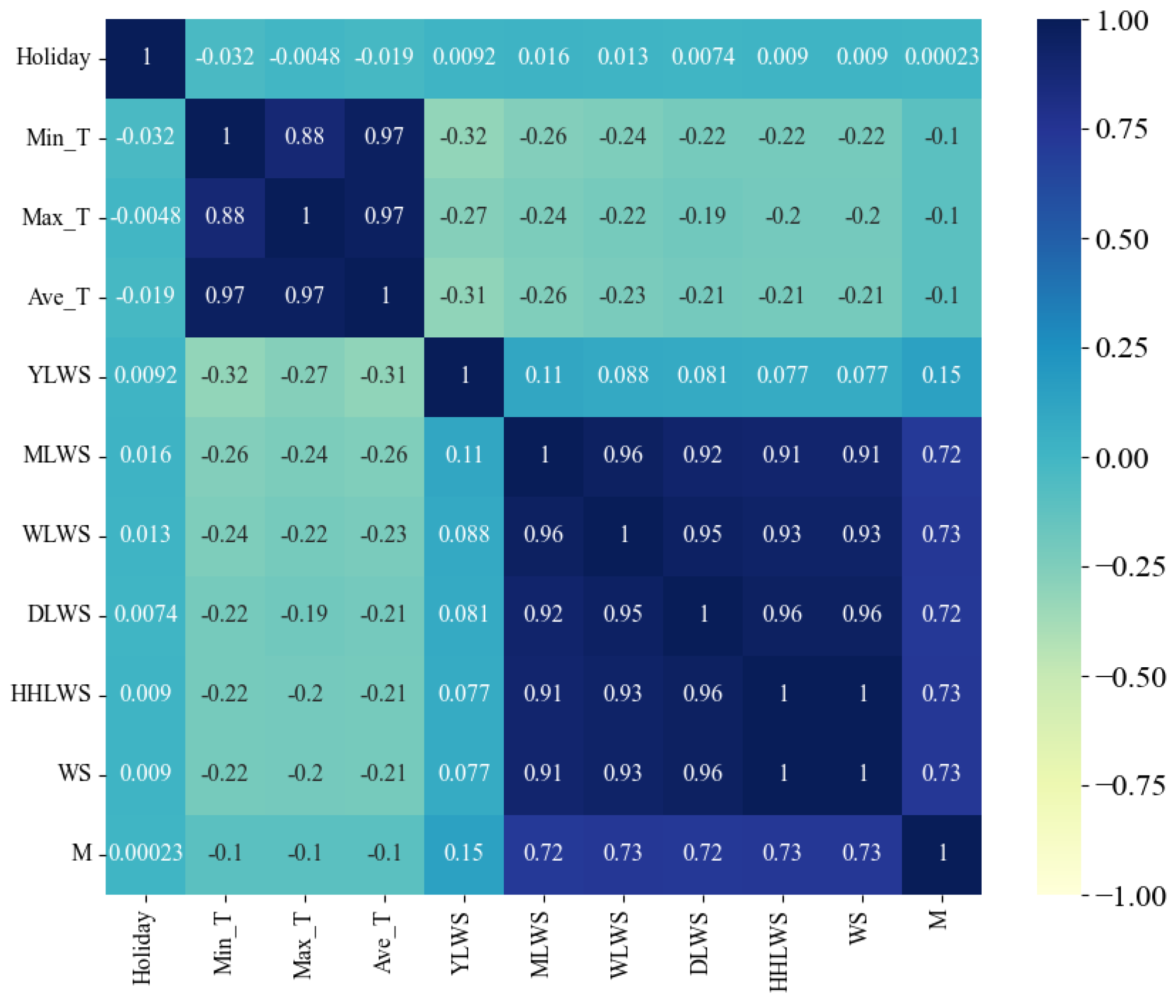
Figure 4, Figure 5, Figure 6 and Figure 7 present heat maps illustrating the Pearson correlation coefficient, Spearman correlation coefficient, Kendall rank correlation coefficient, and partial correlation coefficient, respectively. These visual representations provide a clear and concise overview of the strength and direction of the relationships between the variables, facilitating a better understanding of the underlying data dynamics.

Upon examining the figures, it is evident that the feature variables proposed in this study, which pertain to historical water supply data, exhibit a correlation with the water supply quantity. Notably, the feature factors representing the water supply quantities from the previous month, the previous week, the previous day, and the previous half hour of the previous day demonstrate a strong positive correlation (correlation coefficients > 0.75). This finding substantiates the effectiveness of the multi-scale temporal feature factors selected. The correlation coefficients for the environmental factors are found to be lower than those for the historical water supply data, suggesting that water supply predictions are more heavily reliant on historical water supply data rather than external environmental factors.

In addition, we also discover two interesting phenomena. Firstly, the correlation coefficients of the three feature factors, namely, the minimum temperature (Min_T), the maximum temperature (Max_T), and the average temperature (Ave_T), show a low negative correlation in all four correlation analysis methods. However, in the correlation analyses of other water supply volume prediction literature [12,16], these feature factors all show a positive correlation. It is speculated that the reason for this problem may be that, due to the differences in research objects, the impacts of feature factors also vary accordingly. Compared with other studies, although the research goal of this study is also water supply volume prediction, the research objects of other studies are cities, regions, or households, while the research object of this study is the water supply volume prediction for water plants. It is also possible that this is caused by regional differences. Because the average annual temperature in the research area of this study is relatively low, it has led to the analysis result that the water supply volume is less affected by environmental factors such as temperature.

Secondly, the low correlation shown between the holiday feature factor and the water supply volume is worthy of in-depth discussion. The reason may be that the water supply of this water plant is mainly divided into three main parts: municipal, industrial, and residential water use. During holidays, the situation of residential water use changes. Some residents spend more time at home, resulting in an increase in the frequency of daily water use activities such as laundry and cooking, and the water demand increases to some extent. However, in terms of industrial water use, as many units are on holiday and suspend work, the industrial water consumption usually decreases significantly. Municipal water use is also adjusted due to changes in the rhythm of urban operation during holidays. Although residential water use increases during holidays, the significant reductions in industrial and municipal water consumption are even greater such that the overall change in water consumption is not significant, finally leading to the low correlation between holidays and the total water supply volume.

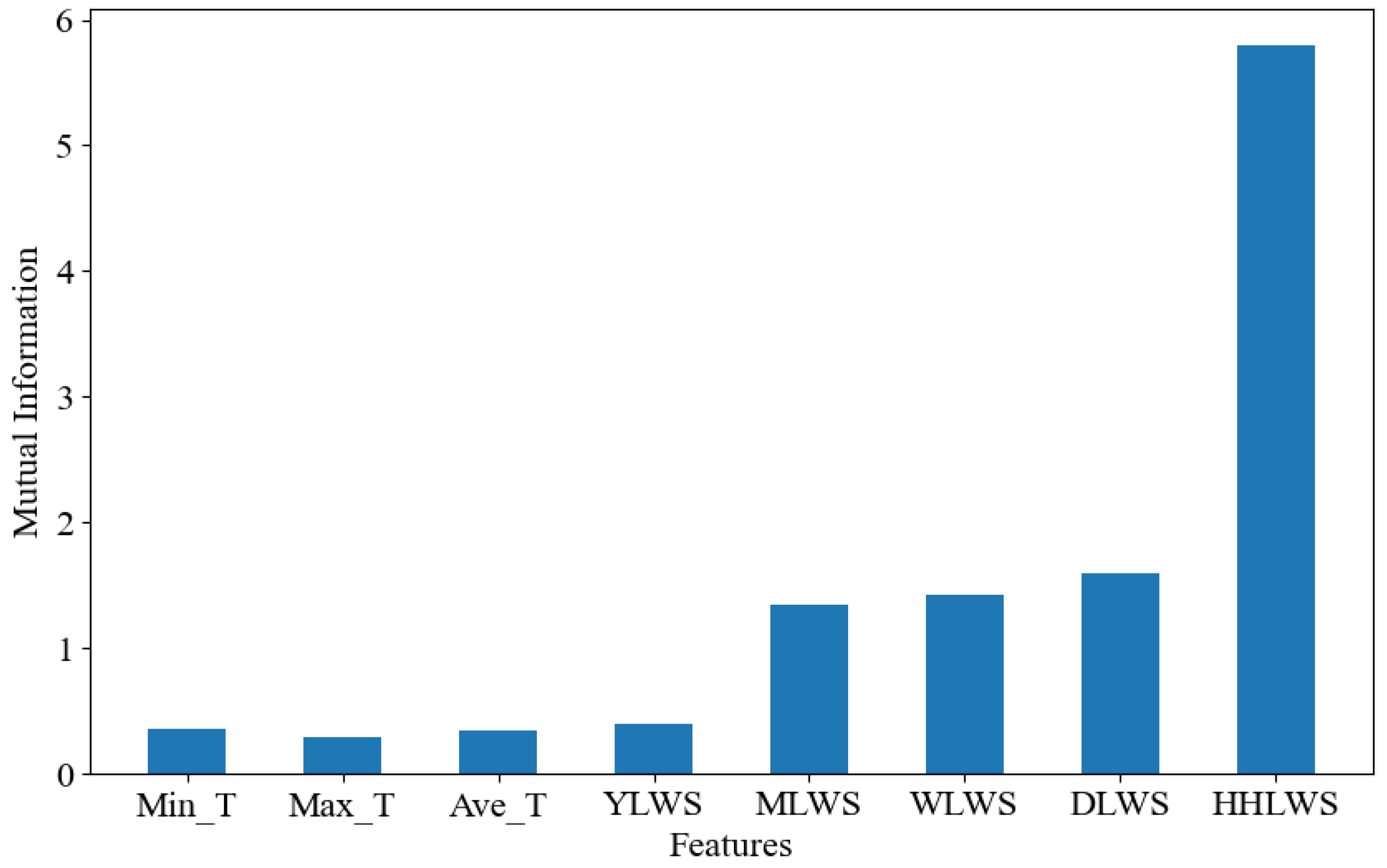
2.3.2. Mutual Information Analysis

Mutual information is a measure of the degree of association between two random variables; it measures the degree to which the amount of information in one random variable affects the other random variable, and by calculating the value of mutual information, it can help to understand the degree of correlation between features. Mutual information is defined as follows.

Suppose there are two continuous random variables X and Y with joint probability distribution $P(x,y)$ and marginal probability distribution $P\left(x\right)$ and $P\left(y\right)$, respectively. Then, the mutual information $I(X;Y)$ is

$$I(X;Y)=\sum _{y\in Y}\sum _{x\in X}p(x,y)log\left({\displaystyle \frac{p(x,y)}{p\left(x\right)p\left(y\right)}}\right)$$

(1)

The mutual information values of each characterization factor for the target variable (water supply quantity) are calculated using the mutual information method, and the results are shown in Figure 8. Similar to the conclusions drawn from the correlation analysis, the eigenfactors of the water supply with a lag of 1 week, water supply with a lag of 1 month, water supply with a lag of 1 day, and water supply with a lag of 1 day for every half hour show high mutual information values, with the mutual information value of water supply with a lag of 1 day for every half hour being particularly prominent, indicating that the prediction of the target variable (water supply) is strongly influenced by this eigenfactor, while the other eigenfactors factors all have mutual information values ≥ 0, which are dependent on the target variable and are included in the input feature set of the model to improve prediction accuracy.

2.3.3. Histogram of Features

Histograms provide a clear picture of the distribution of the data and an understanding of the central tendency, degree of dispersion, and shape of the data. Figure 9 illustrates the histogram of each feature factor in the feature set. The histogram clearly and intuitively reveals that the distribution of all remaining feature factors, with the exception of air temperature, approximates a Gaussian distribution. This characteristic is beneficial, as it simplifies the modeling process and facilitates a more precise model fit.

2.4. Model Selection

In the process of model selection, the studies conducted by Kavya et al. [11], Koo et al. [14], and Kim et al. [10] demonstrated that deep learning models surpass traditional statistical and machine learning models in terms of efficiency and accuracy when dealing with time series data in water demand forecasting. Deep learning models excel at extracting complex features from raw data, which enables them to capture intricate patterns and underlying rules within the data. These models are also known for their flexibility and adaptability to various types and lengths of sequence data. Given these advantages, this study opts for deep learning models for the water supply prediction study and compares their performance. The models select include the Recurrent Neural Network (RNN), Bidirectional Recurrent Neural Network (BiRNN), Long Short-Term Memory Network (LSTM), Bidirectional Long Short-Term Memory Network (BiLSTM), Gated Recurrent Units (GRUs), Bidirectional Gated Recurrent Units (BiGRUs), and Transformer models. These models are particularly adept at handling sequence data due to their enhanced processing capabilities. They are also proficient in managing long-term dependencies within sequence data. These models maintain a memory of past information and apply it to the current prediction task, which allows them to better capture temporal dependencies in the data. By leveraging these deep learning models, the study aims to develop a robust water supply prediction framework that can effectively model complex temporal dynamics and improve the accuracy of forecasting efforts.

2.4.1. Recurrent Neural Network

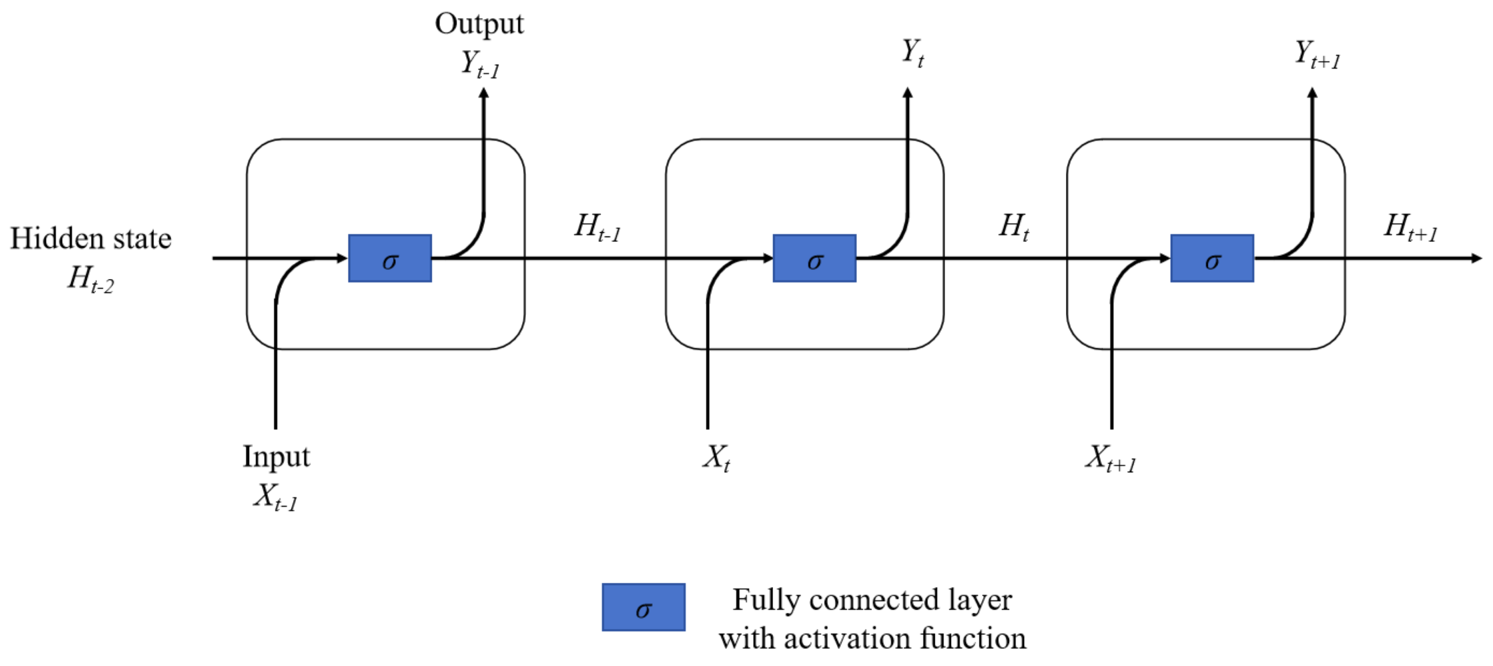
Recurrent Neural Networks have strong model-fitting abilities for serialized data. The presence of recurrent connections between neurons in the hidden layer of the RNN [23] allows the network to store past information in the hidden state and apply it to the current inputs and outputs. Specifically, a Recurrent Neural Network (RNN) takes the current input and the hidden state from the previous time step as inputs at each time step, subsequently generating the output for the current time step and a new hidden state. This recurrent architecture enables the RNN to process sequences of an arbitrary length and to capture long-term dependencies within those sequences. The structure of the basic unit of the RNN is illustrated in Figure 10.

Where $x_t$ represents the sample input (N-dimensional features) at the current moment t, $y_t$ represents the output at the current moment, and $H_t$ represents the hidden state at the current moment t. The computation is performed based on the output of the current input layer and the state of the hidden layer in the previous step:

$$H_t=f(U\ast x_t+W\ast H_{t-1})$$

(2)

where f is typically a nonlinear activation function such as tanh or ReLU.

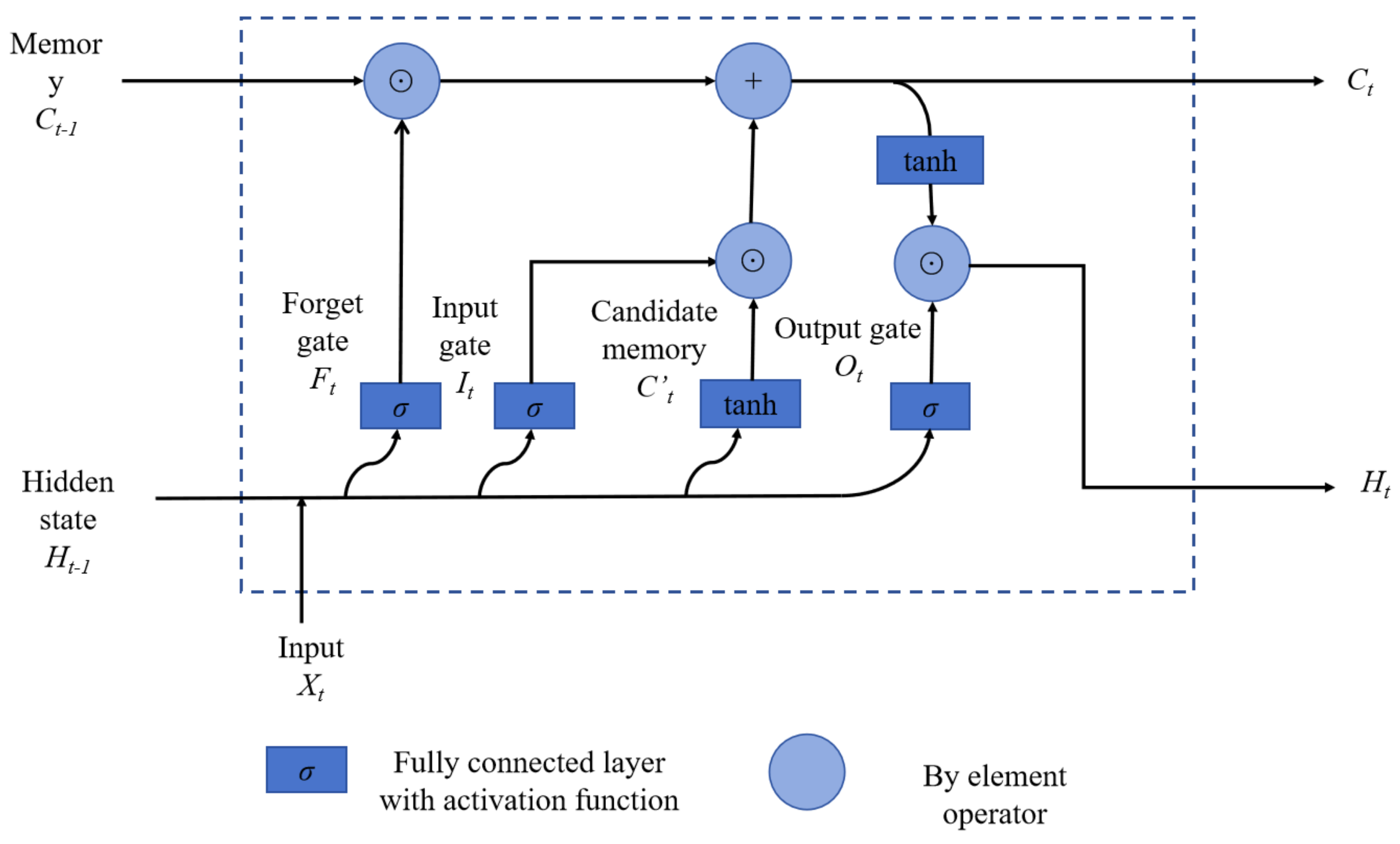
2.4.2. Long Short-Term Memory

LSTM [23,24] is a classical Recurrent Neural Network structure proposed for the long- and short-term dependencies of data, and its basic units can add and forget previous input information through the internal gate structure, including forgetting gates, input gates, and output gates. The basic unit structure of LSTM is shown in Figure 11.

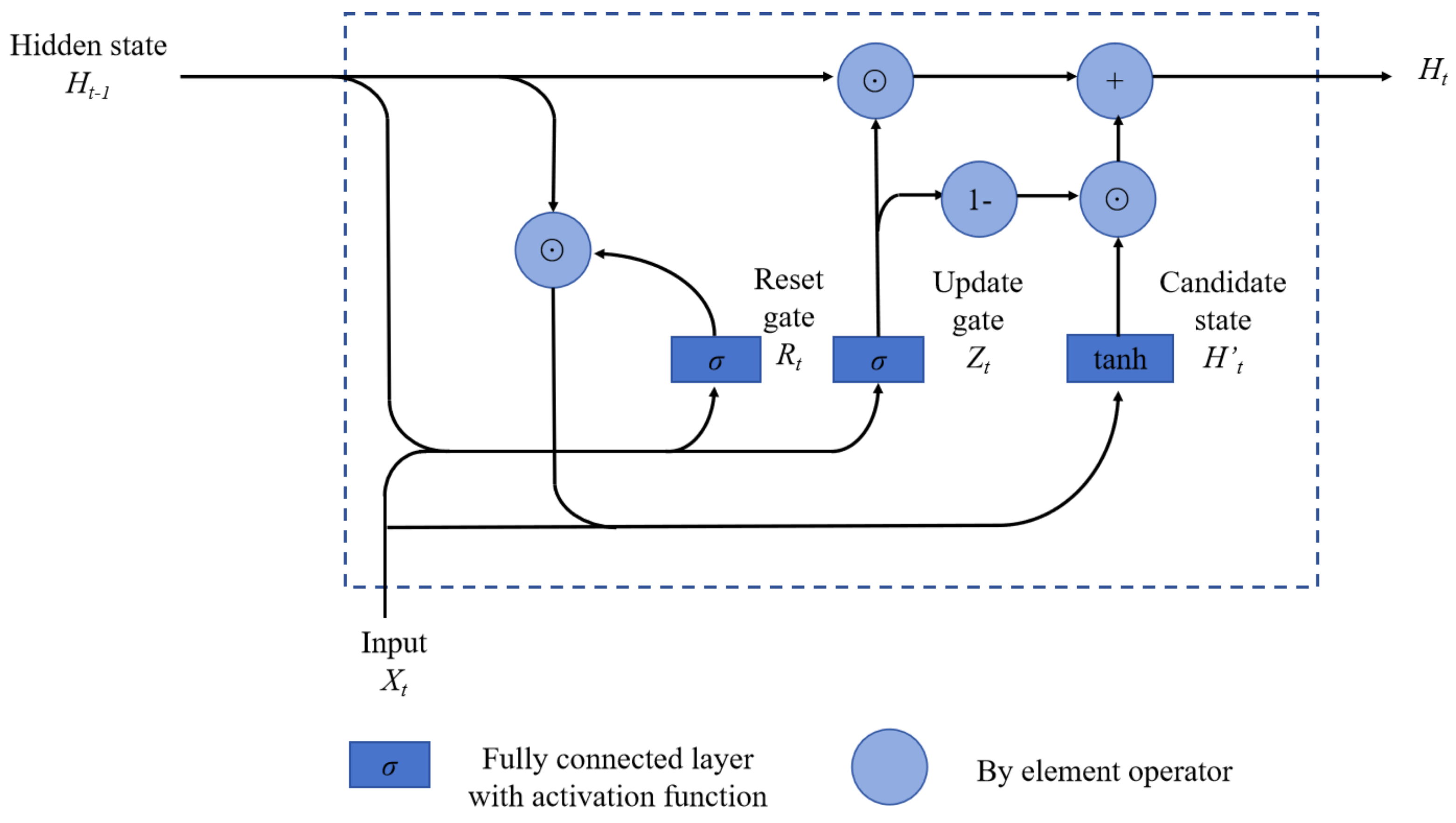
2.4.3. Gated Recurrent Unit

GRU [25] is a special type of Recurrent Neural Network that utilizes a gating mechanism to control the flow of information in a sequence. Compared to LSTM, GRU removes the structure of the state and instead introduces reset and update gates. The reset gate determines how much previous information is retained in the current time step, and the update gate controls whether to update the state of the current time step. The unit structure is shown in Figure 12 below.

2.4.4. Transformer

Transformer is a deep learning model for processing sequence data, proposed by Vaswani et al. [26] The core idea is to model sequences by capturing the dependencies between positions in the sequence through a self-attention mechanism.

The self-attention mechanism enables the model to consider information from other positions in the sequence when processing each position’s input, facilitating global information exchange. It achieves a comprehensive sequence representation by calculating the correlation between each position and others, applying weights, and summing the information from various positions to form a representation for that specific position. This mechanism allows the model to more effectively capture long-distance dependencies within the sequence, enhancing its modeling capabilities.

2.5. Model Hyperparameter Selection

In machine learning, a model’s performance and generalization are often influenced by the selection of hyperparameters. These are parameters set before training the model that dictate its architecture and the rules for parameter updates during training, such as the learning rate and the number of neurons in the hidden layers. Traditionally, hyperparameter selection relies on a researcher’s domain knowledge or experience, which can be labor intensive and does not guarantee the optimal choice for the model. For instance, a learning rate that is too high might prevent the model from converging, while a rate that is too low can lead to slow training progress.

With the development of technology, the application of hyperparameter tuning techniques solves the above problems. The hyperparameter tuning technique is the process of improving the performance and generalization ability of a model by systematically searching for and selecting the optimal combination of hyperparameters. Different combinations of hyperparameters may lead to significant changes in model performance, and better performance and generalization can be achieved by constantly adjusting the hyperparameters to find the most suitable combination of parameters for the model. Commonly used hyperparameter tuning techniques include grid search (GS), random search (RS), Bayesian optimization (BO), genetic algorithm (GA), and heuristic search (HS).

In this study, the Bayesian optimization technique [27] is chosen for hyperparameter tuning. In hydraulic systems, parameters such as water flow velocity and pressure exhibit certain uncertainties. Additionally, parameters like hydraulic conductivity and pipe roughness play a vital role in influencing the water supply volume in hydraulic calculations. The Bayesian approximation method is capable of quantifying these uncertainties by establishing a probability model and fully taking their impacts into account during the hyperparameter optimization process. Compared with traditional grid search and random search, Bayesian optimization not only estimates the probability distribution of the target function by setting up a probability model but also considers the uncertainty of the target function at the same time. It meticulously selects the next hyperparameter combination to be evaluated based on the current estimated distribution. This enables it to efficiently identify a relatively superior hyperparameter combination within a relatively small number of iterations, effectively saving time and reducing costs. Moreover, the adaptability of Bayesian optimization empowers it to flexibly adjust the next selected hyperparameter combination according to previous observation results, thereby searching for the optimal solution in a more intelligent way. In the context of hydraulic systems, this adaptability implies that it can dynamically adjust the search strategy in line with the uncertainty characteristics of hydraulic-related parameters. This allows the model to better adapt to the complexity of the hydraulic system when choosing hyperparameter combinations, and consequently, enhance the accuracy and reliability of the water supply volume prediction model.

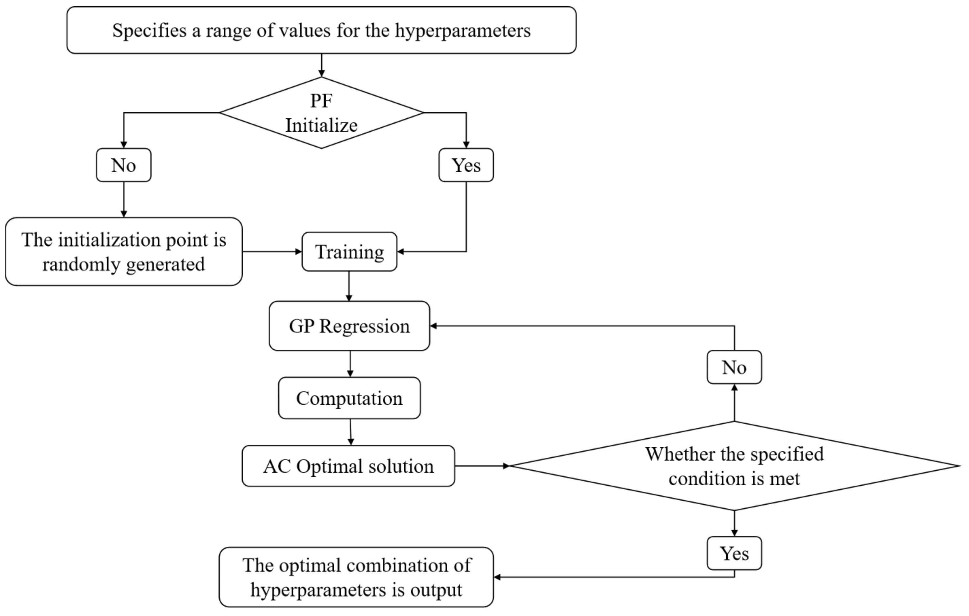
Figure 13 depicts the general process of Bayesian optimization for hyperparameters, in which the two most important components are PF (prior function) and AC (acquisition function):

• PF: If the function distribution is known, the optimal model is selected empirically. If unknown, a kernel function based on Gaussian process is used as a black-box function for self-learning.
• AC: It is used to search for the extreme value point of the objective function, and then this extreme value point is used as input for a machine learning or deep learning model to predict a result. This result is updated to the Gaussian distribution model in the previous step.

The model hyperparameters in this study consist of four main ones, which are the learning rate, the number of hidden layer layers, the number of neurons in the hidden layer, and the number of training rounds. They are renamed separately for ease of representation as shown in

Table 2. Hyperparameter renaming.

Hyperparameters	Rename
Learning rate	learning_rate
Number of hidden layers	num_layers
Number of neurons in hidden layer	hidden_size
Iteration rounds	num_epochs

.

2.6. Model Training

This subsection focuses on the details related to the model training phase. In this study, the dataset is divided into a training set, a validation set, and a test set. In total, 90% of the data from the dataset is divided as a training set for training the model, 10% of the data from the training set is taken as a validation set for model hyperparameter tuning, and the remaining 10% is taken as a test set for evaluating the model performance. The reason for such a division is that although the collected data span several years in terms of time, they are still relatively limited compared to some large-scale datasets. Under such circumstances, in order for the model to fully learn the feature representations in the water supply volume data, as many samples as possible are needed for training. Allocating 90% of the data to the training set can make the best use of the existing data, enabling the model to be exposed to more diverse patterns of water supply volume changes, historical water supply characteristics, and information related to external environmental factors. With a limited amount of data, the division of 10% for the test set can not only conduct a relatively reasonable assessment of the model’s performance but also avoid sacrificing the amount of data in the training set excessively.

In the model training phase, the Bayesian optimization technique is used to determine the optimal model hyperparameters for each of the seven models. The processed feature factors plus dates are then used as inputs to the seven deep learning models to make ultra-short-term water supply demand predictions, i.e., predicting the amount of water to be supplied by the water plant for each half hour of the 24 h period on the same day and the total amount of water to be supplied on the same day (49 dimensions in total).

In addition, all seven models are trained using mean square error (MSE) as the loss function and Adam as the optimization algorithm. RNN, LSTM, and GRU use tanh as the activation function for the hidden layer, and Transformer uses ReLU as the activation function for the hidden layer, whose number of attention heads is set to 11. The MSE is calculated as follows:

$$Los{s}_{MSE}={\displaystyle \frac{1}{n}}\sum _{i=1}^n{(y_i-{\widehat{y}}_i)}^2$$

(3)

where n is the number of samples, $y_i$ is the true value of the ith sample, and ${\widehat{y}}_i$ is the predicted value of the model for the ith sample.

2.7. Performance Metrics

Performance metrics are essential for evaluating a model’s effectiveness in prediction or classification tasks. They offer a numerical measure of the model’s predictive outcomes, aiding in the comprehension, comparison, and contrast of various models’ accuracy, stability, and generalization capabilities. Various performance metrics can highlight different facets of a model’s performance.

In the model evaluation stage, this study selects four performance metrics that are commonly used in the field of short-term water supply forecasting [28], i.e., root mean square error (RMSE), mean absolute error (MAE), mean absolute percentage error (MAPE), and goodness-of-fit (R²), to evaluate the prediction performance of the seven deep learning models on the test set and to select the optimal model. The formulas for the above performance metrics are given below:

$$\mathrm{RMSE}=\sqrt{{\displaystyle \frac{1}{n}}\sum _{i=1}^n{\left(y_i-{\widehat{y}}_i\right)}^2}$$

(4)

$$\mathrm{MAE}={\displaystyle \frac{1}{n}}\sum _{i=1}^n|y_i-{\widehat{y}}_i|$$

(5)

$$\mathrm{MAPE}={\displaystyle \frac{1}{n}}\sum _{i=1}^n\left|{\displaystyle \frac{y_i-{\widehat{y}}_i}{y_i}}\right|\times 100\%$$

(6)

$${\mathrm{R}}^2=1-{\displaystyle \frac{{\sum }_{i=1}^n{\left(y_i-{\widehat{y}}_i\right)}^2}{{\sum }_{i=1}^n{\left(y_i-\widehat{y}\right)}^2}}$$

(7)

where n is the number of samples, $y_i$ is the true value, ${\widehat{y}}_i$ is the model predicted value, and $\overline{y}$ is the mean of the true value.

3. Experiments

3.1. Model Hyperparameter Tuning

In order to optimize the prediction performance of the model, hyperparameter tuning is needed to find the most suitable hyperparameters for the model before the model is trained. The Bayesian optimization technique is used to tune the hyperparameters of the RNN, LSTM, GRU, and Transformer models, respectively. The number of Bayesian optimization iterations is preset to 50, and the results are shown in

Table 3. Bayesian optimization results for hyperparameters.

Model	Learning_Rate	Num_Layers	Hidden_Size	Num_Epochs
RNN	1.135387 × ${10}^{-6}$	3	982	172
LSTM	1.073266 × ${10}^{-6}$	3	662	76
GRU	1.176652 × ${10}^{-6}$	3	610	74
Transformer	2.370798 × ${10}^{-6}$	4	719	99

.

At the same time, in order to verify the effectiveness of Bayesian optimization in selecting hyperparameters, we artificially set seven groups of hyperparameter values as a comparison based on relevant experience and domain knowledge. In order to facilitate the comparison, this study takes the LSTM model as an example, unifies the number of iteration rounds as 200 rounds, modifies the model hyperparameters to the following 8 groups of hyperparameters under the same training set (as shown in

Table 4. Hyperparameters of the LSTM model.

Model	Learning_Rate	Num_Layers	Hidden_Size	Num_Epochs
Artificially selected	1.000000 × ${10}^{-6}$	3	512	200
	1.000000 × ${10}^{-6}$	3	1024	200
	1.000000 × ${10}^{-6}$	4	512	200
	1.000000 × ${10}^{-6}$	4	1024	200
	1.000000 × ${10}^{-6}$	5	512	200
	1.000000 × ${10}^{-6}$	5	1024	200
	1.000000 × ${10}^{-6}$	6	512	200
Bayesian optimization	1.073266 × ${10}^{-6}$	3	662	200

), and records the average loss of the test set as the evaluation index. The results are shown in Figure 14.

The results show that the model hyperparameters selected by the LSTM model using Bayesian optimization (red curves) are better than those selected by human experience and reach the lowest average loss in the 62nd iteration round, with a value of 0.011908. It is observed that when a model has more than 3 network layers and the iterative training is just commencing, it exhibits a lower average loss. However, as the number of iterative training rounds increases, the model with more than 3 network layers begins to underperform compared to the model with exactly 3 network layers, and the overfitting phenomenon occurs sooner. This suggests that although deeper networks have more parameters and a greater capacity for feature representation, they can fit the training data more effectively in the early stages of training, hence showing a lower average loss. Yet, as training progresses, the complexity of deeper networks leads to earlier overfitting and the gradient updates during training can become either too small or too large. This hinders efficient parameter updates, adversely affecting the model’s performance and generalization capability. Consequently, in water supply prediction tasks, deeper networks do not necessarily result in superior performance but may instead heighten the risk of overfitting.

3.2. Model Evaluation

After determining the importance of model hyperparameter selection, this study uses seven deep learning-based neural network models, namely, Recurrent Neural Network (RNN), Bidirectional Recurrent Neural Network (BiRNN), Long Short-Term Memory Network (LSTM), Bidirectional Long Short-Term Memory Network (BiLSTM), Gated Recurrent Units (GRUs), Bidirectional Gated Recurrent Units (BiGRUs), and Transformer, with the same set of input features, to predict the 24-hourly half-hourly water supply of the day and the total water supply of the day for a water plant in Chongqing and to compare their model performance and generalization ability.

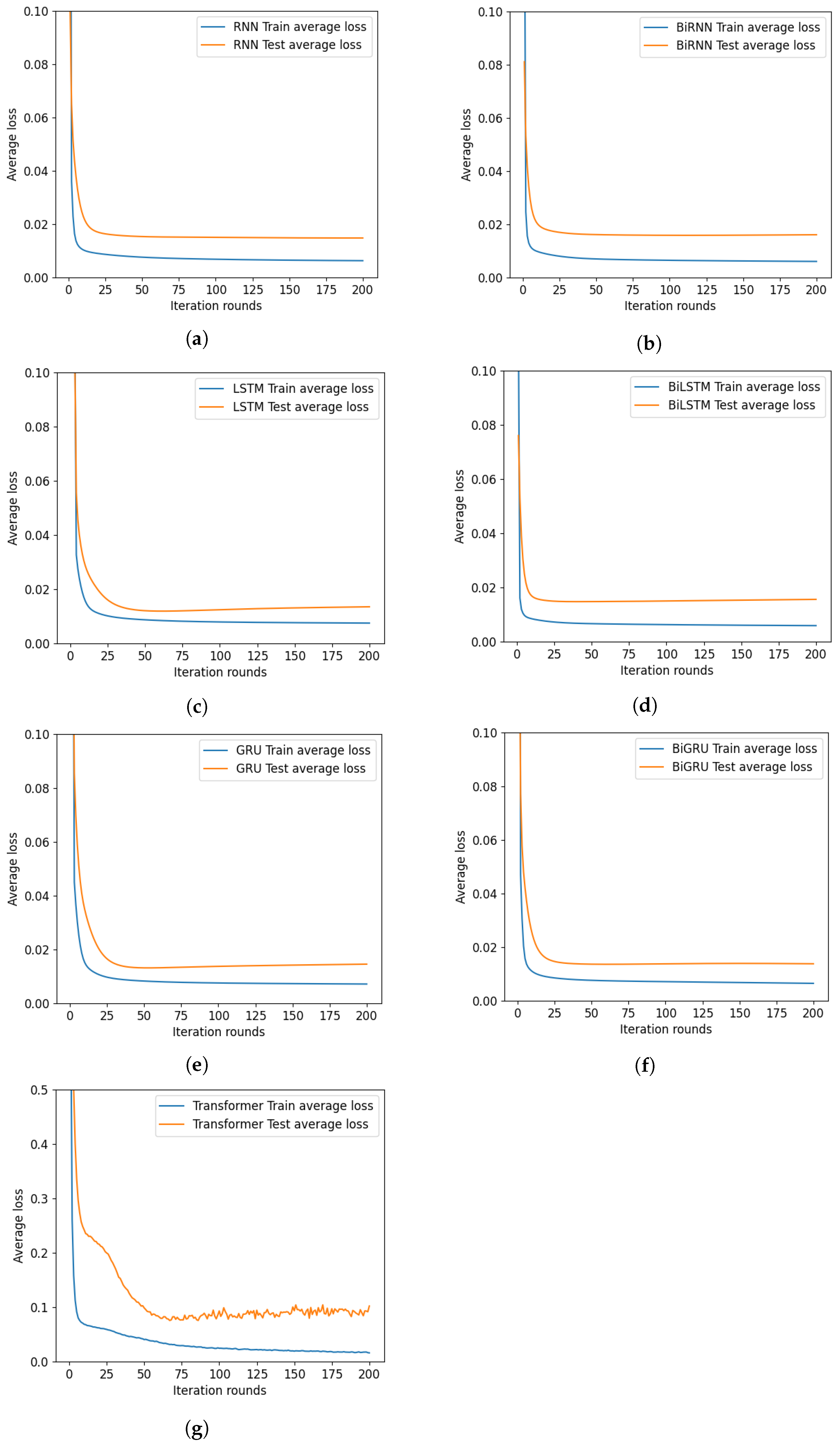
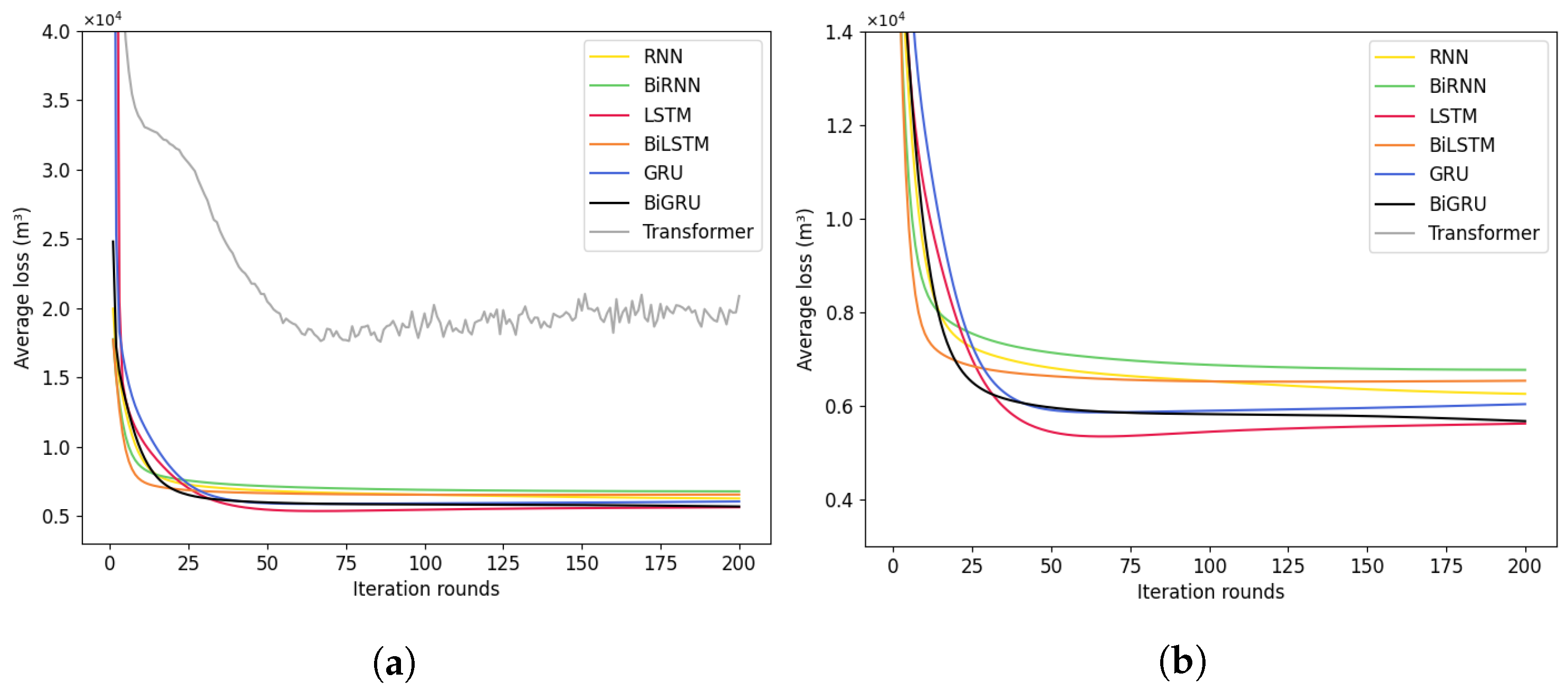
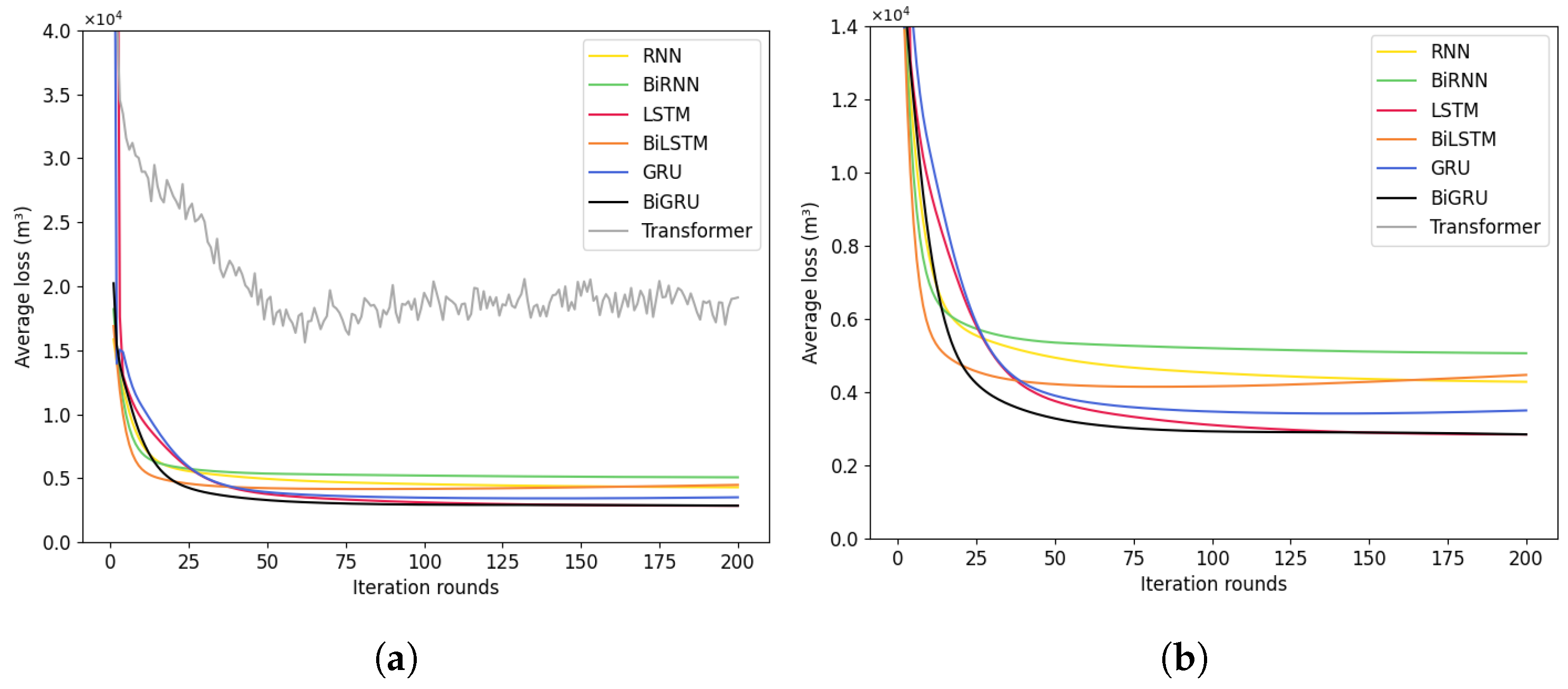
Again, the number of iterative training rounds is standardized to 200 for ease of observation, although the model may be overfitted due to too many iterations. Figure 15, Figure 16 and Figure 17 show the average loss curves of the training and test sets, the average loss curves of water supply per half hour, and the average loss curves of total water supply for the day for the seven deep learning models in each iteration round, respectively. The average loss curve of water supply per half hour and the average loss curve of total water supply on the same day are scaled on the y-axis to some extent for easy comparison. It is not difficult to observe from Figure 16b that as the number of iteration rounds increases, the average losses of the training sets of the seven deep learning models all decrease and converge. It is also found that except for the RNN model, the other models all have overfitting problems. However, these problems can be effectively resolved by controlling the number of iteration rounds or adding regularization techniques.

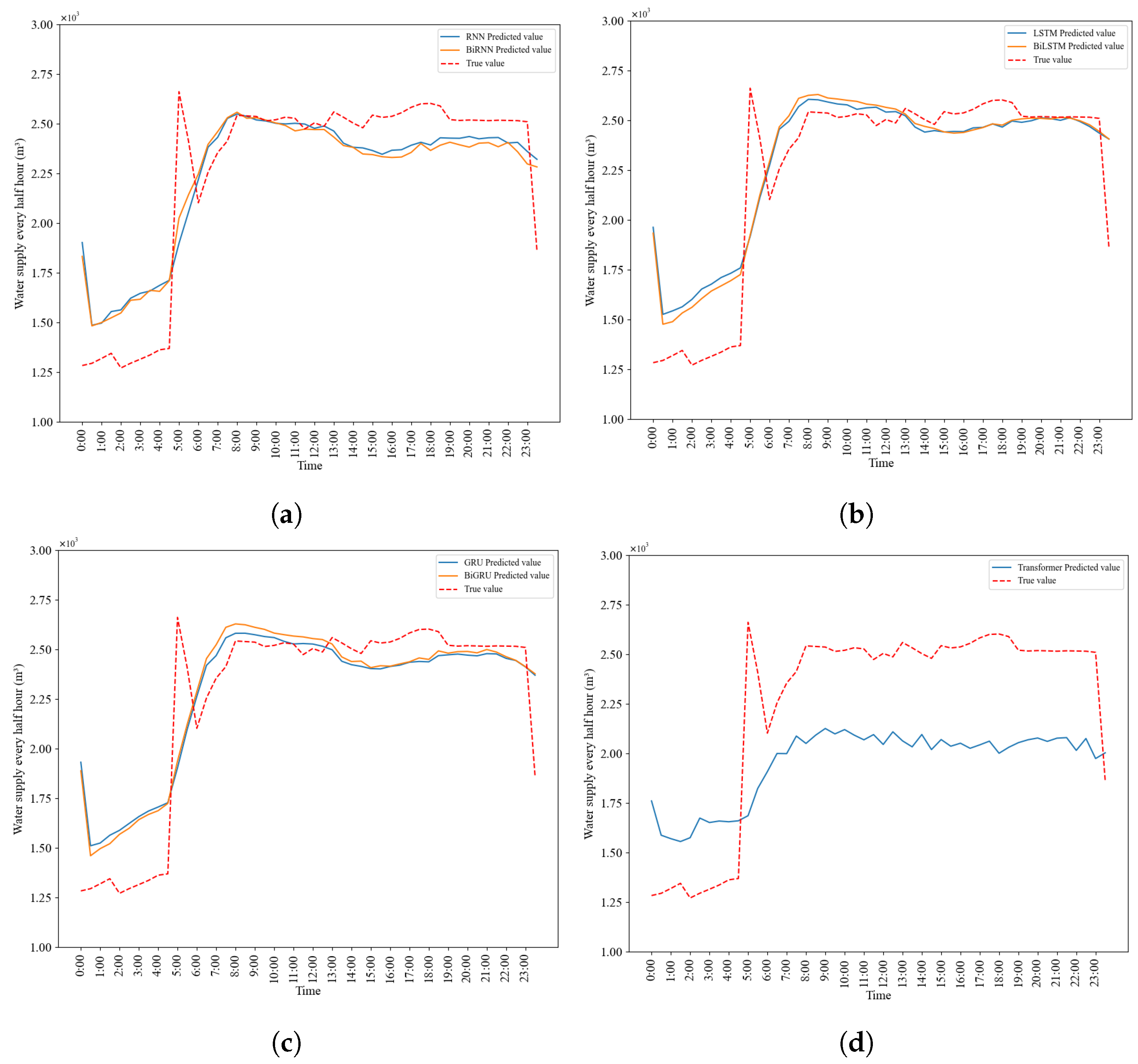
Figure 18 and Figure 19 intuitively demonstrate the consistency between the observed water supply volume per half an hour and per day in the next 100 days and the water supply volume per half an hour and per day predicted by the seven models. Among them, the LSTM and BiLSTM (Figure 18b and Figure 19b) models perform relatively well. The water supply volume per half an hour and the total daily water supply volume predicted by these models are closest to the actual values, and they also have good performance at the peak changes of the actual values.

In addition, it is observed in Figure 18 that the water supply curve predicted by the model during the period from 18:00 to 22:00 tends to be smooth, which seems unexpected but is reasonable according to the actual water supply data. The reason for this phenomenon may be that this period is usually the peak time for residential water use, and residents’ water use behaviors have a certain degree of regularity and stability. For example, during this period, residents mainly focus on daily activities such as cooking, cleaning, and bathing. The water demand is relatively stable, and the change pattern is relatively fixed. The model has learned this common water use pattern during the training process, thus showing a smooth trend in prediction. Secondly, the water supply data have periodic characteristics such as daily or weekly cycles. The period from 18:00 to 22:00 is a specific time period in a day. After capturing this periodicity, the model tends to make predictions according to the learned periodic patterns, making the prediction results smooth and making it difficult to capture the slight but sudden changes that may occur within each hour.

To further evaluate the performance of the models, this study carries out fine adjustments to the model hyperparameters based on the Bayesian optimization results, including the number of iteration rounds, the number of hidden layers, the dimension, etc. (as shown in Table 3). This process ensures that the models can fully learn the valid information in the data while avoiding overfitting. Then, the performance of the seven deep learning models on the test set is further evaluated by performance metrics such as root mean square error (RMSE), mean absolute error (MAE), mean absolute percentage error (MAPE), and goodness-of-fit (R²). The results are shown in

Table 5. Performance metrics for each model (test dataset).

Metrics	LSTM	BiLSTM	GRU	BiGRU	RNN	BiRNN	Transformer
RMSE (m3)	647.7032	654.5876	757.7633	709.3248	901.8918	980.5781	2803.3188
MAE (m3)	162.7941	172.8390	196.7016	173.8930	231.0618	241.5115	741.3030
MAPE	5.3530%	6.0008%	6.0990%	5.7691%	6.6197%	6.5850%	16.7595%
R2	0.9981	0.9981	0.9974	0.9977	0.9964	0.9957	0.9648

, and it is found that all models except the Transformer model show better results, among which the LSTM model has the best performance metrics with RMSE, MAE, MAPE, and R² of 647.7032 (m³), 162.7941 (m³), 5.3530%, and 0.9981, respectively.

It can be seen that LSTM has higher accuracy (R² = 0.9981) and lower percentage error (MAPE = 5.3530%) in predicting short-term water supply in water plants compared to other deep learning models. Compared to RNN (R² = 0.9964, MAPE = 6.6197%), LSTM has a more complex design, which contains input gates, forgetting gates, and output gates, and is able to better deal with long-term dependencies, which can help to capture the long-term patterns and trends of water quantity changes. For GRU (R² = 0.9974, MAPE = 6.0990%), the gating mechanism of LSTM is more complex, which can selectively memorize or ignore the input information, and has stronger adaptability, which helps the model to better adapt to different data features and changes.

In addition, the performance of the Transformer model in the short-term water supply prediction of water plants is slightly insufficient compared with other models, with RMSE, MAE, MAPE, and R² of 2803.3188 (m³), 741.303 (m³), 16.7595%, and 0.9648, respectively. The possible reasons for this problem are as follows:

• The characteristics of the Transformer model do not match the features of the water supply prediction data for water plants. The Transformer model is good at modeling the relationships between different data. For example, in natural language processing, it can effectively capture the complex relationships between different words in a sentence. However, in the context of water supply prediction, there is not as close of an internal connection between the water supply volumes at different time periods as there is among words in natural language. Water supply data are more affected by external factors, such as temperature, holidays, etc., rather than having a strong logical dependence like that between words in a sentence. For instance, there is no close and direct correlation between today’s water consumption and tomorrow’s. The changes in water volume depend more on the external environment and the actual water demand on that day.
• The short-term water supply data of water plants have obvious periodicity, trends, and seasonality. For such short-sequence data with specific patterns, the Transformer may pay too much attention to local details or introduce unnecessary complexity. For example, when calculating self-attention, it may be overly sensitive to some minor fluctuations, and these fluctuations may not be important in actual water supply prediction. Instead, they interfere with the model’s grasp of the overall trend and key features. Moreover, the Transformer model is better at capturing long-distance dependence relationships, but this advantage is difficult to fully utilize in short-sequence water supply data.
• Compared with the large-scale corpora in natural language processing, the amount of water supply data in this research is relatively small and they have a lower complexity. The complex structure of the Transformer model requires a large amount of data for training to learn effective feature representations. With limited data, problems such as overfitting or failure to fully learn the data features are likely to occur, resulting in a decline in accuracy.

All these factors combined lead to the situation that when dealing with time series data like short-term water supply prediction for water plants, compared with models such as RNN, LSTM, and GRU, the Transformer model cannot fully exert its advantages, and thus shows relatively weak adaptability and accuracy.

3.3. Characteristic Ablation Experiments

The experiments in Section 3.2 were used to determine the model selection. Meanwhile, in order to further verify the influence of temporal multi-scale features on the model, LSTM, which performs well in the above experiments, is chosen as the prediction model, and feature ablation experiments are conducted on the multi-scale feature set. The standard feature set of holidays, weekends, daily minimum temperature, daily maximum temperature, daily average temperature, water supply with a lag of 1 year, water supply with a lag of 1 month, water supply with a lag of 1 week, water supply with a lag of 1 day, and water supply with a lag of 1 day and half an hour is used as inputs to the LSTM model, i.e., the experimental results in Section 3.2. On the basis of the standard feature set, a part of the feature factors is deleted to form the remaining six feature sets, with the purpose of fully validating each feature factor in the feature set. The description of the feature sets is shown in

Table 6. Feature set.

Feature Set Name	Characteristic Factor
STD	Date, YLWS, MLWS, WLWS, DLWS, HHLWS, Min_T, Max_T, Ave_T, H
STD-Holiday	Remove holidays and weekends (H) from STD
STD-Temp	Remove Temperature (Min_T, Max_T, Ave_T) in STD
STD-YLWS	Remove water supply with 1 year lag (YLWS) in STD
STD-MLWS	Remove 1 month lag water supply (MLWS) in STD
STD-WLWS	Remove water supply with 1 week lag (WLWS) in STD
STD-YMWLWS	Remove YLWS, MLWS, and WLWS in STD

.

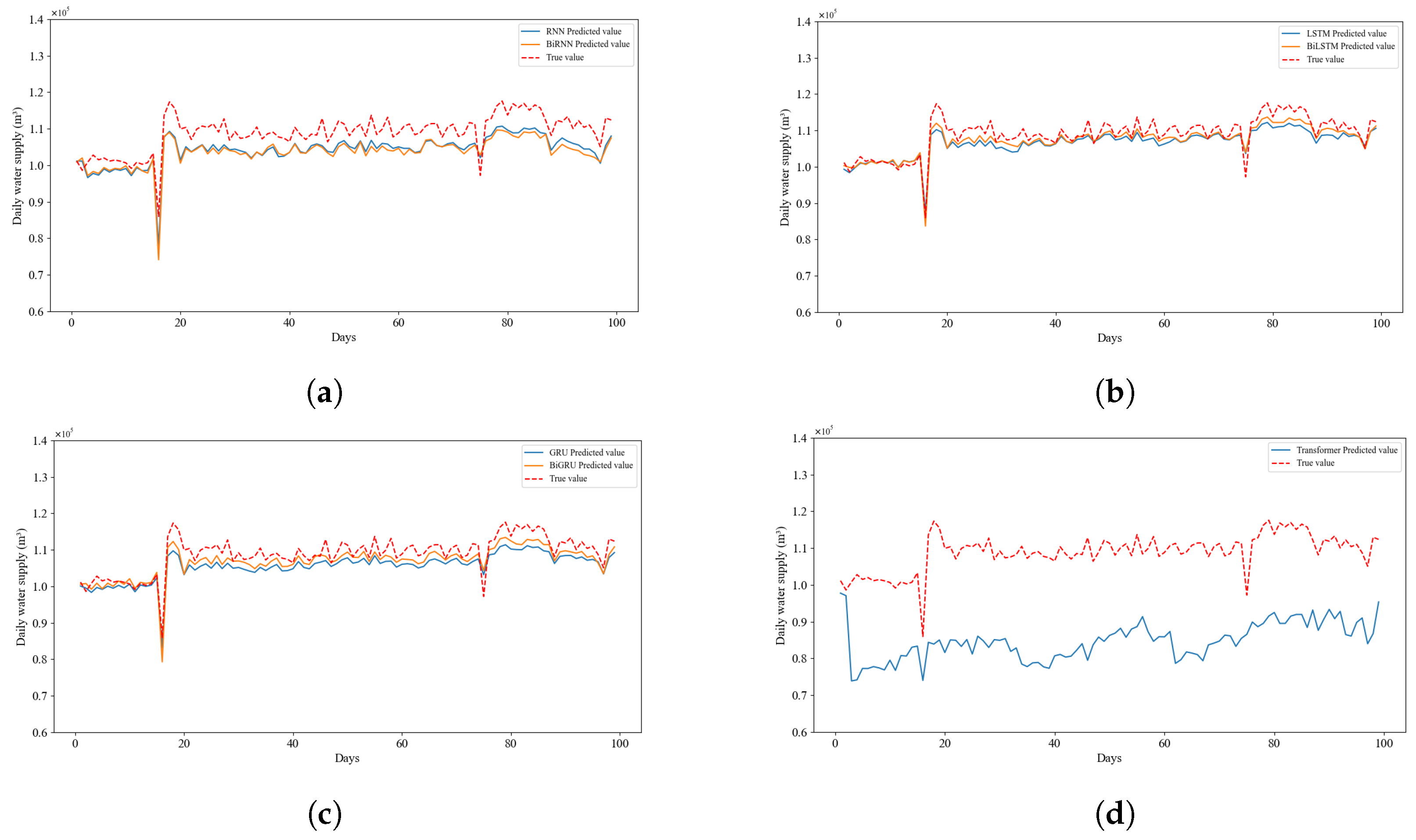
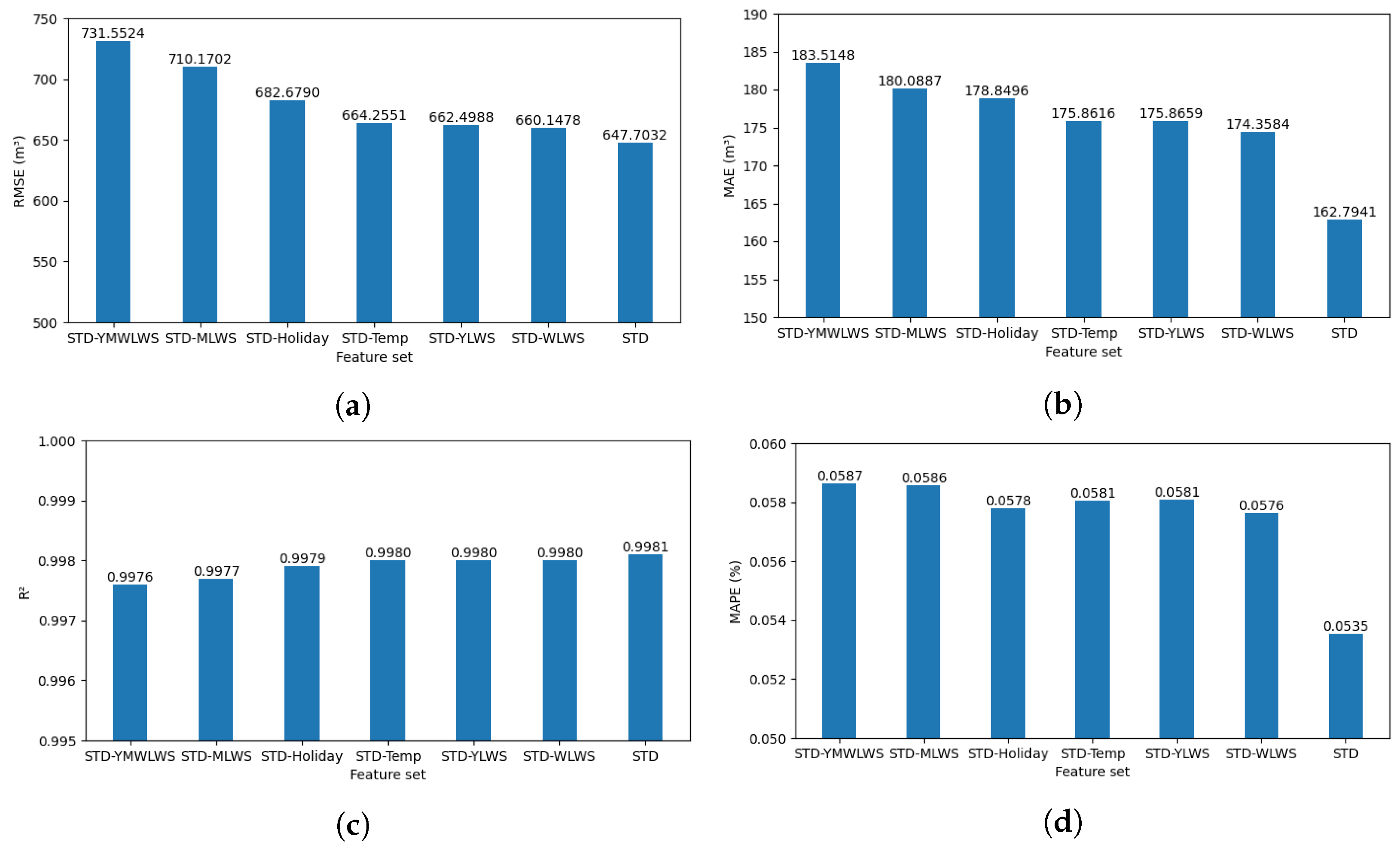
The above feature sets are used as inputs to the LSTM model, and the number of iterations of the LSTM model is set to 76 according to the Bayesian optimization results, which eliminates the overfitting phenomenon of the model and fixes the rest of the model hyperparameters. The performance metrics in Section 3.2 are also used to evaluate the models using different feature sets as inputs, and the results are shown in

Table 7. Performance of LSTM with different feature sets.

Metrics	STD- YMWLWS	STD- MLWS	STD- Holiday	STD- Temp	STD- YLWS	STD- WLWS	STD
RMSE (m3)	731.5524	710.1702	682.679	664.2551	662.4988	660.1478	647.7032
MAE (m3)	183.5148	180.0887	178.8496	175.8616	175.8659	174.3584	162.7941
MAPE	5.8651%	5.8587%	5.7799%	5.8067%	5.8074%	5.7638%	5.3530%
R2	0.9976	0.9977	0.9979	0.9980	0.9980	0.9980	0.9981

, while Figure 20 visualizes the performance metrics of the models. It is found that deleting any feature factor from the standard feature set results in a decrease in the model performance, where the model performance changes significantly when water supply with a 1-year lag, water supply with a 1-month lag, and water supply with a 1-week lag are deleted simultaneously, and the percentage error rises by 0.5121%.

The experiment indicates that the temporal multi-scale feature set introduced in this study is effective for predicting the water supply quantity at water plants. Each temporal multi-scale feature contributes to the model’s predictions to varying degrees, with the water supply quantity lagged by one month having a more substantial impact. Consequently, these features should be incorporated into the feature set to enhance the model’s predictive performance and its ability to generalize, thereby bolstering the water control and resource planning capabilities of the water plant.

4. Conclusions

This study was conducted with experiments targeting a specific water plant. By meticulously analyzing its historical water supply data and environmental factors, it innovatively proposes to construct a feature set by combining historical water supply data from the perspective of multiple time scales. The aim is to comprehensively consider various factors that influence the water supply volume and conduct a strict correlation analysis to explore the importance of features at different time scales for water supply volume prediction. The results show that the six models (except for the Transformer model) constructed based on this feature set can provide relatively accurate (with percentage errors all less than 7%) predictions of the water supply volume for the next 24 h for this water plant, helping the water plant to reasonably arrange water resource dispatching and ensure the stability of the water supply. Although this study is based on the data of a specific water plant, its research methods and achievements also have significant promotional value for other similar water plants. The ideas of selecting features with multiple time scales and applying deep learning models can offer useful references for water plants of the same type, helping them improve the accuracy of water supply volume prediction and optimize water resource management strategies.

Meanwhile, this study also has certain limitations. In terms of data application, although historical water supply data and some environmental factors have been utilized, there is still room for expanding the data dimension. Moreover, compared with large-scale datasets, the amount of data in this research is relatively limited and may not comprehensively cover all water supply change scenarios, which imposes certain constraints on the generalization ability of the model.

For future study work, on the one hand, we will further optimize the construction of feature sets. We will collect more extensive historical water supply data and relevant environmental factors, such as adding monitoring data like rainfall amounts and sunshine hours, and conduct in-depth analyses of the relationships between them and the water supply volume to build more comprehensive and effective feature sets. This will enhance the model’s ability to predict changes in the water supply volume under different environmental conditions. On the other hand, since existing research has shown that hybrid models may have advantages in water supply volume prediction, in the future, we will attempt to combine deep learning models with traditional statistical models or machine learning models to build hybrid models. By making full use of the strengths of each model, we can further improve the accuracy and stability of prediction and provide stronger support for the water supply management of water plants.