Estimating the Maximum Depth of Andean Lakes: A Comparative Analysis Using Machine Learning

Abstract

Multispectral modelling of 114 tropical Andean lakes in Southern Ecuador was implemented using observations of the maximum depth (Z_max). Five machine learning methods (MLMs), namely the multiple linear regression model (MLRM), generalised additive model (GAM), generalised linear model (GLM), multivariate adaptive regression splines (MARS), and random forest (RF), were applied on a LANDSAT 8 mosaic. Within the scope of a split-sample (SS) evaluation test, for each of the MLMs, a single model was developed for 70% (i.e., 80) of the studied lakes. Statistical measures and graphical inspection were used in the evaluation tests. An analysis of the absolute value of the model residuals (|res|) revealed that the MARS method outperformed the other MLMs. Nevertheless, a |res| > 10 m was observed for approximately 10% of the lakes. The worst predictions were produced by the GLM. These findings were confirmed in the model validation phase (SS test). With the exception of the GLM, the MLMs correctly predicted whether a lake was shallow or deep in more than 80% of the cases. In a more stringent multi-site (MS) test, the performance of the five Z_max models was assessed in predicting the bathymetry of 11,636 pixels that were not considered when fitting the models. Once more, MARS outperformed the other MLMs. However, a |res| > 10 m for 20% of the pixels was observed. Nevertheless, the quality of the predictions may still be regarded as acceptable for management purposes. Promising multispectral bathymetric predictions could be obtained, even with only a limited number of observations. The evaluation tests used in this pioneering study could be easily replicated elsewhere.

1. Introduction

Natural resources are fundamental for developing countries such as Ecuador. Hence, it is essential to have appropriate tools for scientifically/technically acquiring data to contribute to the better management of these resources. The generation of this information often requires significant financial resources, time, and/or physical effort. This is especially relevant in Ecuador, where the topography is highly variable [1] and there are extended areas where the accessibility is poor or almost non-existent, even from nearby populated cities (e.g., high mountain regions above 3000 m of elevation, the Amazonian forest, etc.). Cajas National Park (CNP) is only 20 km away from Cuenca, the third largest city in Ecuador, with approximately half a million inhabitants [2]. However, the generation of scientific knowledge about CNP requires important financial resources and physical effort [1,3,4], which could explain why there are still many under-investigated aspects of this valuable but extremely fragile ecosystem [1,5]. Hence, the use of alternative methods that significantly reduce these high temporal, financial, and physical costs, but still produce acceptable environmental information, is greatly needed.

The use of remote sensing data is likely to be a feasible option to produce the required technical information with lower costs. These data are successfully being used in different environmental assessments. Hence, the development of a robust method for the digital interpretation of satellite images and the use of geographic information systems (GISs) has the potential to provide highly useful products for the management and conservation of natural resources [6] within a much shorter timeframe and with significantly lower physical/financial costs than traditional methods.

In this regard, admissible hydromorphological information on tropical high-mountain lakes can play an important role in local and regional management, as lakes are fundamental for hydrological and biochemical cycles, storing a large proportion of surface freshwater and offering numerous valuable services within the ecosystem [7,8]. The mapping of the lake bathymetry is critical in understanding and characterising these ecosystems [3,9,10] to provide a foundation for their appropriate management and conservation [11].

Satellite-derived bathymetry (SDB) applications are conventionally based on the (empirical or physically based) identification of wavelength attenuation in the water column [12,13,14,15]. Commonly, these applications include a form of regression analysis (e.g., the generalised linear model—GLM) and/or principal component analysis (PCA) between field bathymetric observations (targets) and multispectral information. Different levels of accuracy have been achieved through the application of these methods [16]. More recent studies, registering better accuracy in many cases, are based on the use of empirical machine (or data) learning methods [17,18] to develop predictive models of the bathymetry in water environments. For example, Hassan and Nadaoka [10], Manessa et al. [19], Mabula et al. [20], and Xie et al. [21] applied supervised learning methods for SDB calculations, such as the GLM, random forest (RF), support vector machine (SVM), and multivariate adaptive regression splines (MARS), together with more traditional methods such as neural networks (NNs). Furthermore, other methods such as the multiple linear regression model (MLRM), generalised additive model (GAM), least square boosting (LSB) fitting algorithm, Gaussian process regression (GPR), decision tree regression, and K-neighbour regressors have been used for SDB calculations [19,22,23,24].

In particular, SDB applications have been carried out in shallow water environments such as coastal areas and the nearby shorelines of lakes [9,10,13,15,20,21,24,25,26]. However, few SDB studies have focused on deeper waters [9,25], although the SDB validation did include shallow water observations in some of these cases (e.g., Li, Gao, Zhao, and Tseng [9]). Furthermore, the few SDB studies on lakes have not simultaneously considered multiple lake domains; rather, they have focused on isolated lake environments.

The Cajas Massif (MzC), located in the southern Andes of Ecuador and encompassing CNP, has a large density of water bodies (more than 6000 across a surface area of approximately 9700 km²). CNP provides good-quality waters [5] that satisfy an important proportion of the diverse water demands of Cuenca City, and even of Ecuador, including water for drinking, industry, irrigation, and electricity generation. The management of these lakes is therefore focused on their ecological conservation; in this context, knowledge of the bathymetric parameters of the lakes is critical in understanding and characterising these ecosystems. It is also important to investigate the potential for the use of remotely sensed imagery for their management, including SDB studies that—unlike those commonly reported in the literature—simultaneously focus on several water bodies given the large number of lakes in the study area (many of which are deep).

Therefore, the main objective of the current research was to investigate the potential to derive bathymetric maximum depth (Z_max) information, which is useful for the (conservation) management of the tropical Andean lakes in Southern Ecuador, using remotely sensed imagery in a simultaneous multiple-lake framework. The specific research questions were the following: (i) Is it possible to delineate a methodology for the estimation of Z_max with acceptable accuracy from remote sensing imagery? (ii) Is it possible to estimate, with an acceptable rate of success, whether a lake is shallow or deep by using this methodology? (iii) Is it possible to define an evaluation protocol to effectively characterise the accuracy of the Z_max derived from remote sensing imagery? To the best of our knowledge, this is the first attempt to use remotely sensed imagery to characterise a key hydromorphological variable, i.e., Z_max, for multiple tropical high-mountain lakes, many of which are deep, using a single SDB model for several lakes and a small number of bathymetric observations. Both the use of a few bathymetric observations per lake (in this case, only a single observation) and the simultaneous modelling of all studied lakes with a single model reflect the lake management conditions that are usually observed in developing countries, where financial constraints prevent the detailed monitoring and modelling of lake districts.

2. Materials and Methods

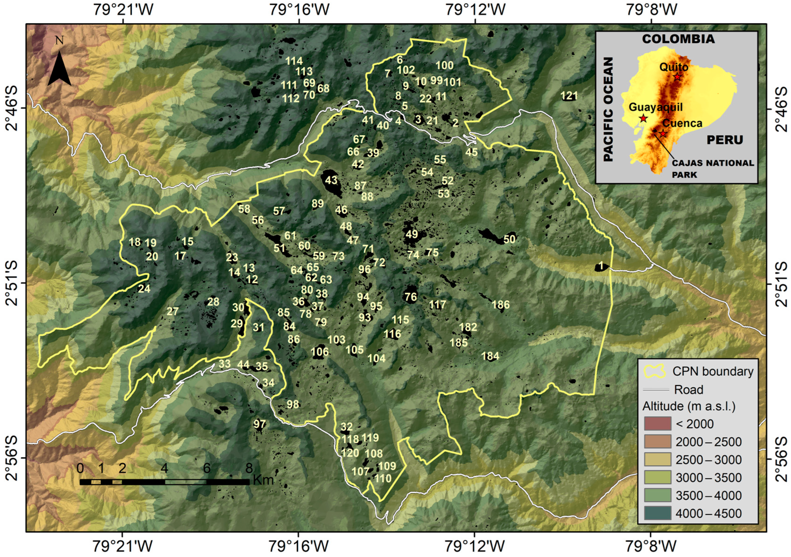
2.1. The Study Area

The study area was Cajas National Park (CNP; Figure 1), which belongs to the Cajas Massif (MzC) UNESCO Biosphere Reserve, located in the southern Andes of Ecuador. The surface of CNP amounts to approximately 285 km². It drains into the Pacific Ocean through the Jubones River basin and into the Atlantic Ocean through the Paute River basin and posterior (lower) Amazonian basins. CNP is the source of drinking water for nearly 60% of the population of Cuenca, which is the third largest city in Ecuador (approximately 600,000 inhabitants). The elevation of CNP (Figure 1) spans between 3150 and 4460 m above sea level (a.s.l.). The main soil units in the study region are Holocene Andosols and Histosols of volcanic origin [27]. The Pleistocene Tarqui volcanic bedrock is the main formation, which includes rhyolite, andesite, tuff, pyroclastics, and ignimbrites [28,29]. Herbaceous vegetation with the predominant presence of the Stipa and Calamagrostis genera covers approximately 90% of the total extent of CNP [30]. Only Polylepis spp. [31] are present at elevations higher than 3400 m a.s.l. A high-mountain forest (i.e., “bosque montano”) is present below the alpine lake’s lower elevation bound. The yearly precipitation ranges between 900 and 1600 mm, with contrasting seasons and large variation from year to year [32].

CNP (Figure 1) includes a large number of lentic systems of glacial origin [1,5]. In this work, one hundred and fourteen lakes (i.e., n_L = 114) were studied. Only one lake is situated below 3500 m a.s.l. (Figure 2a); two of them are located above 4300 m a.s.l. Most of them (i.e., 99) are deeper than 4 m (Figure 2b). With the exception of one of them, their surfaces are larger than half a hectare (Figure 2c); four of them cover surfaces greater than 46 ha. Their storage volumes also vary across a wide range (Figure 2d). These lakes are situated in the upper portion of the Paute River basin (Figure 3a); some of them are located outside the bounds of CNP (Figure 1 and Figure 3b).

2.2. Satellite Imagery

LANDSAT 8 (L8) Operational Land Imager (OLI) and Thermal Infrared Sensor (TIRS) images were used (Figure 3a). These were gathered from the website https://earthexplorer.usgs.gov/ (accessed on 9 March 2018) of the United States Geological Survey (USGS), which houses archives from the 2013 L8 project. LANDSAT images are subject to distortion from the sun, atmosphere, and topography; pre-processing minimises these distortions in the images [10,33]. Hence, the acquired Level-1T (L1T) images belonged to pad 10, row 62, and they had already undergone pre-processing with the following corrections: topographic (TOA), spectral, terrain accuracy, systematic terrain, and systematic geometric [34,35]. They were acquired on 20 November 2016, when the cloudiness in the study area was very low (Figure 3a). Only one scene was necessary to cover the whole study area (Figure 3a). Nine images, amounting to one per LANDSAT sensor band (B_m, with m = 1, 2,…, n_B = 9)—namely bands 01 to 07 (from the OLI sensor) and bands 10 and 11 (from the TIRS)—were used. Bands 08 (panchromatic) and 09 (for cloudiness studies) were discarded. The resolution of bands 01 to 07 was 30 m, while that for bands 10 and 11 was 100 m. The images were further cropped to a shorter extent (Figure 3b) to speed up the different calculation processes.

2.3. True Lake Bathymetry and Selection of Bathymetric Target Values

The lake bathymetry derived from the interpolation of detailed sonar survey data for the studied lakes was available [3], from which bathymetric target values (i.e., the maximum depth Z_max) for the current modelling were obtained. To limit the length of the present manuscript, only a brief description of the process used to generate the true bathymetry is given here. For further details, the reader is referred to Vázquez, Mosquera, and Hampel [3]. Surveying field campaigns [1] were carried out with the aid of an inflatable rubber boat (Navigator II, RTS, Hong Kong, China) and a sonar device (echo sounder, HumminbirdVR model 1198c SI, Eufaula, AL, USA) equipped with a GPS positioning system (Figure 4a). The distance between the surveyed bathymetric points was very small for small-surface lakes; moreover, for the larger lakes, it did not exceed 5 m [3]. Detailed field observations were used to model the bathymetry of the 114 studied lakes through an interpolation process that included the following steps [3]: (i) pre-processing of the bathymetric observations to correct any potential anomalies that arose during the surveying campaigns (e.g., incorrect georeferencing or data outliers, etc.); (ii) processing of the bathymetric observations to ensure the correct format; (iii) random splitting of the available observations into training and validation data sets (split-sample (SS) test); (iv) application of eleven interpolation algorithms to the training data set to select the best algorithm (Figure 4a); (v) validation of the selected algorithm using the respective validation data set (SS test); and (vi) application of the selected algorithm (Kriging Standard [36]) to obtain the true bathymetry of each of the 114 study lakes (Figure 4a). For the (automatic) interpolation process, SURFER version 16 was used. Data handling, including the random splitting of the available observations into training and validation data sets (SS test) and the statistical assessment of the performance of the interpolation algorithms (Figure 4a), was conducted with task-specific subroutines programmed with the Practical Extraction and Reporting Language (PERL).

2.4. Selection of Bathymetric Targets (Ztl,j) and Multispectral Observations (Btl,j) of the Different LANDSAT 8 (L8) Bands

Once the bathymetric surfaces of the study lakes were produced, a target bathymetric value (Zt_l,j), i.e., Z_max in the current case, was selected for each of the 114 lakes (Figure 4b). Then, the geographically corresponding multispectral values (Bt_l,j) were obtained for each of the L8 sensor bands. Nine digital levels (DLs) for bands 01, 02, 03, 04, 05, 06, 07, 10, and 11 of L8 level L1T were used. Thus, data matrix A (Figure 4b), with 114 entries (one per study lake) containing the Zt_l,j of a given lake and its respective (nine) multispectral values (i.e., Bt_l,j; Figure 4b), was built for further use during the multispectral bathymetric modelling. Both Zt_l,j and Bt_l,j were selected with the aid of SURFER, ArcGIS version 10.3, and a task-specific PERL subroutine.

2.5. Modelling the Lake’s Maximum Depth (Z_max) Using Zt_l,j and Bt_l,j

2.5.1. Splitting the Total Observations into Training and Validation Data Sets (Split-Sample Test)

Data matrix A of the total bathymetric and multispectral observations (Figure 4b) was randomly split (SS test) into sub-matrices B (training) and C (validation) of sizes (f_L) (nt_j × n_L) × (1 + n_B) and (1 − f_L) (nt_j × n_L) × (1 + n_B), respectively; this included the number of bathymetric targets for lake j, nt_j = 1 (i.e., Z_max), for every study lake. The data splitting fraction for training (f_L) was fixed in this study at 0.7. In other words, 70% of the studied lakes (i.e., 80) were randomly selected for the training phase of the SS test (i.e., for the fitting of the Z_max models). The data for the remaining 30% of the lakes (i.e., 34) were used in the validation phase. Cluster sampling was used to ensure that 70% of the shallow lakes (i.e., having Z_max < 4 m) and deep lakes (i.e., Z_max ≥ 4 m) were randomly selected for the training data set.

2.5.2. Modelling Methods

Five different machine learning methods (MLMs) for the estimation of Z_max as a function of the bathymetric and multispectral observations were used, namely (a) the multiple linear regression model (MLRM), (b) the generalised additive model (GAM) using spline functions, (c) the generalised linear model (GLM), (d) multivariate adaptive regression splines (MARS), and (e) random forest (RF). These MLMs were chosen to inspect the performance of both linear and non-linear supervised learning algorithms, given that several recent bathymetric studies have used these with varying success (e.g., [10,13,19,34,37,38]). Although the use of linear models in the context of problems, such as the current one, that are inherently non-linear requires us to explicitly address these non-linearities, these methods were applied blindly. R^® version 4.1.0 was used for their application. GIS operations, including map algebra, statistical analyses, data format conversion, and cartography preparation, were carried out with ArcGIS version 10.0, Terrset version 18, and SURFER version 16. In the following, only a brief description of each method is provided.

It is important to note that, contrasting other studies (e.g., [38,39,40,41]) that mainly address shallow waters, no spectral band ratios were used in the current modelling. In particular, given that most of the study lakes were deep, and for the sake of simplicity and uniformity, absolute optical information was used. In this research, it was assumed that the bottom surface of a given lake was homogenous and the respective water column was uniform across the whole lake [10,41]. Furthermore, no selection of the most relevant independent variables (i.e., spectral bands) was carried out; rather, all of the bands were used, aiming for a fairer comparison of the bathymetric predictions produced by the different MLMs. When applying the MLMs, Z_max was the dependent variable, and the observations of the nine L8 sensor bands (X_m) were the independent ones.

The MLRM is a well-known multi-layer method that is applied in remotely sensed empirical modelling [42], including the bathymetry of water bodies [19,43]. The built-in multiple linear regression lm( ) function of R^® (version 5.1.0) was used for its implementation.

The GLM is based on a linear combination of non-random X variables with a random dependent variable, namely Z_max ([38,39]). The GLM has typically been used to model shallow lakes [40]; nevertheless, in this study, it was also applied to model the bathymetry of deep lakes (Figure 2b). We chose to use the quasi-Poisson error distribution, which assumes that the variance of the data is the respective mean multiplied by a dispersion parameter (α). This is normally suitable for data that are over-dispersed, i.e., when the data variance exceeds the mean [44]. A negative binomial distribution [45], which is a generalisation of the Poisson distribution, is an alternative error distribution used to handle over-dispersed data; it was also tested in the current research. The GLM was implemented through the glm( ) function from the base R^® stats package, version 4.1.0. The fitting process was based on the least-squares method.

The more flexible GAM, as an extension to the traditional GLM, enables researchers to account for non-linear relationships through non-parametric smoothing functions applied to the predictor variables [37,46]. The GAM was implemented through the gam( ) function of the R^® package “GAM” version 1.22-5. Gaussian distribution was chosen, with the link function “identity”. The iteratively reweighted least-squares (IWLS) method was used to fit the parametric part of the model.

MARS is a multivariate, piecewise, non-parametric linear regression technique. It involves dividing the training data set into regions and then generating a linear regression equation for each of them [22]; these are connected to each other through “nodes” or “knots” [47,48,49,50]. MARS was implemented through the R^® package “Earth” version 5.3.4.

RF is a non-linear ensemble learning method that belongs to the decision tree automatic learning family and is suitable for regression, classification, and prediction. It is formed through the growth of trees depending on a random vector [19,34]. This produces a series of subsets of the entire data set, among which information is exchanged. Finally, all the decision trees are aggregated to produce a single forest. The version utilised herein relied on the root mean square error (RMSE) criterion, defined later in the text; this was used to calculate the quality of a subset division, aiming at minimising the error variance. It has been successfully used in several SDB studies [19,20,21,24,34,38] and other remote sensing studies [46]. The R^® package “randomForest” version 4.7−1.2 was used for its implementation.

2.5.3. Statistics for the Evaluation of the Performance of the Z_max Multispectral Models

Model performance indices were used to characterise the quality of the empirical algorithms used to simulate Z_max. This was conducted for each of the considered empirical algorithms and for both the training and validation data sets (within the scope of a traditional split-sample test, as discussed later in the text). This involved developing appropriate subroutines in TerrSet^®, ArcGIS^®, and R^®, as well as programming task-specific subroutines with PERL^®, to carry out the assessment automatically. In general, GNUPLOT^® and Excel^® were used for plotting purposes.

These performance indices were based on residuals (res_q [L]), i.e., the difference between the q-th bathymetric target (Zt_q [L]) and the respective prediction (Zp_q [L]), and were selected to measure [51] (i) the average (model) systematic error, (ii) the average combined systematic and random error, and (iii) the correlation among the bathymetric target data and predictions. Hereafter, the mean absolute error (MAE) [L], defined as the average of the absolute value of the residuals (|res_q| [L]), was used as a measure of the average (systematic) error of each of the multispectral models. This was used as it prevents residuals of the opposite sign cancelling each other out (which produces a false impression of model accuracy, as in the case of the BIAS index, although this has been used in past SDB studies [21]) [52]. Its optimal value is zero, and it has also been used in past SDB studies [10,20,21,24,38].

The efficiency coefficient (EF₂) [−], also known as the Nash–Sutcliffe coefficient [53], was used as a dimensionless measure of the total (combined systematic and random) average model error. It is defined as a function of the square of the residuals:

$$\mathrm{E}{\mathrm{F}}_2=1-{\displaystyle \frac{{\displaystyle \sum _{\mathrm{q}=1}^{\mathrm{n}\mathrm{t}}{\left(\mathrm{z}{\mathrm{t}}_{\mathrm{q}}-\mathrm{z}{\mathrm{p}}_{\mathrm{q}}\right)}^2}}{{\displaystyle \sum _{\mathrm{q}=1}^{\mathrm{n}\mathrm{t}}{\left(\mathrm{z}{\mathrm{t}}_{\mathrm{q}}-\overline{\mathrm{z}\mathrm{t}}\right)}^2}}}$$

(1)

where $\overline{\mathrm{z}\mathrm{t}}$ [L] is the average of the bathymetric target observations used in the model evaluation, and nt [−] is the total number of bathymetric target observations considered in the model evaluation. In this expression, the composed sub-index “l,j” is replaced by the sub-index “q” because once the geographical points for the evaluation of the bathymetric predictions have been defined, the evaluation of EF₂ becomes a simpler, one-dimensional expression. The optimal value of EF₂ is 1.0, and the feasible range of variation is −∞ < EF₂ ≤ 1.0. Negative values of EF₂ indicate that the model performs poorly in comparison to using $\overline{\mathrm{z}\mathrm{t}}$ as a predictive model [53,54]. A literature review indicated that it has not yet been used in the context of SDB.

Further, the root mean square error (RMSE) [L], defined as the square root of the average summation of the square of the residuals, has been widely used—in remote sensing in general [37,47] and in SDB research in particular [10,20,21,24,34,39,40,55]—for the characterisation of the average systematic error. Similarly to the MAE, it is expressed in the same units as the bathymetry (although in some studies, its units are not acknowledged, e.g., [39]), and its optimal value is also zero. However, the RMSE index is directly correlated with the EF₂ coefficient [52], implying that both of them measure essentially the same information about the model residuals: the total (combined systematic and random) average model error. Nevertheless, it was also used herein (together with the EF₂) to enable a comparison with past research [19,20,21,24,38].

The R² (or r²) coefficient of determination, or the square of the Pearson’s type correlation coefficient (R or r), is also commonly reported for the characterisation of the performance of simulation models [20,21,24,37,47]. Nevertheless, it presents several shortcomings in this context, including its oversensitivity to the prediction of peak values [53]. This is also one of the limitations of the EF₂ index, although to a lesser extent than for the R². Hence, R² was used in this study, but only to characterise the correlation between the observed and predicted bathymetric data and for a direct comparison with previously published SDB and water level modelling studies [12,19,20,21,24,38,39,55].

An alternative model performance measure to the EF₂ is Kling–Gupta efficiency (KGE) [−], which is widely used in hydrological modelling [56,57]. This was also used in this research, as in past SDB studies [38]. It has the same range of variation as the EF₂ and is calculated through the following expression:

$$\mathrm{K}\mathrm{G}\mathrm{E}=1-\sqrt{{\left(\mathrm{R}-1\right)}^2+{\left({\displaystyle \frac{{\mu }_{\mathrm{s}\mathrm{i}\mathrm{m}}}{\overline{\mathrm{z}\mathrm{t}}}}-1\right)}^2+{\left({\displaystyle \frac{{\sigma }_{\mathrm{s}\mathrm{i}\mathrm{m}}}{{\sigma }_{\mathrm{o}\mathrm{b}\mathrm{s}}}}-1\right)}^2}$$

(2)

where μ_sim [L] is the mean of the bathymetric predictions, and σ_obs [L] and σ_sim [L] are the standard deviations of the (observed) bathymetric targets and bathymetric predictions, respectively.

The above-depicted indices use a single value to characterise the multispectral model’s performance in simulating the nt bathymetric spots. When inspecting the spatial and frequency distributions of the residuals, for every pixel of interest, |res_q|, as well as the dimensionless absolute relative error (|re_q| = |res_q|/ Zt_q), was considered. Hence, the spatial distribution of the residuals was assessed through the use of GIS software (ArcGIS^® and TerrSet^®), with its visual and arithmetic capabilities. Meanwhile, the frequency distribution of the residuals was assessed through the use of empirical exceedance probability distribution curves, which were defined on the basis of the Weibull plotting position of a quantile method [58].

2.5.4. Test for the Evaluation of the Performance of the Z_max Multispectral Models

A traditional split-sample (SS) test was initially carried out. Thereafter, a single bathymetric multispectral model was developed using the training data set (80 lakes) for each of the MLMs. Six multispectral models were built. Each model considered all 80 values of Z_max. The assessment of the quality of the predictions was carried out by inspecting the evolution of the curves of the empirical probability of the exceedance of |res| and |re|, as well as the distribution of the 80 pairs of observed and predicted Z_max values through scatter plots. The model performance statistics were also evaluated for this purpose. The SS test included an examination of the performance of the models using the validation data set (34 lakes) for each of the MLMs. The main objective of this SS model performance evaluation was to select the most convenient MLM for the current multispectral modelling of the SDB.

Within the scope of this test, the performance of the GLM involved different parametrisations as a function of the type of error distribution (either quasi-Poisson or negative binomial) and the values adopted by the dispersion parameter (α) of the negative binomial distribution. This analysis was also implemented as it is known that GLMs cannot cope with multi-collinearity among the independent variables, which was possible within the multispectral information considered in this study. Nevertheless, it is emphasised that a variable selection procedure to identify the most important and simultaneously uncorrelated L8 bands was beyond the scope of this study.

A second model performance evaluation was carried out to address the management requirement for knowledge of whether a given lake is either shallow or deep. This was achieved by examining the proportion of correct lake classifications as either shallow or deep for each of the five Z_max multispectral models. For this, the bathymetric threshold of 4 m, determined in prior research [1], was used, so that lakes were considered shallow when Z_max < 4 m and deep when Z_max ≥ 4 m, either for observed or predicted conditions. This test is independent of the SS test as it does not deal with the training of the implemented bathymetric models; it is entirely focused on model performance evaluation. Therefore, it was implemented considering three sub-analyses, namely global (using all of the 114 study lakes), shallow (using only the 15 shallow lakes), and deep (considering the 99 deep lakes).

A final model performance evaluation, namely a multi-site (MS) test [51,52], was carried out to address the management requirement for the estimation of the bathymetric properties of non-instrumented remote lake districts. In this test, each of the six Z_max multispectral models was required to predict the bathymetry of (multi-site) lake pixels situated at different locations compared to the Z_max positions that were considered in the SS test. Consequently, it was also independent of the SS test. Thus, pixels belonging to each of the 114 study lakes were considered in this MS test. In total, each of the multispectral models was required to predict the bathymetry of 11,636 pixels.

3. Results

Modelling the Lake’s Maximum Depth (Z_max) Based on the Use of Bathymetric Targets and Multispectral Observations

The Z_max predictions of the different inspected MLMs for the studied lakes were evaluated against the respective Z_max target values for both the training and validation phases of the modelling in the split-sample (SS) test. Figure 5 shows the empirical cumulative frequency distributions of both (i) the absolute values of the residuals (|res|) among the observed and modelled Z_max and (ii) the absolute values of the relative errors (|re|) among the observed and modelled Z_max. The ranges of |res| and |re| used in the figure were chosen subjectively with the intention of presenting a clear picture of the general performance of each MLM; higher values than the plotted ranges were obtained for some of the deeper modelled lakes. The empirical distributions depict the estimated exceedance probability of occurrence. The figure illustrates that for either |res| or |re|, in the SS model training phase, the best performance was achieved with the MARS method. Furthermore, the GLM (using quasi-Poisson distribution) produced Z_max estimates that were far less accurate than those of the other applied methods. Although not depicted herein, these results were also confirmed in the SS model validation phase.

Furthermore, Figure 6 shows the scatter plots of the observed (Depth_obs) versus the modelled (Depth_sim) Z_max as a function of the MLM. The plots also include the 1:1 diagonal line. Each plot corresponds to one of the applied MLMs and contains the respective values for the model performance statistics. Each dot relates to one of the 80 (i.e., 70%) studied lakes randomly selected for the SS training phase. Each of the model performance statistics was calculated using these 80 pairs of Depth_obs and Depth_sim values.

The scatter plots confirm that in the training phase of the modelling, the MARS method produced the best estimates of Z_max for the 80 studied lakes, and the GLM (with quasi-Poisson distribution) produced the least accurate Z_max predictions. These findings were confirmed in the validation phase (Figure 7) of the SS test using the data of the remaining 34 lakes that were not considered in the training phase.

Figure 8a,b illustrate the results of the assessment of the effects in the performance of the GLM when using the negative binomial error distribution rather than the quasi-Poisson distribution. Besides the distributions of the |res| among the observed and modelled Z_max (Figure 8a), the results include the distributions of the |re| among the observed and modelled Z_max (Figure 8b). This figure depicts the distributions of six GLM-based multispectral bathymetric models, namely GLM₁, which used the quasi-Poisson distribution; GLM₂, which used the negative binomial distribution with the automatic optimisation of α; and GLM₃ to GLM₆, which used the negative binomial distribution with different explicit α-values in the range of 2.0 to 6.4 (optimal value). The depicted results were obtained for the SS training phase. These plots indicate that there were almost no differences among the respective predictions of the GLM-based models.

Table 1. The proportion of shallow/deep lake classifications correctly predicted by the maximum lake depth (Z_max) multispectral models based on the applied machine learning methods: MLRM = multiple linear regression model; GAM = generalised additive model; GLM = generalised linear model; MARS = multivariate adaptive regression splines; RF = random forest. The “global” analysis considered both shallow and deep lakes, the “shallow” analysis considered only shallow lakes, and the “deep” analysis considered only deep lakes. Numbers in bold depict either a perfect (1.0) or completely incorrect (0.0) predicting capability of the applied machine learning methods.

		Machine Learning Method
Analysis	Number of Lakes	MLRM	GAM	GLM	MARS	RF
Global	114	0.84	0.85	0.14	0.88	0.87
Shallow	15	0.40	0.40	1.00	0.33	0.00
Deep	99	0.91	0.92	0.01	0.96	1.00

lists the results of the second model performance evaluation, which assessed how well the Z_max multispectral models could distinguish between shallow and deep lakes. For the global analysis, proportions larger than 80% were observed for all methods except the GLM. The latter method had a successful classification rate of almost 0% for deep lakes; however, it had a 100% success rate for shallow lakes. The remaining methods performed well for deeper lakes, particularly RF. These results are of particular relevance for management. It must be emphasised that this evaluation test is not focused on the bathymetric prediction accuracy but rather on the ability of the bathymetric model to predict whether a lake is deep or shallow.

With respect to the multi-site (MS) evaluation of the bathymetric predictions produced by the five multispectral Z_max models, some negative bathymetric values were output by all of the applied MLMs except RF. In the case of MARS, approximately 1.9% of the total pixels (i.e., 11,636) were associated with negative bathymetric predictions. For instance, Figure 9a depicts the concentration of these negative-value pixels (predicted using MARS) in lakes located in the northern region of the study area (Figure 2b), outside the boundary of CNP. This situation is representative of what was observed for other lakes, where negative-value pixels were also predicted using MARS; these pixels tended to occur by the littorals, i.e., by the boundaries between the ground surface and the (lake) water extent. Furthermore, this issue tended to occur mainly for small-surface lakes, albeit with some exceptions.

The products of other MLMs, such as the GAM (Figure 9b), also produced negative-value pixels near the littorals of the studied lakes, although with a higher density in smaller-surface lakes. For the MARS bathymetric product, given the small proportion (i.e., 1.9%) of negative-value pixels, and considering that these mainly occurred at the littorals of the lakes (Figure 9a), we decided to eliminate these negative-value pixels from the MS evaluation. Thus, for a given region of the study area, Figure 9c illustrates the resulting spatial distribution of the predicted bathymetry from the MARS multispectral Z_max model. Furthermore, for the same region, Figure 9d depicts the respective distributions of pixels with |res| < 20 m.

The MS evaluation test was also carried out by calculating the empirical exceedance distributions of |res| and |re| (Figure 10). The MARS method appeared to perform better than the other methods, although only marginally in certain regions within the range of variation of |res|. Herein, for |res| > 18 m, the Z_max predictions of the GLM were the least accurate; however, for |res| ≤ 18 m, this was not the case. Figure 11 shows the respective scatter plots of the observed (Depth_obs) and simulated (Depth_sim) lake depths as a function of the MLMs. Each dot corresponds to a given pixel considered in the context of the MS model performance evaluation, and each of the model performance statistics was calculated using all 11,636 pairs of Depth_obs and Depth_sim values. Although the scatter of the data is significantly greater than that depicted in Figure 7 (SS test), the plots in this figure suggest that the MARS method produced the best bathymetric estimates and that the GLM method (with the quasi-Poisson distribution) produced the least accurate MS bathymetric predictions (using the Z_max multispectral models).

4. Discussion

Most previous studies have focused on the multispectral modelling of the bathymetry of shallow coastal shores or the littorals of shallow and relatively flat lakes located at lower elevations (e.g., Hassan and Nadaoka [10]; Li, Knapp, Lyons, Roelfsema, Phinn, Schill, and Asner [11]; Mabula, Kisanga, and Pamba [20]; and Yunus, Dou, Song, and Avtar [34]). In addition, previous studies have focused on single water environments or, at most, a few water bodies distributed across a narrow geographical domain; an independent multispectral bathymetric model was then fitted for each of the studied water bodies [10,11,34]. The present study differs from past research as it is one of the first attempts to model the bathymetric features of multiple tropical water bodies located within the broad geographical domain of the Andean highlands. Here, 114 water bodies, distributed across a moderately wide geographical domain (Figure 1 and Figure 2) and covering a large spectrum of different bathymetric, geomorphological, and even functional conditions [1,4,5], were studied. A single multispectral Z_max model for 70% (i.e., 80) of the 114 different study sites was developed, which is a particularly notable difference with respect to past research; however, there are likely to be considerable constraints in applying a single model to predict the bathymetry for such a large number of different water bodies with a comparable level of accuracy to that achieved in previous research.

In the split-sample (SS) evaluation test, a comparison of the 80 Z_max predictions with the respective true bathymetric data in the form of the exceedance (empirical) probability distributions of |res| and |re| (Figure 5) indicated that the MARS method significantly outperformed the other MLMs. The analysis also showed that three methods, namely the MLRM, GAM, and RF, produced very similar Z_max predictions, but these were less accurate than the ones produced with MARS. This differs from what was reported by Hassan and Nadaoka [10]. In their case, the RF method performed better than MARS, although their study differed significantly from the present one as they considered three modelling locations; these were coastal and lake regions that were relatively flat and shallow, and they developed individual models for each of these sites. Our results also differ from those of Yunus, Dou, Song, and Avtar [34], who found that RF performed very well, albeit only up to depths of 30 m. In the current case, RF did not only perform poorly compared to MARS but also failed to perform better than the GAM and MLRM (Figure 5). These outcomes differ from the results of Manessa, Kanno, Sekine, Haidar, Yamamoto, Imai, and Higuchi [19], who observed a considerably better performance of RF as compared to the MLRM. These findings support the idea that MLMs should not be selected at random; rather, it is necessary to carry out a selective analysis considering the different (physical) characteristics of the study sites, the locally available observations, and, most importantly, the available multispectral data, as was performed in this study and as also outlined by Mabula, Kisanga, and Pamba [20].

The SS analysis also indicated that the GLM always generated the worst Z_max predictions, as clearly represented by the nearly vertical |re| curve in Figure 5b. Nevertheless, the |res| curve for the MARS method (Figure 5) also illustrates that important residual values—for example, greater than 6 m—were observed for several of the studied lakes (approximately 40%). Moreover, |res| values higher than 10 m were obtained for approximately 10% of the lakes (the deeper ones). Although these |res| values might seem higher than those reported in past studies (e.g., Hassan and Nadaoka [10]; Li, Knapp, Lyons, Roelfsema, Phinn, Schill, and Asner [11]; Mabula, Kisanga, and Pamba [20]; Xie, Chen, Zhang, and Pan [21]; and Yunus, Dou, Song, and Avtar [34]), it should be noted that in these studies, (i) only shallow bathymetries were modelled, whereas the current study also included significantly deeper conditions, and (ii) an individual bathymetric model was developed for each modelled water body. In contrast, here, a single model was defined for all 80 different lakes considered in the SS training phase.

When evaluating the performance of the applied MLMs through the use of the performance statistics, namely the MAE, EF₂, KGE, R², and RMSE, as well as the visual inspection of the shapes of the calibration scatter plots (Figure 6), the above trends were confirmed. In particular, they highlighted (i) the remarkable ability of MARS to predict lower, medium, and higher Z_max values; (ii) the prediction problems associated with the MLRM, GAM, and RF, which over-predicted lower Z_max values and under-predicted higher values; and (iii) the lack of prediction capabilities of the GLM, as it systematically under-predicted all of the Z_max values. Although both the MLRM and GLM have intrinsic linear features (i.e., they are linear supervised learning algorithms), the better performance of the MLRM should be noted. The above findings were confirmed by the SS evaluation test in the model validation phase (Figure 7).

The lower prediction capabilities observed for the GLM contrast with what is commonly reported in the literature. The GLM has performed acceptably not only in SDB studies [40] but also within the scope of other remote sensing applications, where GLMs have even outperformed non-linear MLMs such as RF [46]. The lower GLM performance observed here seems to be independent of the error distribution being considered in the method, as suggested by Figure 8a,b. This figure shows that the use of either a quasi-Poisson distribution [44] or a negative binomial distribution [45,46] yields an equivalent performance, even when applying markedly different parameterisations. Overall, these results confirm the important intrinsic limitations of GLM methods in predicting the bathymetric features of deeper lakes. This is in line with Elshazly, Elshemy, Zeidan, and Armanuos [40], who recommend the GLM particularly for shallow lakes.

The second model evaluation test considered how well the Z_max multispectral models could predict shallow and deep lakes. This indicated that in general and for most of the MLMs, the proportions of correct lake classifications were high. An exception was the GLM, which yielded perfect predictions for shallow lakes but could not produce accurate predictions for deep lakes. These results are in line with the work of Elshazly, Elshemy, Zeidan, and Armanuos [40] regarding the GLM method. Most of the applied MLMs yielded successful predictions for deep lakes (Table 1). These results are particularly relevant for the management of lake districts. Regardless of the precision of the respective bathymetric multispectral models, even those based on very few bathymetric observations, some of the applied MLMs may discretise well between shallow and deep lakes.

To the best of our knowledge, the third model evaluation test, namely the multi-site (MS) test, has rarely been carried out in SDB research. Our analysis revealed that negative-value pixels were obtained (Figure 9a,b) for some of the MLMs, including MARS. These were mainly located by the littorals of small-surface lakes, i.e., at the boundaries between the ground and water. In these areas, the MLMs might have experienced problems in distinguishing between spectral information from the water and the surrounding ground. In the case of MARS, the MS test revealed, for every studied lake, a strong consistency in the depth distribution, with shallow depths by the littorals and deeper depths by the central portions of the lakes. The respective scatter plots (Figure 11) indicated that MARS also outperformed the other MLMs within the scope of this MS test, despite the fact that the models were fitted only considering the Z_max data. Nevertheless, significant |res| values were recorded when applying MARS (Figure 9d), although a large proportion of the pixels (approximately 90%) had |res| values < 20 m. Furthermore, it should be noted that the RMSE value (11.9 m) of the MARS predictions, achieved within the scope of this test, is similar to those reported in previous SDB studies (e.g., Abdul Gafoor, Al-Shehhi, Cho, and Ghedira [39]); however, they modelled significantly shallower bathymetries under less demanding conditions in terms of the number of modelled study sites and the bathymetric observations included in the modelling process compared to the present research. The MS test confirmed that the GLM method produced the worst bathymetric predictions.

As the MS test evaluated the performance of the (Z_max) multispectral models in predicting the bathymetry of pixels that were not considered in the (SS) model training phase, it required the Z_max models to predict beyond the data limits that were considered for their fitting. However, for each of the applied MLMs, a single model was fitted to encompass the Z_max values of all 80 different water bodies. Thus, considering the broad range of variation in the observed Z_max (i.e., [1.6, 75.8] m), it is likely that for the MARS method, this single model had the ability to predict a similarly broad spectrum of bathymetric variability. The outcome might be different for other local conditions—for instance, in the case of more uniform variation in Z_max (or any other bathymetric feature). Therefore, we emphasise the need to carry out local analyses, similar to those performed herein (and as highlighted, for instance, by Mabula, Kisanga, and Pamba [20]), before adopting a bathymetric model for management purposes.

This study devised a single multispectral bathymetric model for multiple study lakes based on the consideration of a limited number of bathymetric observations (one per lake) and after the comprehensive application of five different MLMs and three model performance evaluation tests. The evaluation tests suggested that for the chosen study site, the local conditions, and the available multispectral data, the best-performing MLMs produced more reliable models for deeper lakes than for shallow ones.

The study lakes are located within a national park (CNP). Therefore, there are no navigation issues associated with the ecosystem services of the study lakes. Therefore, the present findings have no implications for transportation ecology. Rather, the lakes’ ecological management focuses on their conservation, including that of their surrounding landscapes, because CNP provides good-quality water [5] that satisfies a large number of diverse water demands, including for drinking, industrial purposes, irrigation, and electricity generation. Thus, they contribute to the sustainable development of the city of Cuenca and even of Ecuador (in terms of satisfying the hydroelectricity generation quota). Hereafter, knowledge of bathymetry-related parameters such as Z_max will be fundamental in understanding, for example, the ecological functioning of these lakes [1,3] and, in turn, for their appropriate conservation and management. Nevertheless, the different methods and approaches used in this study could be applied at other latitudes where navigation and other uses must be ecologically managed within the framework of sustainable development. Knowledge of these bathymetric parameters would also be essential in these cases.

The main limitation of the current study is the significant residuals that were observed for certain evaluated lakes/pixels as compared to published results, particularly for deeper lakes. Nevertheless, as already stated, this study differs from past research in some key aspects, which implies that its results cannot be directly compared to other published findings. Despite this, future work aimed at improving the modelling performance should be focused on the following: assessing the effects of using spectral band ratios; considering alternative satellite products with finer resolutions (and similar spectral information), which would involve a scalability assessment [26]; and identifying the most significant spectral information for modelling, etc.

Furthermore, the single model that was developed in this study could be applied to diverse data sets for lakes across the Andean region of Ecuador in order to assess its generalisability and transferability to these locations. A related generalisability and transferability assessment within the current study area could involve developing more detailed SDB models of representative lakes—for instance, for shallow, average, and deep conditions—and applying them to the data of other lakes that share similar conditions. These analyses could be useful for conservational or management purposes.

5. Conclusions

Five different machine learning methods (MLMs) were applied to a LANDSAT 8 mosaic for the bathymetric modelling of 114 Andean tropical lakes in Southern Ecuador, using a single observation per lake, namely the maximum depth (Z_max). The performance of these five models was assessed through three different model evaluation tests that analysed the models’ bathymetric residuals. Both the traditional split-sample (SS) test and the multi-site (MS) test— that inspected the performance of each of the five Z_max models for pixels (i.e., 11,636) that were not considered in the training phase of the SS test—revealed that the multivariate adaptive regression splines (MARS)-based model outperformed the models resulting from the other methods, including the renowned random forest (RF) method. Despite the use of dissimilar error distributions, the worst predictions were produced by the generalised linear model (GLM), particularly for deeper lakes. Furthermore, all of the applied methods, with the exception of the GLM, yielded correct predictions in more than 80% of the cases concerning whether a lake was shallow or deep. The GLM yielded perfect predictions for shallow lakes, while it could not produce predictions for deep lakes. However, even for the MARS method, important residual values were observed, i.e., depending on the model performance evaluation test, |res| > 6 m for approximately 50% of the inspected pixels and |res| > 10 m for approximately 20% of the pixels (the deeper ones). Despite this, the quality of the predictions could be considered acceptable and useful for management purposes, particularly considering the convenience of using a single bathymetric model to manage 114 lakes rather than developing a model for each lake. The results of this pioneering study indicate that it is important to carry out different model evaluation tests, since the application of the same modelling methods may produce results that differ from those obtained in previous research owing to the prevailing local conditions. The tests used herein proved to be highly useful in addressing the holistic performance of the developed models; they can be easily replicated, independently of the geographical location. Another conclusion is that the remote sensing-based modelling of (multiple) lakes’ bathymetry with relatively few observations might be feasible and sufficiently accurate for management purposes. This is particularly relevant for the Andean lake districts, which are typically remote, similarly to the site analysed in the present study.

References

1. Mosquera, P.V.; Hampel, H.; Vázquez, R.F.; Alonso, M.; Catalan, J. Abundance and morphometry changes across the high-mountain lake-size gradient in the tropical Andes of Southern Ecuador. Water Resour. Res. 2017, 53, 7269–7280. [Google Scholar] [CrossRef]
2. Sotomayor, G.; Hampel, H.; Vázquez, R.F.; Forio, M.A.E.; Goethals, P.L.M. Selection of an adequate functional diversity index for stream assessment based on biological traits of macroinvertebrates. Ecol. Indic. 2023, 151, 110335. [Google Scholar] [CrossRef]
3. Vázquez, R.F.; Mosquera, P.V.; Hampel, H. Bathymetric Modelling of High Mountain Tropical Lakes of Southern Ecuador. Water 2024, 16, 1142. [Google Scholar] [CrossRef]
4. Lyon, S.W.; Hickman, S.; Mosquera, P.V.; Vázquez, R.F.; Hampel, H. Stable water isotopic composition and evaporation to inflow ratios for high-mountain tropical Ecuadorian lakes. Hydrol. Sci. J. 2024, 69, 1523–1538. [Google Scholar] [CrossRef]
5. Mosquera, P.V.; Hampel, H.; Vázquez, R.F.; Catalan, J. Water chemistry variation in tropical high-mountain lakes on old volcanic bedrocks. Limnol. Oceanogr. 2022, 67, 1522–1536. [Google Scholar] [CrossRef]
6. Duarte, C.R.; de Miranda, F.P.; Landau, L.; Souto, M.V.S.; Sabadia, J.A.B.; Neto, C.Â.d.S.; Rodrigues, L.I.d.C.; Damasceno, A.M. Short-time analysis of shoreline based on RapidEye satellite images in the terminal area of Pecém Port, Ceará, Brazil. Int. J. Remote Sens. 2018, 39, 4376–4389. [Google Scholar] [CrossRef]
7. Woolway, R.I.; Kraemer, B.M.; Lenters, J.D.; Merchant, C.J.; O’Reilly, C.M.; Sharma, S. Global lake responses to climate change. Nat. Rev. Earth Environ. 2020, 1, 388–403. [Google Scholar] [CrossRef]
8. Scheihing, K.; Tröger, U. Local climate change induced by groundwater overexploitation in a high Andean arid watershed, Laguna Lagunillas basin, northern Chile. Hydrogeol. J. 2018, 26, 705–719. [Google Scholar] [CrossRef]
9. Li, Y.; Gao, H.; Zhao, G.; Tseng, K.-H. A high-resolution bathymetry dataset for global reservoirs using multi-source satellite imagery and altimetry. Remote Sens. Environ. 2020, 244, 111831. [Google Scholar] [CrossRef]
10. Hassan, M.H.; Nadaoka, K. Assessment of machine learning approaches for bathymetry mapping in shallow water environments using multispectral satellite images. Int. J. Geoinform. 2017, 13, 1–15. [Google Scholar]
11. Li, J.; Knapp, D.E.; Lyons, M.; Roelfsema, C.; Phinn, S.; Schill, S.R.; Asner, G.P. Automated Global Shallow Water Bathymetry Mapping Using Google Earth Engine. Remote Sens. 2021, 13, 1469. [Google Scholar] [CrossRef]
12. Gholamalifard, M.; Kutser, T.; Esmaili-Sari, A.; Abkar, A.A.; Naimi, B. Remotely Sensed Empirical Modeling of Bathymetry in the Southeastern Caspian Sea. Remote Sens. 2013, 5, 2746–2762. [Google Scholar] [CrossRef]
13. Pope, A.; Scambos, T.A.; Moussavi, M.; Tedesco, M.; Willis, M.; Shean, D.; Grigsby, S. Estimating supraglacial lake depth in West Greenland using Landsat 8 and comparison with other multispectral methods. Cryosphere 2016, 10, 15–27. [Google Scholar] [CrossRef]
14. Vinayaraj, P.; Raghavan, V.; Masumoto, S. Satellite-Derived Bathymetry using Adaptive Geographically Weighted Regression Model. Mar. Geod. 2016, 39, 458–478. [Google Scholar] [CrossRef]
15. Kim, M.; Danielson, J.; Storlazzi, C.; Park, S. Physics-Based Satellite-Derived Bathymetry (SDB) Using Landsat OLI Images. Remote Sens. 2024, 16, 843. [Google Scholar] [CrossRef]
16. Gholamalifard, M.; Esmaili Sari, A.; Abkar, A.; Naimi, B. Bathymetric Modeling from Satellite Imagery via Single Band Algorithm (SBA) and Principal Components Analysis (PCA) in Southern Caspian Sea. Int. J. Environ. Res. 2013, 7, 877–886. [Google Scholar]
17. Genuer, R.; Poggi, J.-M. Random Forests with R; Springer Nature: Cham, Switzerland, 2020; p. 98. [Google Scholar]
18. Chang, N.-B.; Bai, K. Multisensor Data Fusion and Machine Learning for Environmental Remote Sensing; Taylor & Francis Group, LLC: Abingdon, UK, 2018; p. 508. [Google Scholar]
19. Manessa, M.D.M.; Kanno, A.; Sekine, M.; Haidar, M.; Yamamoto, K.; Imai, T.; Higuchi, T. Satellite-derived Bathymetry using Random Forest algorithm and Worldview-2 Imagery. Geoplan. J. Geomatics Plan. 2016, 3, 117–126. [Google Scholar] [CrossRef]
20. Mabula, M.J.; Kisanga, D.; Pamba, S. Application of machine learning algorithms and Sentinel-2 satellite for improved bathymetry retrieval in Lake Victoria, Tanzania. Egypt. J. Remote Sens. Space Sci. 2023, 26, 619–627. [Google Scholar] [CrossRef]
21. Xie, C.; Chen, P.; Zhang, Z.; Pan, D. Satellite-derived bathymetry combined with Sentinel-2 and ICESat-2 datasets using machine learning. Front. Earth Sci. 2023, 11, 1111817. [Google Scholar] [CrossRef]
22. Hassan, M.H.; Negm, A.; Nadaoka, K.; Abdelaziz, T.; Elsahabi, M. Comparative study of approaches to bathymetry detection in Nasser/Nubia Lake using multispectral SPOT-6 satellite imagery. Hydrol. Res. Lett. 2016, 10, 45–50. [Google Scholar] [CrossRef]
23. Hassan, M.H.; Negm, A.; Zahran, M.; Saavedra, O.C. Bathymetry Determination from High Resolution Satellite Imagery Using Ensemble Learning Algorithms in Shallow Lakes: Case Study El-Burullus Lake. Int. J. Environ. Sci. Dev. 2016, 7, 295–301. [Google Scholar]
24. Ashphaq, M.; Srivastava, P.K.; Mitra, D. Satellite-Derived Bathymetry in Dynamic Coastal Geomorphological Environments Through Machine Learning Algorithms. Earth Space Sci. 2024, 11, e2024EA003554. [Google Scholar] [CrossRef]
25. Getirana, A.; Jung, H.C.; Tseng, K.-H. Deriving three dimensional reservoir bathymetry from multi-satellite datasets. Remote Sens. Environ. 2018, 217, 366–374. [Google Scholar] [CrossRef]
26. Qin, X.; Wu, Z.; Luo, X.; Shang, J.; Zhao, D.; Zhou, J.; Cui, J.; Wan, H.; Xu, G. MuSRFM: Multiple scale resolution fusion based precise and robust satellite derived bathymetry model for island nearshore shallow water regions using sentinel-2 multi-spectral imagery. ISPRS J. Photogramm. Remote Sens. 2024, 218, 150–169. [Google Scholar] [CrossRef]
27. Borja, P.; Cisneros, P. Estudio edafológico. In Informe del II año del Proyecto “Elaboración de la Línea Base en Hidrología de los Páramos de Quimsacocha y su Área de Influencia; Programa para el Manejo del Agua y del Suelo (PROMAS), Universidad de Cuenca: Cuenca, Ecuador, 2009; p. 104. [Google Scholar]
28. Hungerbühler, D.; Steinmann, M.; Winkler, W.; Seward, D.; Egüez, A.; Peterson, D.E.; Helg, U.; Hammer, C. Neogene stratigraphy and Andean geodynamics of southern Ecuador. Earth-Sci. Rev. 2002, 57, 75–124. [Google Scholar] [CrossRef]
29. Arcusa, S.; Schneider, T.; Mosquera, P.; Vogel, H.; Kaufman, D.; Szidat, S.; Grosjean, M. Late Holocene tephrostratigraphy from Cajas National Park, southern Ecuador. Andean Geol. 2020, 47, 508–528. [Google Scholar] [CrossRef]
30. Ramsay, P.M.; Oxley, E.R.B. The growth form composition of plant communities in the ecuadorian páramos. Plant Ecol. 1997, 131, 173–192. [Google Scholar] [CrossRef]
31. Alvites, C.; Battipaglia, G.; Santopuoli, G.; Hampel, H.; Vázquez, R.F.; Matteucci, G.; Tognetti, R.; De Micco, V. Dendrochronological analysis and growth patterns of Polylepis reticulata (Rosaceae) in the Ecuadorian Andes. IAWA J. 2019, 40, S331–S335. [Google Scholar] [CrossRef]
32. Vuille, M.; Bradley, R.S.; Keimig, F. Climate Variability in the Andes of Ecuador and Its Relation to Tropical Pacific and Atlantic Sea Surface Temperature Anomalies. J. Clim. 2000, 13, 2520–2535. [Google Scholar] [CrossRef]
33. Young, N.E.; Anderson, R.S.; Chignell, S.M.; Vorster, A.G.; Lawrence, R.; Evangelista, P.H. A survival guide to Landsat preprocessing. Ecology 2017, 98, 920–932. [Google Scholar] [CrossRef]
34. Yunus, A.P.; Dou, J.; Song, X.; Avtar, R. Improved Bathymetric Mapping of Coastal and Lake Environments Using Sentinel-2 and Landsat-8 Images. Sensors 2019, 19, 2788. [Google Scholar] [CrossRef] [PubMed]
35. USGS. Landsat 8 (L8) Data Users Handbook; U.S. Geological Survey: Sioux Falls, SD, USA, 2019; p. 106.
36. Pannatier, Y. VARIOWIN. Software for Spatial Data Analysis in 2D; Springer: New York, NY, USA, 1996. [Google Scholar]
37. Wang, Y.; Liu, D.; Tang, D. Application of a generalized additive model (GAM) for estimating chlorophyll-a concentration from MODIS data in the Bohai and Yellow Seas, China. Int. J. Remote Sens. 2017, 38, 639–661. [Google Scholar] [CrossRef]
38. Wei, C.; Zhao, Q.; Lu, Y.; Fu, D. Assessment of Empirical Algorithms for Shallow Water Bathymetry Using Multi-Spectral Imagery of Pearl River Delta Coast, China. Remote Sens. 2021, 13, 3123. [Google Scholar] [CrossRef]
39. Abdul Gafoor, F.; Al-Shehhi, M.R.; Cho, C.-S.; Ghedira, H. Gradient Boosting and Linear Regression for Estimating Coastal Bathymetry Based on Sentinel-2 Images. Remote Sens. 2022, 14, 5037. [Google Scholar] [CrossRef]
40. Elshazly, R.E.; Elshemy, M.M.; Zeidan, B.A.; Armanuos, A.M. Modeling of bathymetry for lake Manzala using remote sensing and GIS. In Proceedings of the Twenty-Second International Water Technology Conference, IWTC22 Ismailia, Ismailia, Egypt, 12–13 September 2019; pp. 113–124. [Google Scholar]
41. Lyzenga, D.R.; Malinas, N.P.; Tanis, F.J. Multispectral bathymetry using a simple physically based algorithm. IEEE Trans. Geosci. Remote Sens. 2006, 44, 2251–2259. [Google Scholar] [CrossRef]
42. Wicki, A.; Parlow, E. Multiple Regression Analysis for Unmixing of Surface Temperature Data in an Urban Environment. Remote Sens. 2017, 9, 684. [Google Scholar] [CrossRef]
43. Monteys, X.; Harris, P.; Caloca, S.; Cahalane, C. Spatial Prediction of Coastal Bathymetry Based on Multispectral Satellite Imagery and Multibeam Data. Remote Sens. 2015, 7, 13782–13806. [Google Scholar] [CrossRef]
44. Ma, L.; Yan, X.; Qiao, W. A Quasi-Poisson Approach on Modeling Accident Hazard Index for Urban Road Segments. Discret. Dyn. Nat. Soc. 2014, 2014, 489052. [Google Scholar] [CrossRef]
45. Ver Hoef, J.M.; Boveng, P.L. Quasi-Poisson vs. negative binomial regression: How should we model overdispersed count data? Ecology 2007, 88, 2766–2772. [Google Scholar] [CrossRef]
46. Lopatin, J.; Dolos, K.; Hernández, H.J.; Galleguillos, M.; Fassnacht, F.E. Comparing Generalized Linear Models and random forest to model vascular plant species richness using LiDAR data in a natural forest in central Chile. Remote Sens. Environ. 2016, 173, 200–210. [Google Scholar] [CrossRef]
47. Emamgolizadeh, S.; Bateni, S.M.; Shahsavani, D.; Ashrafi, T.; Ghorbani, H. Estimation of soil cation exchange capacity using Genetic Expression Programming (GEP) and Multivariate Adaptive Regression Splines (MARS). J. Hydrol. 2015, 529, 1590–1600. [Google Scholar] [CrossRef]
48. Conoscenti, C.; Ciaccio, M.; Caraballo-Arias, N.A.; Gómez-Gutiérrez, Á.; Rotigliano, E.; Agnesi, V. Assessment of susceptibility to earth-flow landslide using logistic regression and multivariate adaptive regression splines: A case of the Belice River basin (western Sicily, Italy). Geomorphology 2015, 242, 49–64. [Google Scholar] [CrossRef]
49. Zhang, W.G.; Goh, A.T.C. Multivariate adaptive regression splines for analysis of geotechnical engineering systems. Comput. Geotech. 2013, 48, 82–95. [Google Scholar] [CrossRef]
50. Zhang, W.; Goh, A.T.C.; Zhang, Y.; Chen, Y.; Xiao, Y. Assessment of soil liquefaction based on capacity energy concept and multivariate adaptive regression splines. Eng. Geol. 2015, 188, 29–37. [Google Scholar] [CrossRef]
51. Vázquez, R.F.; Brito, J.E.; Hampel, H.; Birkinshaw, S. Assessing the Performance of SHETRAN Simulating a Geologically Complex Catchment. Water 2022, 14, 3334. [Google Scholar] [CrossRef]
52. Vázquez, R.F.; Feyen, J. Assessment of the effects of DEM gridding on the predictions of basin runoff using MIKE SHE and a modelling resolution of 600 m. J. Hydrol. 2007, 334, 73–87. [Google Scholar] [CrossRef]
53. Legates, D.R.; McCabe, G.J. Evaluating the use of ‘goodness-of-fit’ measures in hydrological and hydroclimatic model validation. Water Resour. Res. 1999, 35, 233–241. [Google Scholar] [CrossRef]
54. Vázquez, R.F.; Feyen, J. Rainfall-runoff modelling of a rocky catchment with limited data availability: Defining prediction limits. J. Hydrol. 2010, 387, 128–140. [Google Scholar] [CrossRef]
55. Ye, Z.; Liu, H.; Chen, Y.; Shu, S.; Wu, Q.; Wang, S. Analysis of water level variation of lakes and reservoirs in Xinjiang, China using ICESat laser altimetry data (2003–2009). PLoS ONE 2017, 12, e0183800. [Google Scholar] [CrossRef]
56. Gupta, H.V.; Kling, H.; Yilmaz, K.K.; Martinez, G.F. Decomposition of the mean squared error and NSE performance criteria: Implications for improving hydrological modelling. J. Hydrol. 2009, 377, 80–91. [Google Scholar] [CrossRef]
57. Clark, M.P.; Vogel, R.M.; Lamontagne, J.R.; Mizukami, N.; Knoben, W.J.M.; Tang, G.; Gharari, S.; Freer, J.E.; Whitfield, P.H.; Shook, K.R.; et al. The Abuse of Popular Performance Metrics in Hydrologic Modeling. Water Resour. Res. 2021, 57, e2020WR029001. [Google Scholar] [CrossRef]
58. Hong, H.P.; Li, S.H. Plotting positions and approximating first two moments of order statistics for Gumbel distribution: Estimating quantiles of wind speed. Wind Struct. 2014, 19, 371–387. [Google Scholar] [CrossRef]
Figure 1. The location of the study site with respect to the continental Ecuadorian territory (upper right frame) and the distribution of the study lakes (derived from Vázquez, Mosquera, and Hampel [3]). Lake identifiers are derived from Mosquera, Hampel, Vázquez, Alonso, and Catalan [1]. Coordinate system: geographic.
Water 16 03570 g001
Figure 2. The frequency distribution of (a) the main surface elevation; and geomorphological properties of the 114 study lakes; i.e., (b) maximum depth; (c) lake surface; and (d) lake volume. a.s.l. = above the mean sea level.
Water 16 03570 g002
Figure 3. The extent of the LANDSAT 8 (L8) Operational Land Imager (OLI) and Thermal Infrared Sensor (TIRS) images: (a) the original extent and location of Cajas National Park (CNP), the Paute River basin, and the city of Cuenca, Ecuador; (b) a shorter extent and location of CNP and the 114 study lakes. The legend values represent the spectral values of band 01. The mosaic of the study site (b) is characterised by lower band 01 spectral values, indicating low cloudiness. The arrows in (b) point to some study lakes that fall outside of the CNP border. Coordinate system: UTM (m) 17S, WGS84.
Water 16 03570 g003
Figure 4. (a) An illustration of the process followed to obtain the true bathymetry of the 114 study lakes of Cajas National Park (CNP), Ecuador, considering sonar measurements and interpolation analysis; (b) a flowchart of the general analysis process followed in this study.
Water 16 03570 g004
Figure 5. The empirical exceedance probability distributions of (a) the absolute values of the residuals (|res|) among the observed and modelled maximum lake depths (Zmax) and (b) the absolute values of the relative errors (|re|) among the observed and modelled Zmax, as a function of the applied machine learning methods, considering 70% (i.e., 80) of the total study lakes for training (split-sample test). MLRM = multiple linear regression model; GAM = generalised additive model; GLM = generalised linear model; MARS = multivariate adaptive regression splines; RF = random forest.
Water 16 03570 g005
Figure 6. Scatter plots of the observed (Depthobs) versus modelled (Depthsim) maximum lake depths (Zmax) as a function of the applied machine learning methods (MLMs), considering 70% of the total study lakes for training (split-sample test). Each dot in a given plot represents a study lake; therefore, there are 80 dots in each plot. Model performance statistics are also shown. MAE = mean absolute error (m); EF2 = Nash–Sutcliffe coefficient of efficiency (−); KGE = Kling–Gupta efficiency (−); R2 = Pearson’s coefficient of determination (−); RMSE = root mean square error (m). (a) MLRM = multiple linear regression model; (b) GAM = generalised additive model; (c) GLM = generalised linear model; (d) MARS = multivariate adaptive regression splines; (e) RF = random forest.
Water 16 03570 g006
Figure 7. Scatter plots of the observed (Depthobs) versus modelled (Depthsim) maximum lake depths (Zmax) as a function of the applied machine learning methods (MLMs), considering the remaining 30% of the total study lakes for validation (split-sample test). Each dot in a given plot represents a study lake; therefore, there are 34 dots in each plot. Model performance statistics are also shown. MAE = mean absolute error (m); EF2 = Nash–Sutcliffe coefficient of efficiency (−); KGE = Kling–Gupta efficiency (−); R2 = Pearson’s coefficient of determination (−); RMSE = root mean square error (m). (a) MLRM = multiple linear regression model; (b) GAM = generalised additive model; (c) GLM = generalised linear model; (d) MARS = multivariate adaptive regression splines; (e) RF = random forest.
Water 16 03570 g007
Figure 8. The empirical exceedance probability distributions of (a) the absolute values of the residuals (|res|) among the observed and modelled maximum lake depths (Zmax) and (b) the absolute values of the relative errors (|re|) among the observed and modelled Zmax resulting from the assessment of the performance of different versions of the generalised linear model (GLM). GLM1 = GLM using the quasi-Poisson error distribution; GLM2 = GLM using the negative binomial distribution with the automatic optimisation of the dispersion parameter (α); GLM3 to GLM6 = GLMs using the negative binomial distribution with different explicit α-values in the range of 2.0 to 6.4 (optimal value). Results were obtained for the split-sample training phase (i.e., using 80 randomly selected study lakes).
Water 16 03570 g008
Figure 9. An illustration of the multi-site (MS) evaluation of the performance of the multispectral models of the maximum lake depth (Zmax): the pixel distribution of negative (and positive) lake depths predicted using (a) multivariate adaptive regression splines (MARS) and (b) the generalised additive model (GAM). (c) The distribution of the bathymetry predicted using MARS after the removal of negative-value pixels (equivalent to 1.9% of the total lake pixels) and (d) the distribution of the absolute values of the residuals (|res|) lower than 20 m, predicted by MARS (pixels in white have a no-data attribute). Coordinate system: UTM (m) 17S, WGS84. Bathymetric values are expressed in m.
Water 16 03570 g009
Figure 10. The empirical exceedance probability distributions of the absolute values of residuals (|res|) among the observed and modelled maximum lake depths (Zmax) as a function of the machine learning methods. The bathymetry was modelled for all pixels (i.e., 11,636) that covered the 114 study lakes and that were not considered in the split-sample (SS) model performance evaluation test. MLRM = multiple linear regression model; GAM = generalised additive model; GLM = generalised linear model; MARS = multivariate adaptive regression splines; RF = random forest.
Water 16 03570 g010
Figure 11. Scatter plots of the observed (Depthobs) versus modelled (Depthsim) lake depths as a function of the applied machine learning methods (MLMs). Each dot in a given plot represents a modelled pixel in the study domain; there are 11,636 dots in each plot. Model performance statistics are also shown to characterise the performance of each applied MLM; they were calculated using all 11,636 pairs of Depthobs and Depthsim values. The spatially distributed bathymetric predictions were obtained through the application of the maximum depth (Zmax) multispectral models defined previously in the context of the split-sample test. MAE = mean absolute error (m); EF2 = Nash–Sutcliffe coefficient of efficiency (−); KGE = Kling–Gupta efficiency (−); R2 = Pearson’s coefficient of determination (−); RMSE = root mean square error (m). (a) MLRM = multiple linear regression model; (b) GAM = generalised additive model; (c) GLM = generalised linear model; (d) MARS = multivariate adaptive regression splines; (e) RF = random forest.
Water 16 03570 g011