Projected Drought Prevalence in Malawi’s Lufilya Catchment: A Study Using Regional Climate Models and the SPI Method

Abstract

Droughts are caused either by a deficiency in precipitation compared to normal levels or by excessive evapotranspiration exceeding long-term averages. Therefore, assessing future drought prevalence based on projected climatic variables is essential for effective drought preparedness. In this study, an ensemble of three Regional Climate Models (REMO2009, RCA4, and CCLM4-8-17) was used for Representative Concentration Pathways (RCP 4.5 and RCP 8.5), covering two future time periods (2025–2069 and 2070–2100). The quantile distribution mapping technique was employed to bias-correct the RCMs. The ensemble of RCMs projected an increase in rainfall, ranging from 40% to 85% under both RCP 8.5 and RCP 4.5. Both RCPs indicated an increase in daily average temperatures. RCP 4.5 projects an increase in average daily temperature by 1% between 2025 and 2069 and 6.5% between 2070 and 2100, while under RCP 8.5, temperatures are expected to rise by 3.7% between 2025 and 2069 and 12.7% between 2070 and 2100. The Standard Precipitation Index (SPI) was used to translate these projected climatic anomalies into future drought prevalence. The results suggest that RCP 4.5 forecasts an 8% increase in drought prevalence, while RCP 8.5 projects an 11% increase in drought frequency, with a greater rise in moderate and severe droughts and a decrease in extreme drought occurrences.

1. Introduction

Drought is one of the most devastating forms of water stress, alongside floods, in this century [1]. This phenomenon has led to various negative impacts on the social and economic well-being of people [2]. Generally, drought is defined as a deficiency in the quantity of water relative to normal requirements [3]. Despite the complex nature of droughts [3] and the lack of general consensus on its definition, Liu et al. [4] and Wu et al. [5] have categorized droughts into meteorological, hydrological, agricultural, and socio-economic types. Meteorological drought results from a significant negative deviation in precipitation from the long-term average normally received in an area [6,7]. Hydrological drought refers to the reduction in streamflow or groundwater below normal levels, affecting ecosystems dependent on these water sources [2]. Agricultural drought results from a deficiency in soil moisture and water levels below which crops and domestic animals can survive, thus compromising agricultural productivity [8].

Meteorological drought is the initial precursor to the other types, as a prolonged shortage of precipitation leads to insufficient soil moisture and reduced river flows, consequently resulting in agricultural and hydrological droughts [9].

Regarding the destructive effects of droughts, researchers have attempted to predict and model drought using various mathematical indicators. However, all these methods exhibit some uncertainty in accurately predicting drought [10]. The most notable indicators include the Standardized Precipitation Index (SPI), the Standardized Precipitation and Evapotranspiration Index (SPEI), the Palmer Drought Index (PDI), and the Streamflow Drought Index (SDI) [10]. Agricultural drought is mostly indicated by soil moisture percentiles [11]. Apart from analyzing the variability and cumulative effects of droughts, these drought indicators have been used to examine the onset, return periods, and propagation of droughts [5].

Among these indicators, the SPI is the most commonly used due to its simplicity and flexibility in utilizing rainfall data on a monthly temporal scale [10,12]. Consequently, many researchers in Africa have focused on it in their studies. For example, Oguntunde et al. [13] used the SPI, SPEI, and SDI to quantify drought characteristics in the Volta Basin in West Africa. Khoi et al. [12] used SPI and SDI to assess the impacts of climate change on hydro-meteorological drought, and Jayanthi et al. [14] used SPI to model the vulnerability of rain-fed maize to persistent droughts.

Under the influence of climate change, drought prevalence has been exacerbated by climate-induced hydrological extremes [5]. According to IPCC [15], it is likely that most parts of the world will experience more frequent drought conditions in the future due to climate change. Therefore, investigations into the impacts of climate change are essential and urgently needed [16,17]. In the context of climate change, global temperatures are projected to increase above pre-industrial levels, while rainfall patterns are expected to become more erratic worldwide [18,19].

To ascertain the future distribution and occurrence of droughts, researchers have applied drought indicators to future meteorological data simulated by Global Circulation Models (GCMs) and downscaled Regional Climate Models (RCMs), using various Representative Concentration Pathways (RCPs). For instance, Wu et al. [5] used future meteorological data simulated by 15 different GCMs to analyze the influence of global warming on drought propagation. They found that most African and Asian countries are likely to experience more droughts in the future. Similarly, Khoi et al. [12] used five GCMs for future climate projections and found that while drought severity is projected to decrease, their frequency is expected to increase. Conversely, Mahdavi et al. [20] used the Long Ashton Research Station Weather Generator (LARS-WG) to simulate future climate, which was then subjected to SPI and SDI to project drought prevalence. Their study projected no severe meteorological droughts in the future, although one severe hydrological drought was expected. Additionally, Won and Kim [21] used RCMs to predict future drought severity, finding that SPI indicated no severe droughts, but the Evaporative Demand Drought Index (EDDI) projected severe floods in South Korea.

In Malawi, temperatures are expected to increase and rainfall to decrease across the country [22]. However, Adhikari and Nejadhashemi [23], using six downscaled GCMs, found that rainfall increases northward, with evapotranspiration showing similar trends. Despite the projection that climate change will alter Malawi’s future climate, the effect of climate change on drought prevalence has not received sufficient attention. Malawi has a record of devastating droughts, such as the 2005 drought that affected about 5 million people [24] and the 2014/2015 growing season drought that impacted 24 districts and 6.5 million people [25]. Although Jayanthi et al. 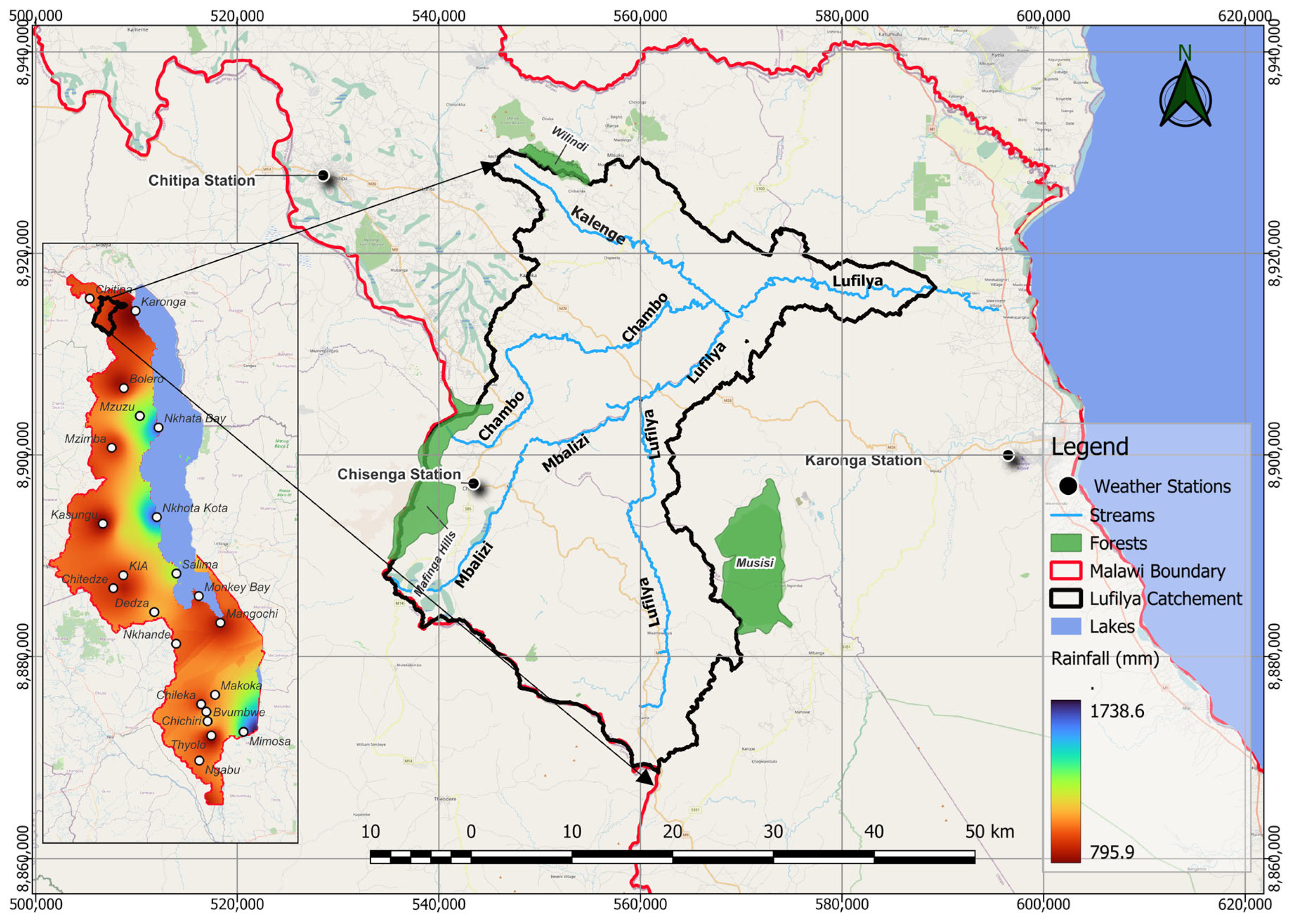[14] used SPI to evaluate maize vulnerability to drought in southern Malawi, their study did not include future climate change impacts. Thus, this study aims to project the future occurrence of meteorological droughts using the SPI indicator and future climate projections for the Lufilya River catchment. This catchment was selected because it supplies one of the largest and oldest irrigation schemes in Karonga, which has been severely affected by droughts and floods. Specifically, this study will (i) evaluate future climate change patterns for two periods (2025–2069 and 2070–2100) and (ii) calculate 3-month SPIs for both periods.

2. Materials and Methods

2.1. Study Area

The Lufilya catchment is located in the northern part of Malawi, between 09.67° S and 033.81° E and 10.24° S and 033.31° E. Approximately 85% of the catchment lies in Chitipa District, with the remaining portion in Karonga District. The catchment is drained by the Lufilya River, which has five major tributaries. The Lufilya River is essential for irrigation in Karonga District, as it supplies the Lufilya Irrigation Scheme, an area of 400 hectares. This scheme is located in a zone categorized as a flood and drought hotspot by JICA [24].

The Lufilya catchment experiences a typical Malawian climate, with three distinct seasons: a hot-wet season, a cool-dry season, and a hot-dry season [26]. On average, this catchment receives about 1000 mm of rainfall during the rainy season from November to April, with temperatures ranging from 22 °C to 24 °C. During the cool-dry season, between May and July, temperatures range from 18 °C to 20 °C, and in the hot-dry season, between August and October, temperatures range from 19 °C to 24 °C [27].

Land use in the Lufilya catchment is predominantly agricultural, with both crop and livestock farming. Other areas are covered by forest reserves, including Mafinga Hills in the southwestern part, Wilindi Forest Reserve in the northern part, and Musisi Forest Reserve in the southeastern part. A small portion of the catchment is built-up and includes bare land. The catchment features predominantly sandy loam and sand clay soils, with a smaller area covered by loamy sand soils.

2.2. Data Source and Description

2.2.1. Climatic Data

This study used rainfall and temperature data (both minimum and maximum) from the Chitipa, Karonga, and Chisenga weather stations, as there are not enough weather stations in the Lufilya catchment to accurately represent its climatic patterns (Figure 1). All data were obtained from the Meteorological Services of Malawi. A description of the data is shown in

Table 1. Climatic data description summary.

Data	Year Span	Missing Percentage	Time Scale	Data Format
Rainfall	1976–2015	0.0%	Monthly	Spread Sheet
Minimum Temperature	1976–2015	8.60%	Daily	Spread Sheet
Maximum Temperature	1976–2015	8.0%	Daily	Spread Sheet

. In this study, missing data were filled using the seasonal average method. Additionally, the data were tested for normality using the Shapiro–Wilk test [28], and outliers were identified using Dixon’s test.

2.2.2. Climate Change Projections Data

In this study, three Regional Climate Models (RCMs) from the Coordinated Regional Climate Downscaling Experiment (CORDEX) Africa were used to project future climate change scenarios. To reduce uncertainties associated with using a single RCM, an ensemble of three RCMs was selected [29,30]. The selection criteria focused on how well these models captured the seasonal patterns typical of the Malawian climate. All three RCMs fall within the AFR-44 or AFR-22 domains. The specific models used were CCLM4-8-17, REMO2009, and RCA4, coupled with two Representative Concentration Pathway (RCP) scenarios: the high-emission scenario (RCP8.5) and the intermediate-emission mitigation scenario (RCP4.5).

To project the degree of future climate change, the period from 1976 to 2005 was chosen as the historical baseline, with two future periods considered: 2025 to 2069 and 2070 to 2100. The data, available in NetCDF format with a resolution of 0.44° × 0.44° (approximately 50 km by 50 km), were extracted for the Chitipa weather station using the Python library NetCDF4 [31]. Although CMIP6 Global models are the successors to CMIP5 and have been deemed more reliable by researchers [32,33], this study used RCMs because they provide a finer-scale representation of climate in Eastern Africa [5] and in mountainous areas [34].

2.3. Bias Correction of Climate Change Data

Regional Climate Models (RCMs) are not typically used directly due to the potential introduction of biases, primarily caused by systematic model errors and the spatial resolution of data pixel cells [35]. As a result, it is necessary to apply bias correction to these data. Typically, remotely sensed data are bias-corrected using techniques such as linear scaling or probability distribution mapping [35,36]. In this study, the Quantile Mapping (QM) technique was employed to bias-correct both precipitation and temperature outputs from the RCMs. QM was chosen because it is widely used and has shown superior performance in similar studies conducted in Africa, including those by Dibaba et al. [29], Maharjan et al. [37], Teutschbein and Seibert [35], and Valdés-Pineda et al. [38].

Quantile Mapping (QM) adjusts the simulated data by aligning its probability distribution with that of observed data [18,38]. For this process, the Gamma Probability Distribution Function (GPDF) was used as the transfer function, as it has been shown in multiple studies to accurately model rainfall distributions [36,38]. The following is the GPDF transfer model:

$$\mathrm{G}\mathrm{P}\mathrm{D}\mathrm{F}\left(y_{yr,i,j,k}\right)={\displaystyle \frac{\mathrm{e}\mathrm{x}\mathrm{p}(-\frac{y_{yr,i,j}}{\mathrm{\varnothing }})x_{yr,i,j,k}^{\left(\Delta -1\right)}}{\Gamma \left(\Delta \right){\mathrm{\varnothing }}^{\Delta }}}$$

(1)

where $y_{yr,i,j,k}$ represents the time series of monthly rainfall data for year ($yr$) at location $i,j$ for RCM model $k$; $\Delta$ denotes the distribution shape parameter and $\varnothing$ represents the distribution scale parameter; and $\Gamma \left(\Delta \right)$ is the GPDF evaluated at $\Delta$. The GPDF parameters were calculated using product moments (PM) with the U.S. Army Corps of Engineers Hydrologic Engineering Center’s (HEC) Statistical Software Package (HEC-SSP). The gamma cumulative distribution function was used to calculate the probability of each $y_{yr,i,j,k}$ for simulated values. These simulated probabilities were then transformed using the inverse gamma distribution function with the observed GPDF parameters, as shown in Equation (2) below:

$${\left(y_{yr,i,j,k}\right)}_{correct}={GPDF}^{-1}(P_{\left(yr,i,j\right)},{\Delta }_{obs},{\mathrm{\varnothing }}_{obs})$$

(2)

where ${\left(y_{yr,i,j,k}\right)}_{correct}$ represents the corrected RCM time series of monthly rainfall data for year yr at location $i,j$ and the RCM model $k$, and ${\Delta }_{obs}$ and ${\mathrm{\varnothing }}_{obs}$ are the observed GPDF shape and scale parameters, respectively. If the percent bias between the observed and simulated rainfall is satisfactory, i.e., less than 20%, then the observed shape and scale GPDF parameters were used to bias-correct future simulated rainfall under both RCP4.5 and RCP8.5, because Quantile Mapping (QM) assumes that the statistical properties of the historical data remain unchanged when projecting future climatic variables [37].

A similar approach was applied to bias-correct temperature data, using distribution functions such as Log-Normal and Log-Pearson Type III. In this study, monthly data for the rainy season were analyzed separately from the dry season months to remove the seasonality effect from the data.

2.4. Drought Modelling Using Standard Precipitation Index (SPI)

The Standardized Precipitation Index (SPI) was calculated as a standard Z-score, following the method outlined by McKee et al. [39]. Typically, SPI is calculated by mapping rainfall values from one probability distribution to a normal distribution [10,40]. In this study, a 3-month moving average of monthly rainfall data was fitted to a Gamma distribution function. A 3-month period was chosen because it is the finest temporal resolution among the recommended periods for short-term drought analysis [14,41], as any period shorter than that might not represent drought adequately. The cumulative Gamma distribution was then transformed into a normal distribution with a mean of 0 and a standard deviation of 1 to determine the Z-score for each 3-month average. This approach was adopted from McKee et al. [39] and Şen [10].

This procedure was applied to both historical and projected rainfall data under two RCP scenarios (4.5 and 8.5) for the time windows 2025–2069 and 2070–2100. Drought occurrences were then categorized based on the classification system outlined by Al-Faraj et al. [42] and Khoi et al. [38] in

Table 2. SPI drought classification criteria.

SPI Value	Drought Classification
≥2.0	Extremely wet
1.5 to 1.99	Severely wet
1.0 to 1.49	Moderately wet
−0.99 to 0.99	Near normal
−1.0 to −1.49	Moderately dry
−1.5 to −1.99	Severely dry
≤−2.0	Extremely dry

.

3. Results

3.1. Bias Correction

All rainfall data fit well to a Gamma distribution shown in Figure 2, Figure 3, Figure 4 and Figure 5. After applying Quantile Mapping (QM) to the historically simulated rainfall data across all RCMs, the percentage bias (PBIAS) was significantly reduced. Most of the historically simulated temperature data showed small biases, except for RCA4, where the minimum temperature had a substantial bias of −11%. These data were then corrected using QM, with the Log-Normal probability distribution proving to be a good fit for both observed and simulated minimum temperature data. As a result, the Log-Normal distribution was selected for QM, reducing the bias from −11% to −0.042%.

Table 3. Bias of RCM models before and after application of QM for Chisenga weather station.

RCM Model	Months
	January		February		March		April		November		December
	Bias Before QM	Bias After QM	Bias Before QM	Bias After QM	Bias Before QM	Bias After QM	Bias Before QM	Bias After QM	Bias Before QM	Bias After QM	Bias Before QM	Bias After QM
CCLM4-8-17	19.98%	−0.03%	17.59%	0.02%	−10.14%	0.05%	−60.14%	−3.49%	167.12%	−0.22%	141.41%	0.19%
REMO2009	−27.54%	−0.01%	−46.57%	0.10%	−58.38%	−0.15%	−78.44%	−5.09%	128.04%	−1.74%	24.60%	−0.08%
RCA4	199.23%	−0.03%	204.16%	−0.06%	77.18%	−0.02%	−37.63%	0.10%	502.10%	0.68%	519.90%	0.03%

,

Table 4. Bias of RCM models before and after application of QM for Chitipa weather station.

RCM Model	Months
	January		February		March		April		November		December
	Bias Before QM	Bias After QM	Bias Before QM	Bias After QM	Bias Before QM	Bias After QM	Bias Before QM	Bias After QM	Bias Before QM	Bias After QM	Bias Before QM	Bias After QM
CCLM4-8-17	1.00%	1.00%	−8.59%	−0.17%	−16.83%	−3.16%	−50.92%	−10.60%	−0.39%	−0.39%	5.26%	5.26%
REMO2009	−19.75%	2.35%	−19.23%	−0.14%	−18.32%	−3.11%	−27.80%	−4.08%	89.57%	−3.23%	3.99%	3.99%
RCA4	−37.65%	2.27%	−36.34%	−0.16%	−40.41%	−3.32%	−60.84%	−4.41%	−15.52%	−4.01%	−19.20%	−5.57%

and

Table 5. Bias of RCM models before and after application of QM for Karonga weather station.

RCM Model	Months
	January		February		March		April		November		December
	Bias Before QM	Bias After QM	Bias Before QM	Bias After QM	Bias Before QM	Bias After QM	Bias Before QM	Bias After QM	Bias Before QM	Bias After QM	Bias Before QM	Bias After QM
CCLM4-8-17	1.67%	0.06%	1.05%	−0.02%	−36.31%	−0.05%	−60.71%	−3.36%	30.75%	−1.25%	3.16%	−0.10%
REMO2009	35.59%	0.00%	5.04%	−0.02%	−39.49%	−0.54%	−36.95%	0.02%	129.47%	−0.72%	30.62%	−0.12%
RCA4	−96.45%	−0.56%	−95.29%	0.98%	−96.75%	0.85%	−97.43%	−6.45%	−94.93%	20.92%	−95.56%	2.02%

below provide a summary of how QM effectively reduced the bias in the simulated data.

3.2. Future Climate Change Projections

Bias-corrected future climatic precipitation and temperature data were used to illustrate the projected increases or decreases in these variables relative to the baseline climatic period (1976–2005). Both the outputs of individual RCMs and the ensemble means were compared against the baseline temperature and precipitation data.

3.2.1. Precipitation

Annual Variation in Projected Precipitation

The average precipitation for both individual RCMs and the ensemble projections was analyzed for future precipitation under RCP4.5 and RCP8.5, across the time periods 2025–2069 and 2070–2100, and compared against baseline precipitation averages. The results indicate that all RCMs, across both time periods and emission scenarios, project an increase in rainfall.

Among all the RCMs, REMO2009 consistently projected a smaller increase in rainfall for the near-future window (2025–2069) across all RCPs. For instance, REMO2009 projected a 67% increase compared to an 85% increase for RCA4 and 74.4% for CCLM4-8-17. Despite RCA4 projecting the greatest increase in rainfall (85%) for the near-future period (2025–2069) across all RCPs, it projected the smallest increase in rainfall (40%) for the far-future period.

According to

Table 6. Percentage change of precipitation for RCMs and ensemble precipitation projection.

RCMs	RCP 4.5		RCP 8.5
	2025–2069	2070–2100	2025–2069	2070–2100
CCLM4-8-17	74.4%	63.8%	72.5%	68.4%
REMO2009	67.3%	76.8%	66.6%	76.9%
RCA4	85.0%	40.1%	84.9%	40.1%
Ensemble	75.6%	60.2%	74.7%	61.4%

, the ensemble means suggest that for the far future, RCP8.5 projects more rainfall than RCP4.5, while RCP4.5 projects more rainfall for the near-future period than RCP8.5. A summary of the percentage change in precipitation for each RCM and ensemble projection is provided in Table 6 below.

Monthly Variations in Projected Precipitation

On a monthly scale, the results indicate that the RCMs generally project an increase in rainfall for wetter months and a decrease for drier months. For example, Figure 6, Figure 7, Figure 8, Figure 9, Figure 10 and Figure 11 show that during the onset of the rainy season (November and December), none of the RCMs projected an increase in precipitation. In contrast, all RCMs projected an increase in rainfall from January to April. Furthermore, Figure 6, Figure 7, Figure 8, Figure 9, Figure 10 and Figure 11 illustrate that for CCLM4-8-17 under RCP4.5 radiation forcing, monthly rainfall was projected to be higher compared to RCP8.5 radiation forcing. On the other hand, the opposite was true for RCA4 and REMO2009.

3.2.2. Temperature

Annual Variations in Projected Temperature

Bias-corrected projected maximum and minimum temperatures under both RCP4.5 and RCP8.5 for future periods indicate that the diurnal temperature range will increase across all RCMs. For instance, all RCMs under both RCPs project a decrease in minimum temperature across all future periods, with RCP4.5 showing a greater reduction in minimum temperature than RCP8.5 for the same periods. Conversely, all RCMs under both RCPs forecast an increase in maximum temperature across all future periods, with a more significant rise noted under RCP8.5 compared to RCP4.5. However, CCLM4-8-17 projected a slight decrease in maximum temperature in the near future (2025–2069) of −2.4% and in the far future (2070–2100) of −0.08%.

The results also indicate that, in most cases, all RCMs project higher temperatures for the far-future period compared to the near-future period, except for CCLM4-8-17 under RCP4.5. The REMO2009 RCM projected the highest minimum and maximum temperatures across all RCPs and future periods, except for RCP8.5 in the near-future period (2025–2069), during which RCA4 consistently exhibited higher minimum and maximum temperatures than all other models. All RCMs under all emission scenarios projected an increase in daily average temperatures, with the exception of CCLM4-8-17, which forecasted a slight decrease in temperature, excluding the far-future period under RCP8.5.

Ensemble averages indicate that temperatures are expected to rise by 1% between 2025–2069 and 6.5% between 2070 and 2100 under RCP4.5. The average temperature is projected to increase by 3.7% between 2025 and 2069 and 12.7% between 2070 and 2100. A summary of the percentage changes in minimum, maximum, and average temperatures is presented in

Table 7. Percentage change of minimum temperature for RCMs and all future periods.

RCMs	RCP 4.5 Minimum Temperature Change		RCP 8.5 Minimum Temperature Change
	2025–2069	2070–2100	2025–2069	2070–2100
CCLM4-8-17	−23.90%	−25.00%	−26.70%	−21.63%
REMO2009	−25.28%	−22.38%	−23.06%	−14.14%
RCA4	−23.90%	−18.91%	−21.93%	−10.03%
Ensemble	−24.36%	−22.10%	−23.90%	−15.27%

,

Table 8. Percentage change of maximum temperature for RCMs and all future periods.

RCMs	RCP 4.5 Maximum Temperature Change		RCP 8.5 Maximum Temperature Change
	2025–2069	2070–2100	2025–2069	2070–2100
CCLM4-8-17	−2.40%	−0.08%	0.04%	9.42%
REMO2009	4.82%	8.25%	1.23%	15.34%
RCA4	2.73%	7.36%	4.03%	14.68%
Ensemble	1.72%	8.64%	2%	13.1%

and

Table 9. Percentage change of average temperature for All RCMs and all future periods.

RCMs	RCP 4.5 Average Temperature Change		RCP 8.5 Average Temperature Change
	2025–2069	2070–2100	2025–2069	2070–2100
CCLM4-8-17	−1.37%	−0.48%	−1.25%	7.12%
REMO2009	2.54%	6.12%	1.41%	14.65%
RCA4	1.85%	7.22%	3.65%	16.20%
Ensemble	1.01%	6.49%	1.3%	12.7%

.

Monthly Variations in Projected Temperature

At the monthly scale, projected temperatures tend to increase more during the hotter months, specifically in the hot-wet and hot-dry seasons, compared to the cool-dry season. All RCMs consistently demonstrate this pattern, with the exception of REMO2009, which shows a contradictory trend. Across all RCMs and RCPs, temperatures are projected to rise more significantly toward the end of the century. This trend is clearly illustrated in Figure 12, Figure 13, Figure 14, Figure 15, Figure 16 and Figure 17.

3.3. Drought Prevalence

3.3.1. Historical Drought Prevalence

SPI values for historical rainfall indicate that moderate droughts occurred most frequently, followed by severe and extreme droughts, as shown in

Table 10. Decade-by-decade drought prevalence between 1976 and 2022.

Decades	Moderate Drought	Severe Drought	Extreme Drought	Frequency
1976–1985	4	2	0	6
1986–1995	5	6	4	15
1996–2005	5	4	3	12
2006–2015	9	1	1	12
2015–2022	4	1	1	6

. On a decade-by-decade basis, SPI analysis reveals that extreme and severe droughts were most frequent in the late 1990s and early 2000s, similar to the findings of Nangoma [43]. Longer negative spikes representing extreme droughts can be visualized in Figure 18, Figure 19 and Figure 20. Conversely, moderate droughts were more frequent in the mid-2000s, leading to shorter negative spikes, as observed in Figure 18, Figure 19 and Figure 20. These findings align with published data on the occurrence of major droughts in Malawi between 1992 and 2007 [24]. For instance, the SPI analysis indicated that extreme droughts occurred in 1987, 1990, 1992, 2003, and 2005. All these dates, except for 2003, appear in the historical results published by JICA [24].

3.3.2. Future Drought Prevalence

SPI analysis indicates that the frequency of extreme droughts under RCP 8.5 is increasing over time for both future periods. From

Table 11. Drought prevalence for near-future period (2025 to 2069).

Decades	Moderate		Severe		Extreme
	RCP 4.5	RCP 8.5	RCP 4.5	RCP 8.5	RCP 4.5	RCP 8.5
2025–2035	4	1	2	2	2	1
2036–2046	7	5	5	4	1	2
2047–2056	8	6	1	3	3	2
2057–2069	8	13	4	3	1	2
Total	27	25	12	12	7	7

and

Table 12. Drought prevalence in far-future period (2079 to 2100).

Decades	Moderate		Severe		Extreme
	RCP 4.5	RCP 8.5	RCP 4.5	RCP 8.5	RCP 4.5	RCP 8.5
2070–2079	6	9	3	0	0	0
2080–2089	12	13	6	3	0	2
2090–2100	6	10	6	3	0	3
Total	24	32	15	6	0	5

, RCP 4.5 projects no extreme droughts for the far-future period, and no clear pattern is shown for RCP 4.5 in the near-future, though, generally, the frequency of extreme droughts is increasing.

The results show that severe droughts increase over time under RCP 8.5 radiation forcing, whereas the ensemble RCM under RCP 4.5 projects no clear trend in severe droughts, though a higher frequency is projected in the 2040s and 2060s. From Table 10, results show that moderate droughts are projected to increase over time in the near-future period under both RCPs. However, Table 11 indicates that moderate droughts do not show a consistent increasing trend for either RCP. For both RCPs, the ensemble RCM projects that moderate droughts will be more common in the 2080s compared to projections for the 2070s and 2090s.

In comparison to historical drought prevalence, results show that the frequency of extreme droughts is projected to decrease by 51% under RCP 4.5 and by 15% under RCP 8.5 by 2100. In contrast, the frequency of moderate droughts is projected to increase by 25% under RCP 4.5 and by 39% under RCP 8.5 by the end of the century. The projection of severe droughts varies between RCPs, with RCP 4.5 projecting an increase of 14% in severe drought prevalence, while RCP 8.5 projects a 24% decrease in the frequency of severe droughts. This temporal variation in drought prevalence can be observed in Figure 21 and Figure 22 below.

The spatial distribution of drought frequency in

Table 13. Spatial distribution of drought frequency over the catchment.

	Moderate Droughts	Severe Droughts	Extreme Droughts
RCP 4.5 (2025–2069)
RCP 4.5 (2070–2100)
RCP 8.5 (2025–2069)
RCP 8.5 (2070–2100)

shows that extreme and moderate droughts are projected to increase in a northeastward direction across the catchment, while severe droughts show no general spatial pattern but are mostly projected to be more prevalent in the northern part of the catchment between 2025 and 2069 under both RCMs.

Generally, the results indicate that under RCP 8.5, a higher prevalence of droughts is projected for both time windows compared to RCP 4.5. For example, compared to historical drought prevalence, RCP 4.5 projects an 8% increase in drought prevalence, while RCP 8.5 projects an 11% increase in drought frequency.

4. Discussion

In this study, an ensemble of three downscaled Regional Climate Models (RCMs) projected an increase in rainfall across both RCP 4.5 and RCP 8.5 scenarios. Similar findings were reported by Vincent [22], who observed that most global circulation models projected an increase in wetting trends across northern and central Malawi. Adhikari and Nejadhashemi [23] also projected increased rainfall in northern Malawi, which includes the Lufilya catchment area. This consistency in results across studies highlights similar precipitation trends, even when conducted at coarser resolutions and with varying precipitation magnitudes. Other researchers have observed comparable patterns in other regions worldwide. For example, in India, Jasrotia et al. [44] found that under RCP 4.5, RCMs projected less rainfall than under RCP 8.5, although both RCPs forecast an increase in rainfall relative to baseline levels. Similarly, Gebre and Ludwig [19] projected an increase in rainfall across the Tana Basin in the upper Blue Nile region.

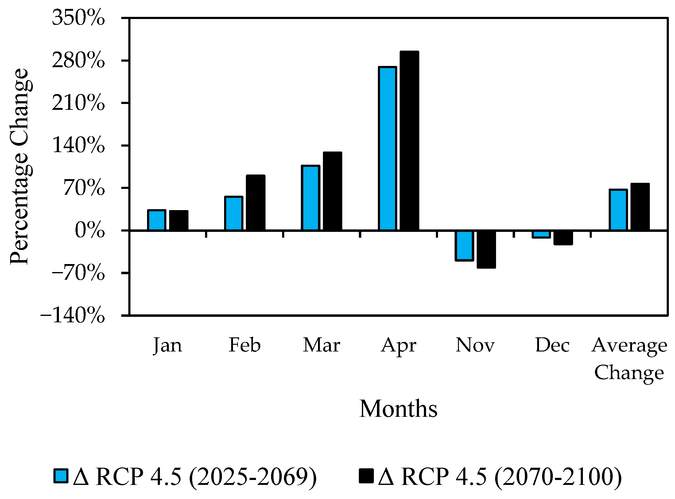
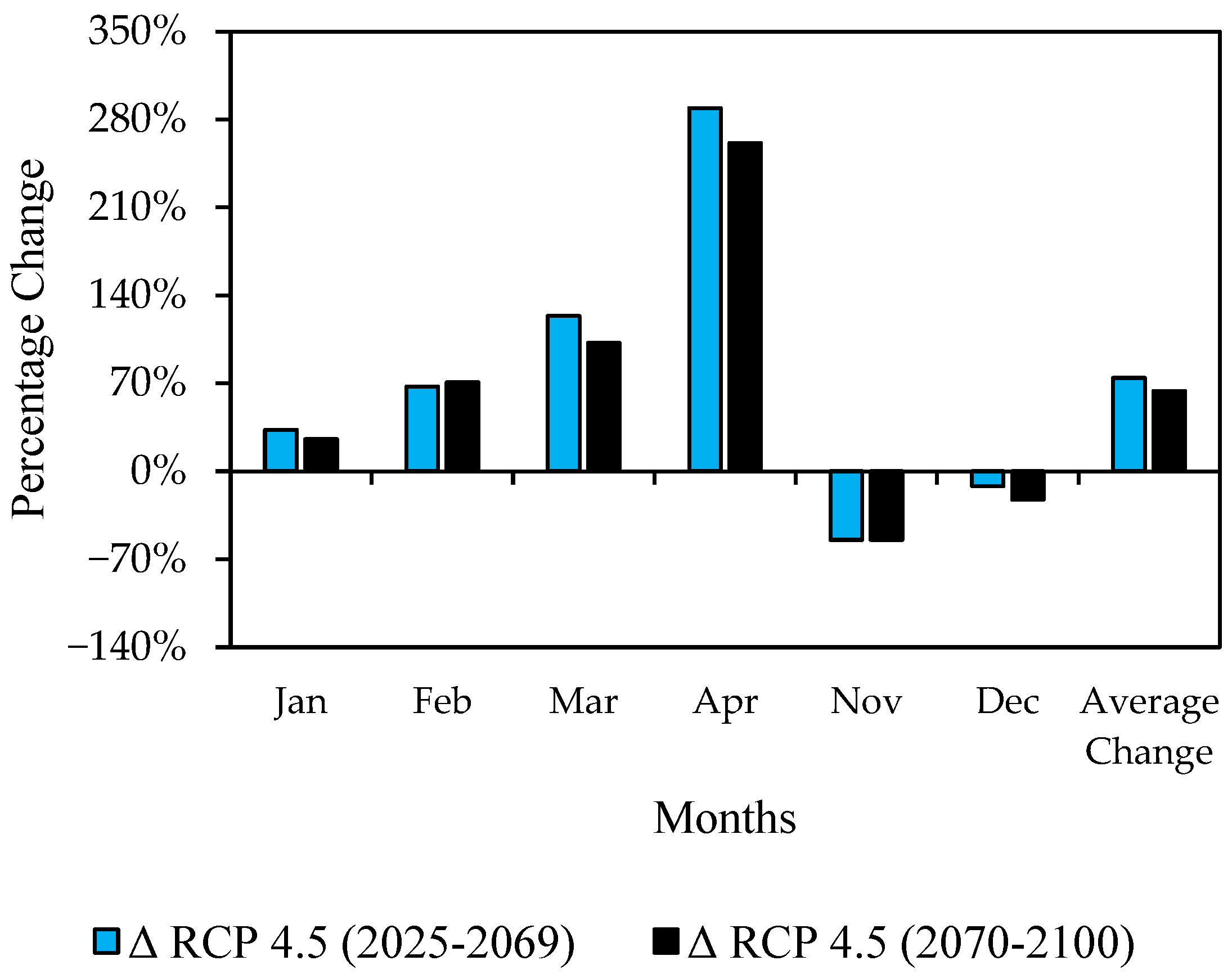
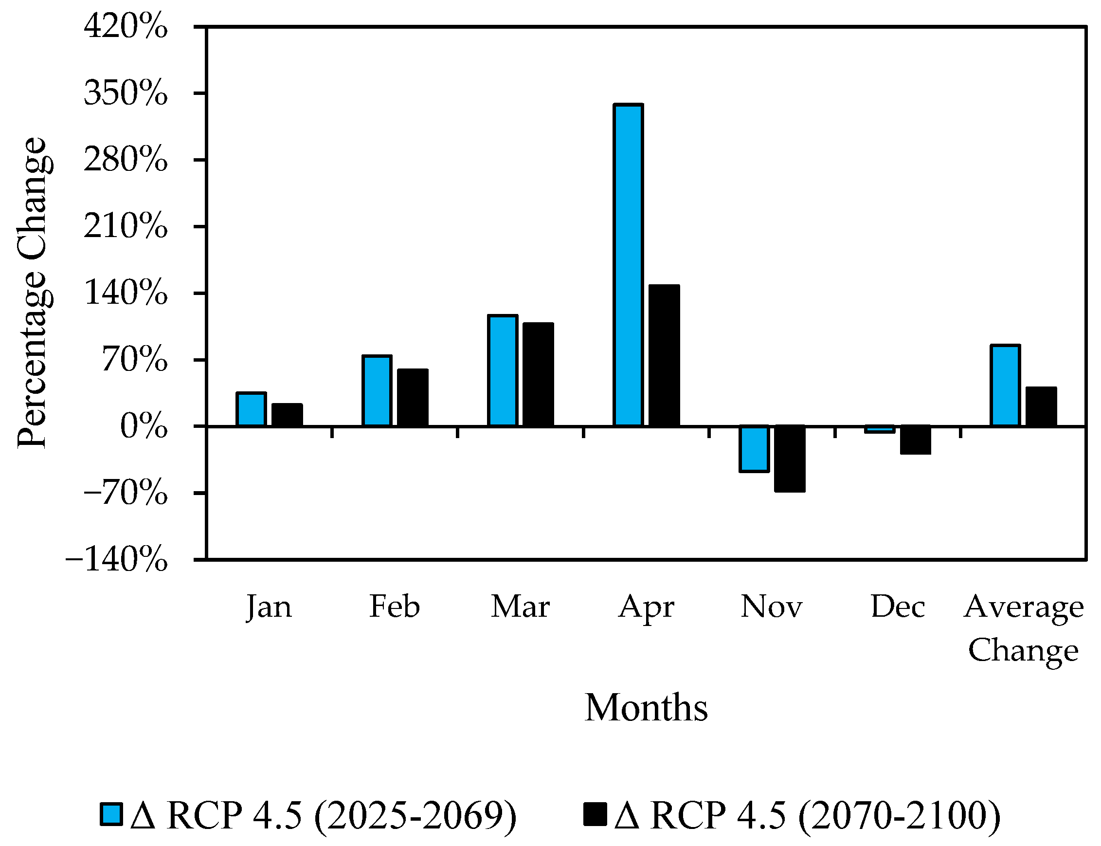
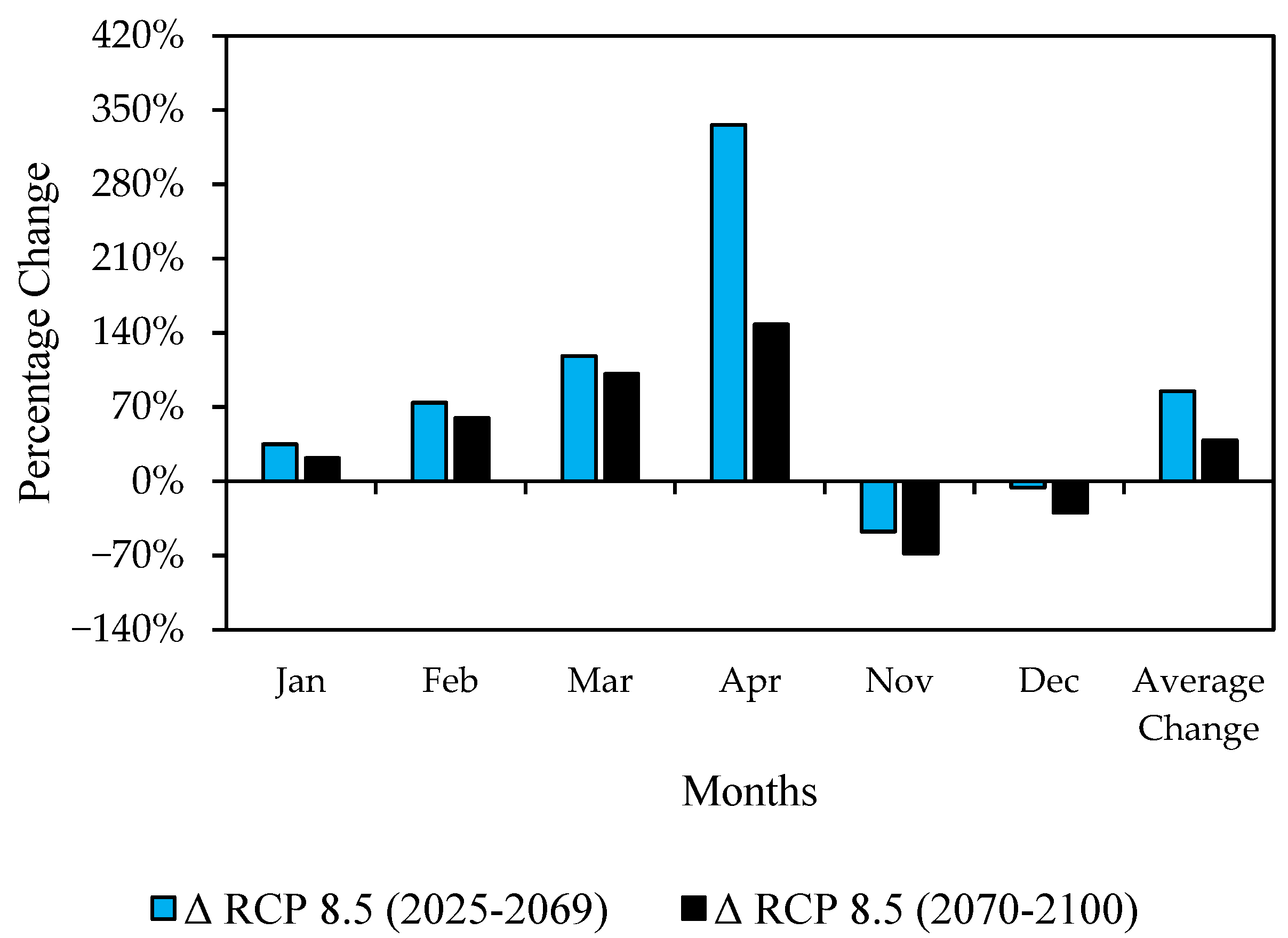
On a monthly basis, the analysis showed that rainfall is likely to increase during the wettest months and decrease during the drier months, specifically at the onset of the rainy season. Vincent [22] conducted a similar study in Malawi and reported a rainfall decrease of about 10% during the hot-dry season and an increase of about 4% during the wet season. This study, however, observed a greater range of variability, with rainfall increasing by 33% to 285% during the rainy season and decreasing by −59% to −11% at the onset and end of the rainy season. Haile et al. [45] in Ethiopia and Chattopadhyay et al. [46] in the United States also found comparable seasonal rainfall patterns in their studies. These variations may be attributed to increased evaporation and temperatures, which can lead to more humid conditions during wet months and drier conditions in dry months [47].

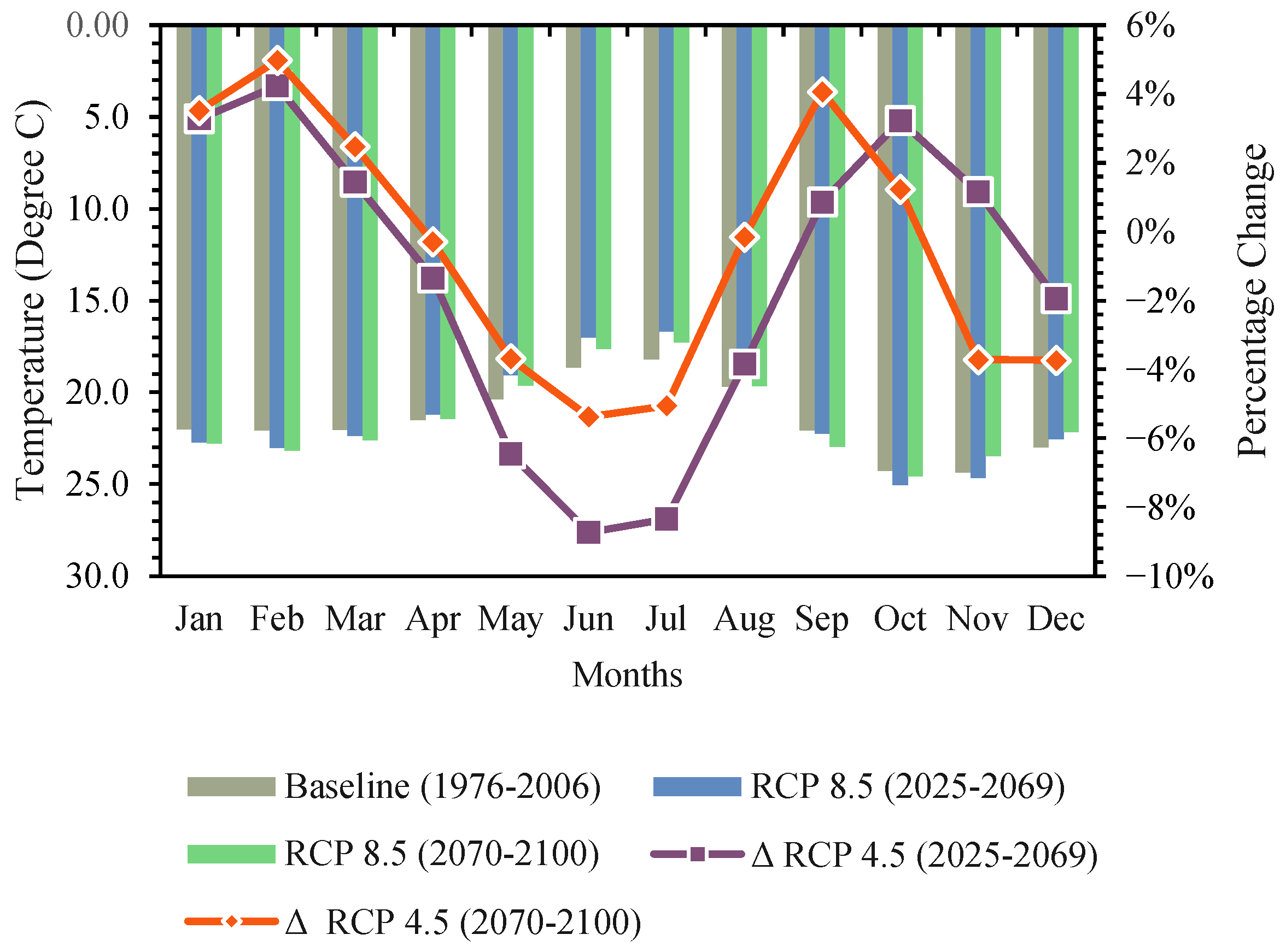
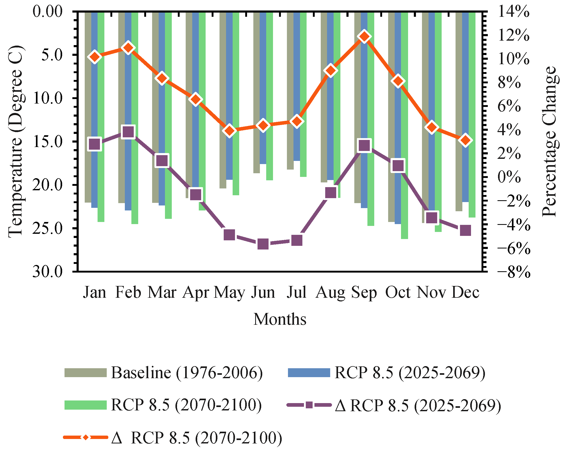
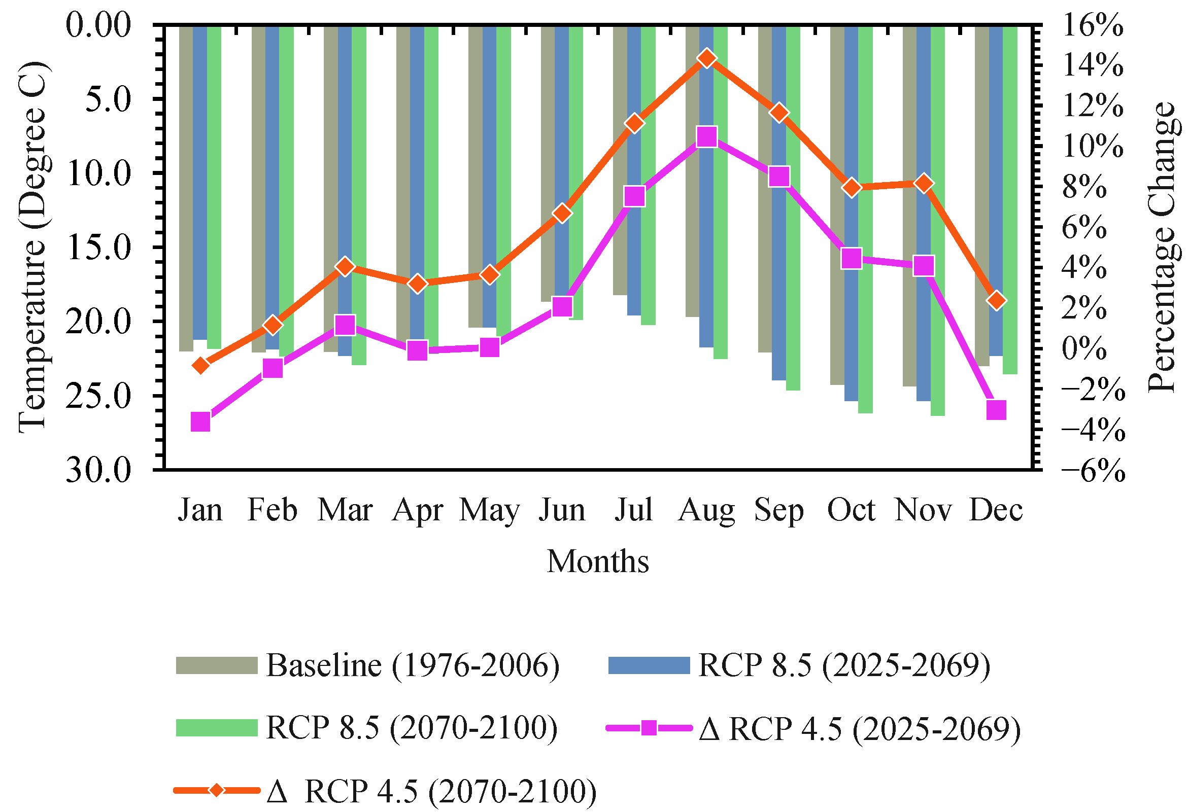
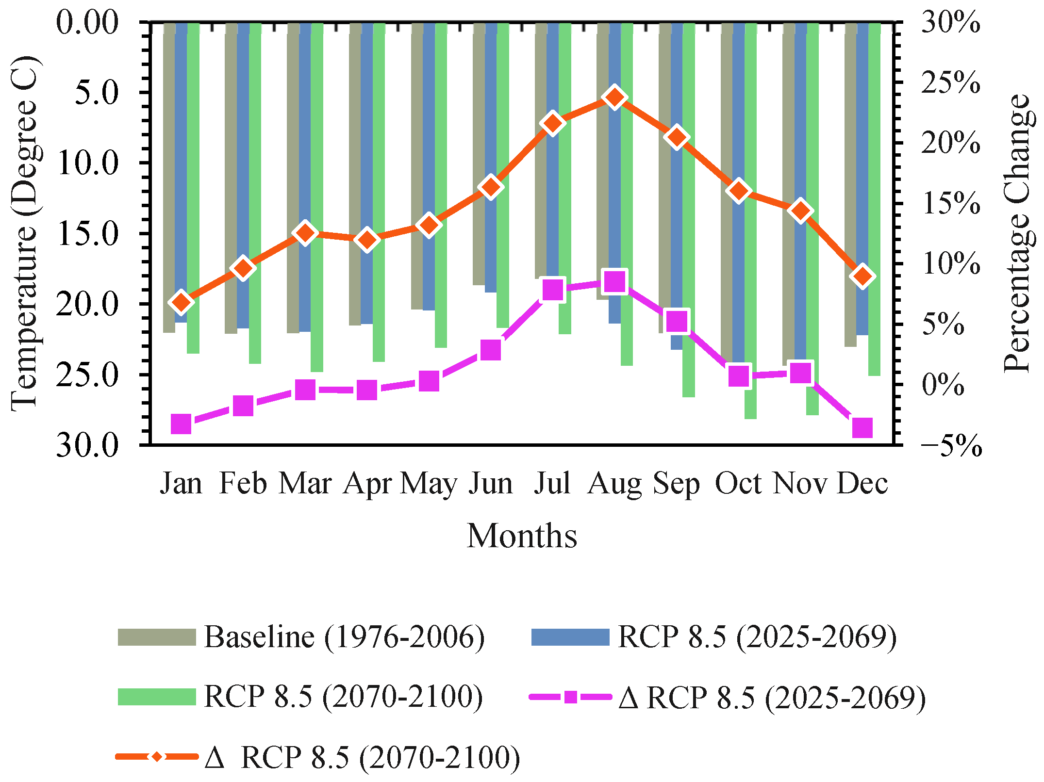
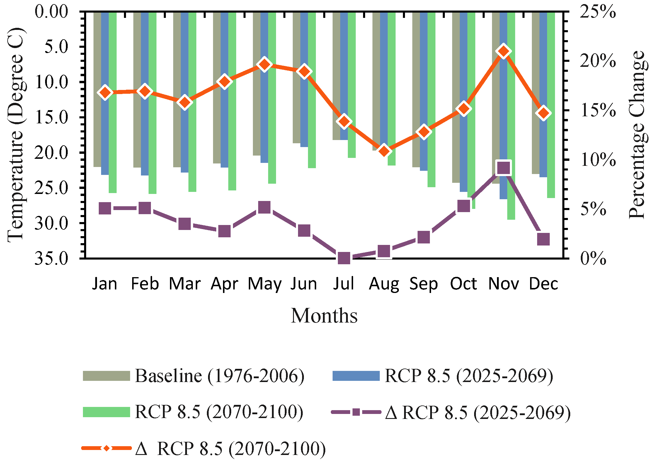
The ensemble average of the climate models also projects a general increase in average daily temperature. Similar increases in temperature across Malawi were projected by Vincent [22] and Adhikari and Nejadhashemi [23]. Comparable projections were also noted in other regions, such as Egypt (Elshamy et al. [48]), Ethiopia (Gadissa et al. [30] and Gebre and Ludwig [19]), Burma (Ghimire et al. [49]), and across Africa (Aich et al. [50]). Recently, Iyakaremye et al. [51] projected rapid increases in temperature extremes across southern Africa. Although all these studies indicated an increase in average annual temperatures, similar to this study, they also projected increases in both minimum and maximum temperatures, which contrasts with the results of this study. Vincent [22] observed that northern Malawi, particularly the highland and lakeshore areas, is expected to be colder, which could explain the projected decrease in minimum temperatures in this region.

From Figure 12, Figure 13, Figure 14 and Figure 15, it is evident that temperature is projected to increase more during colder months than in warmer months. Vincent [22] similarly found that the annual rate of temperature increase is lower in relatively colder months (March to May and December to February) compared to hotter months (September to November). Chattopadhyay et al. [46] observed a similar pattern in the Kentucky River Basin in the United States, where global circulation models (GCMs) projected a greater increase in temperature during summer than in spring.

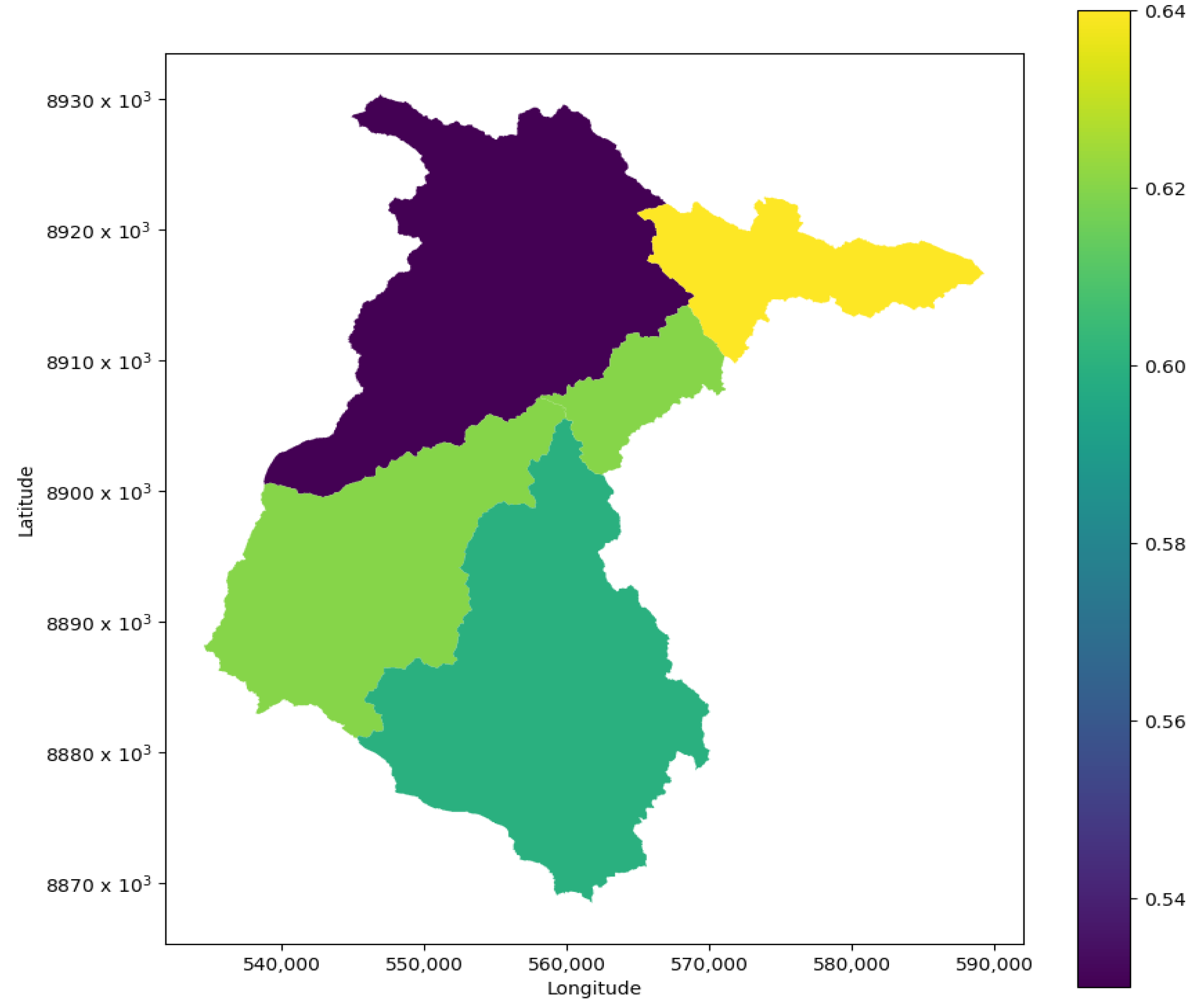
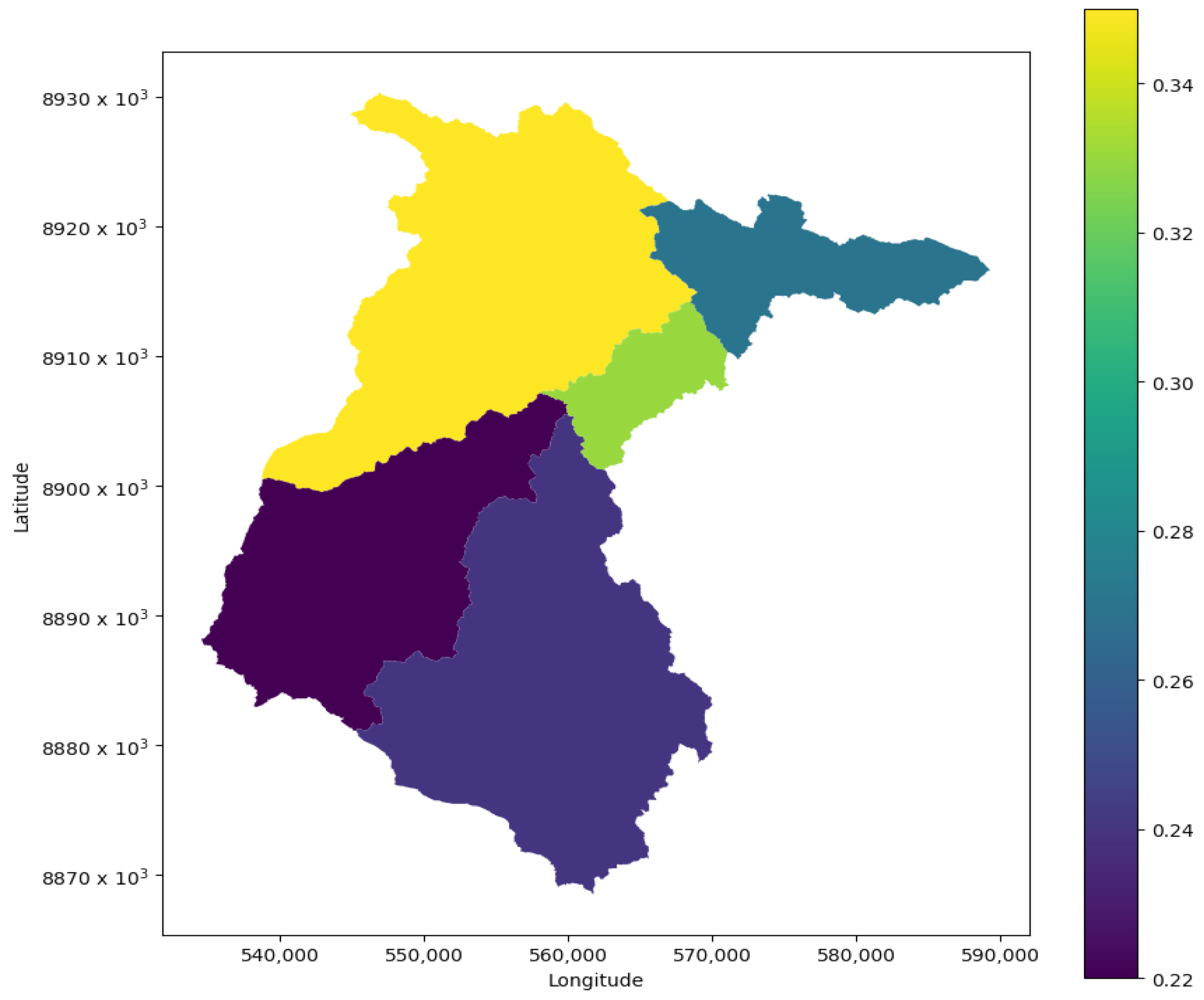
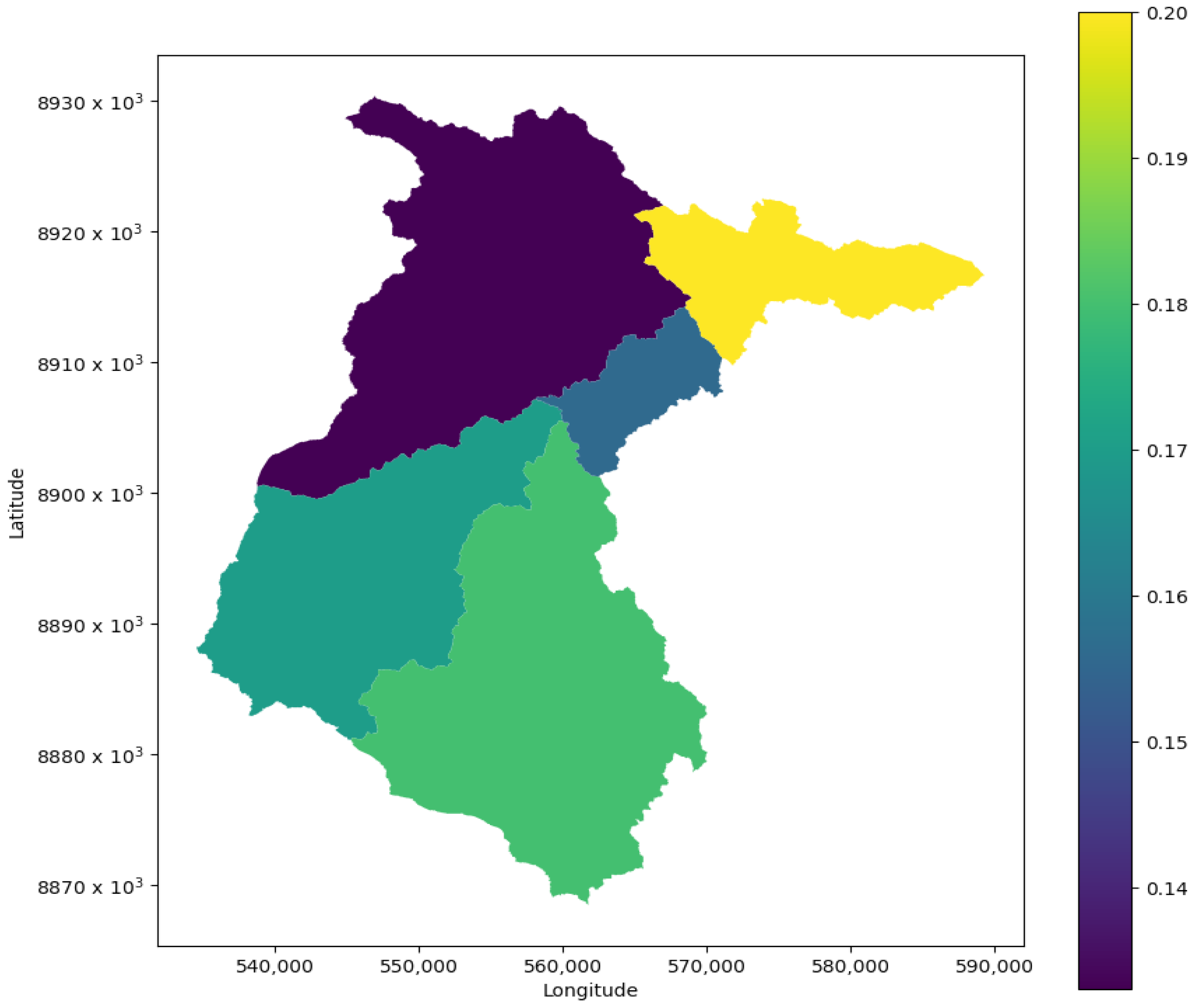
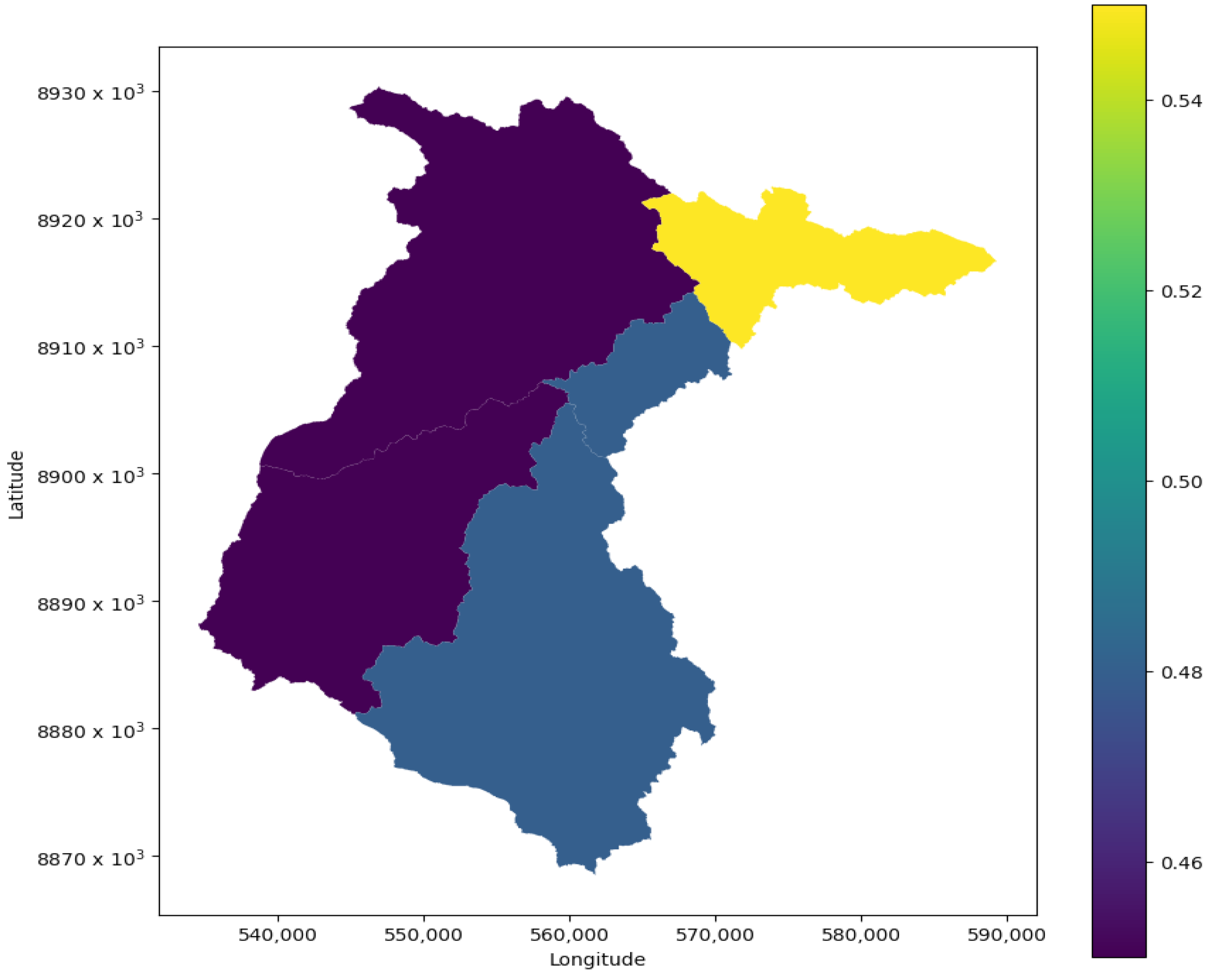
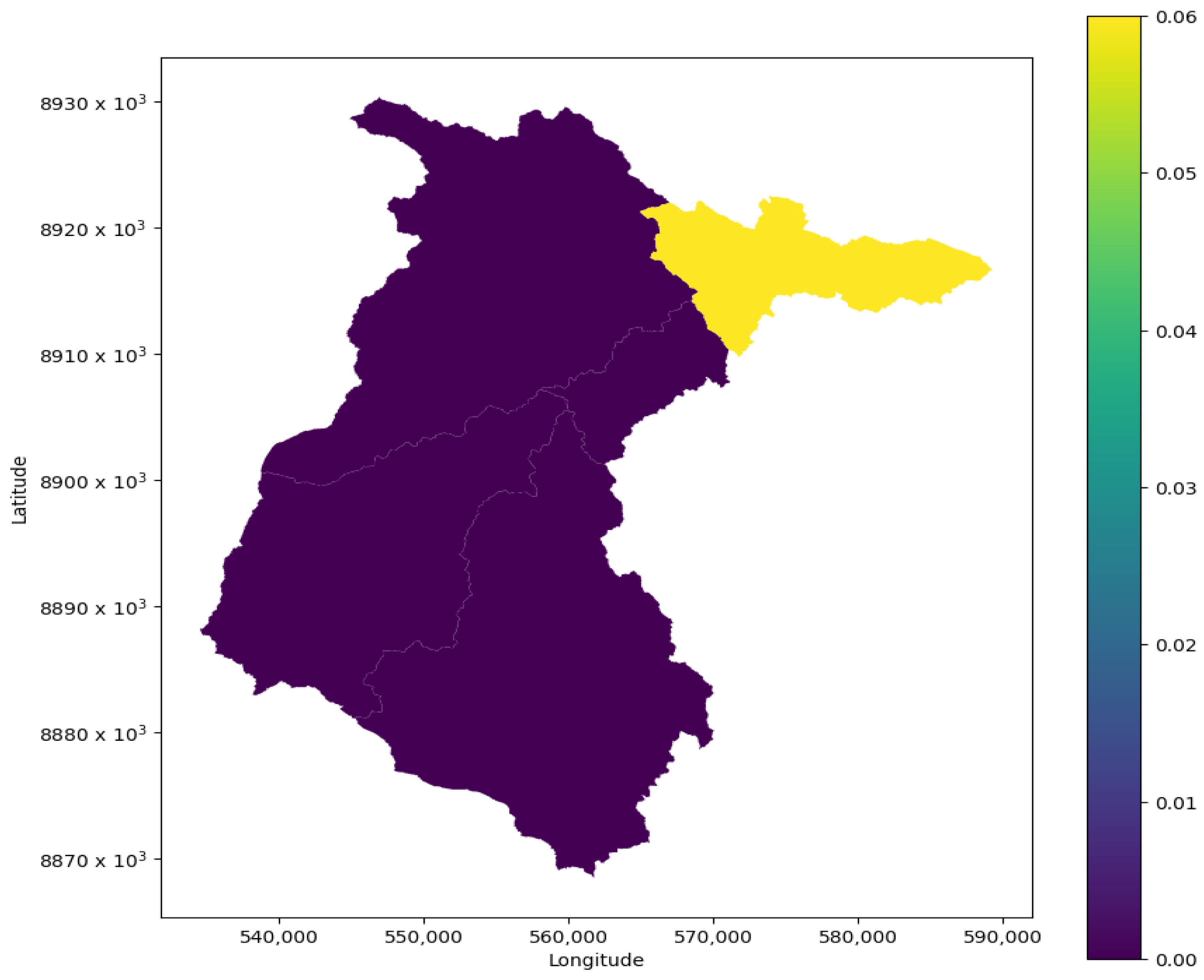
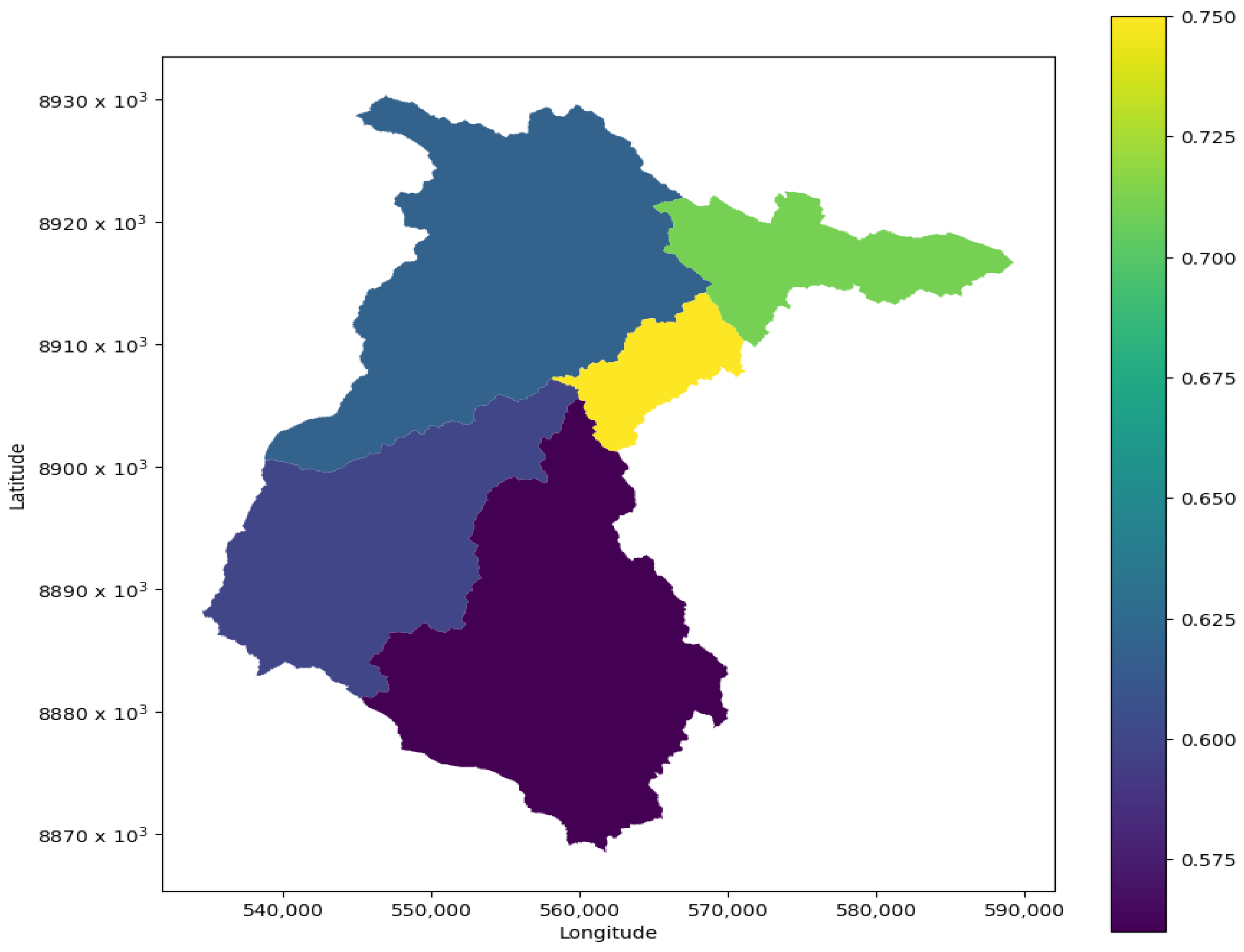
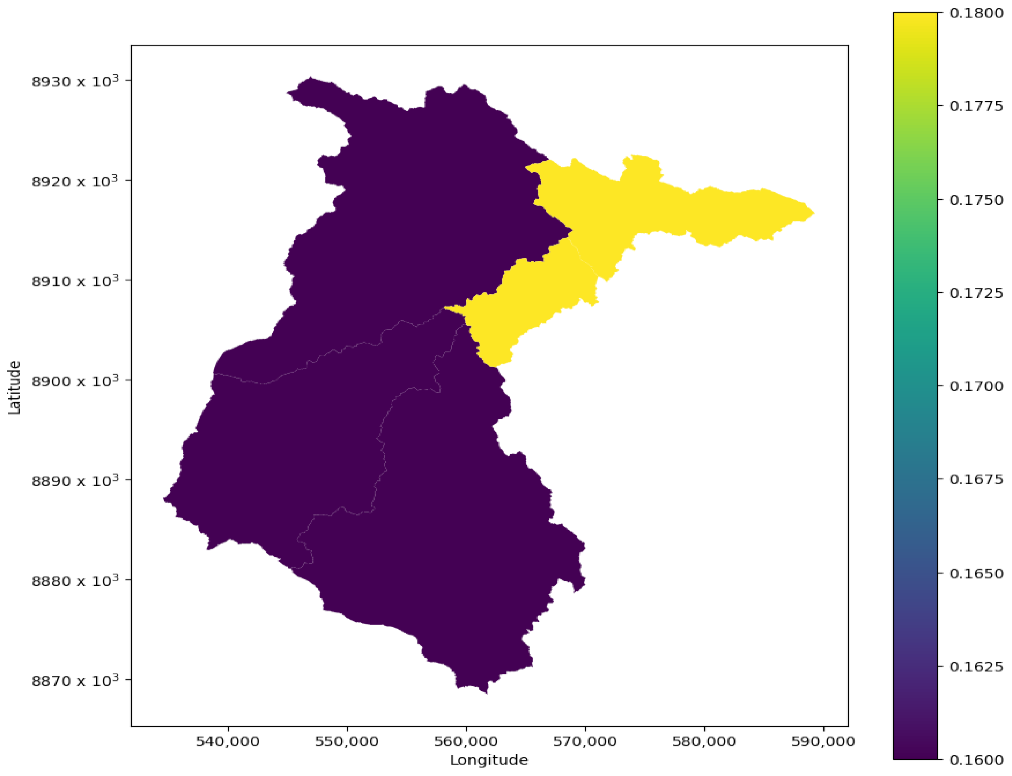
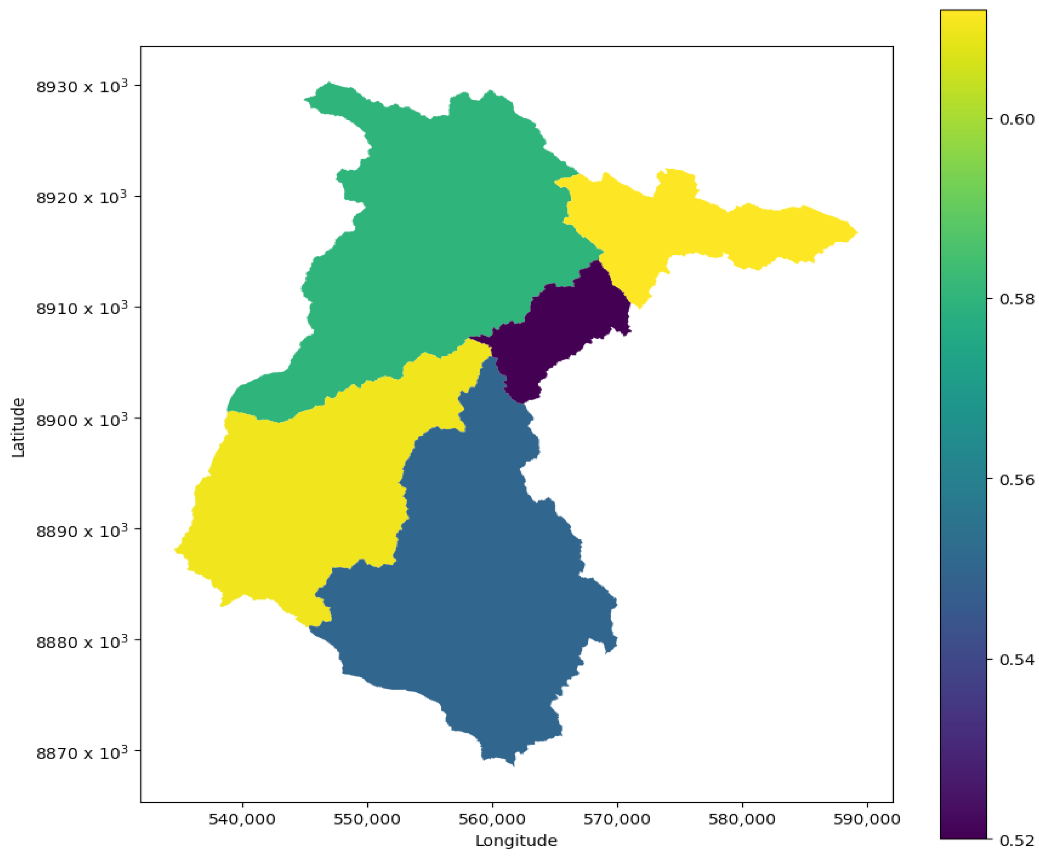
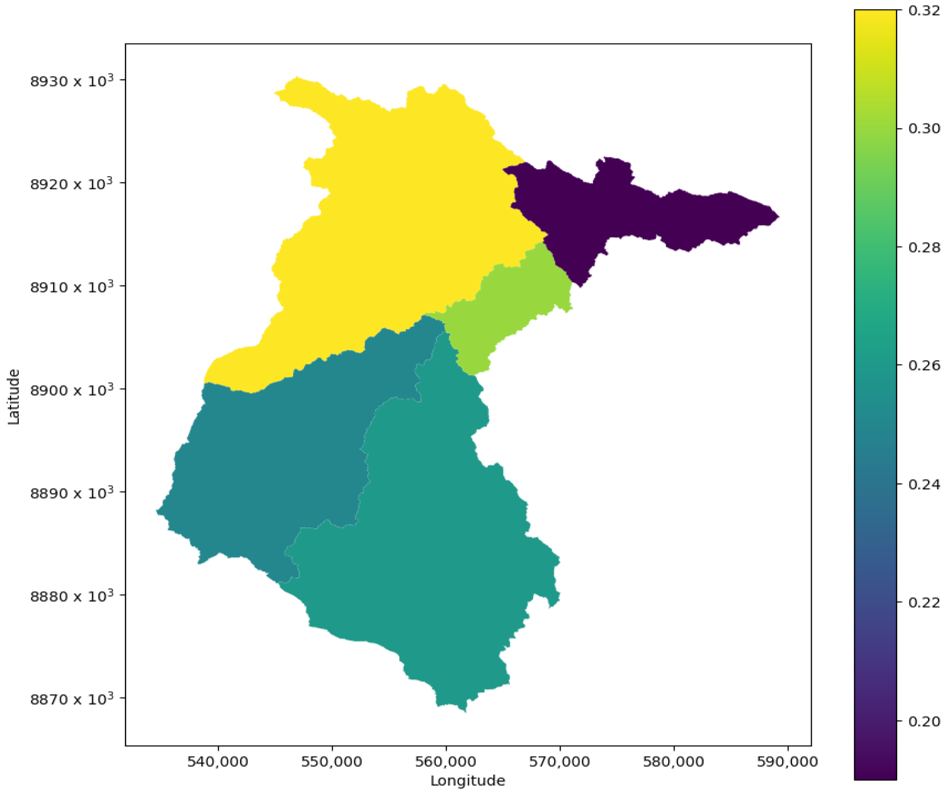
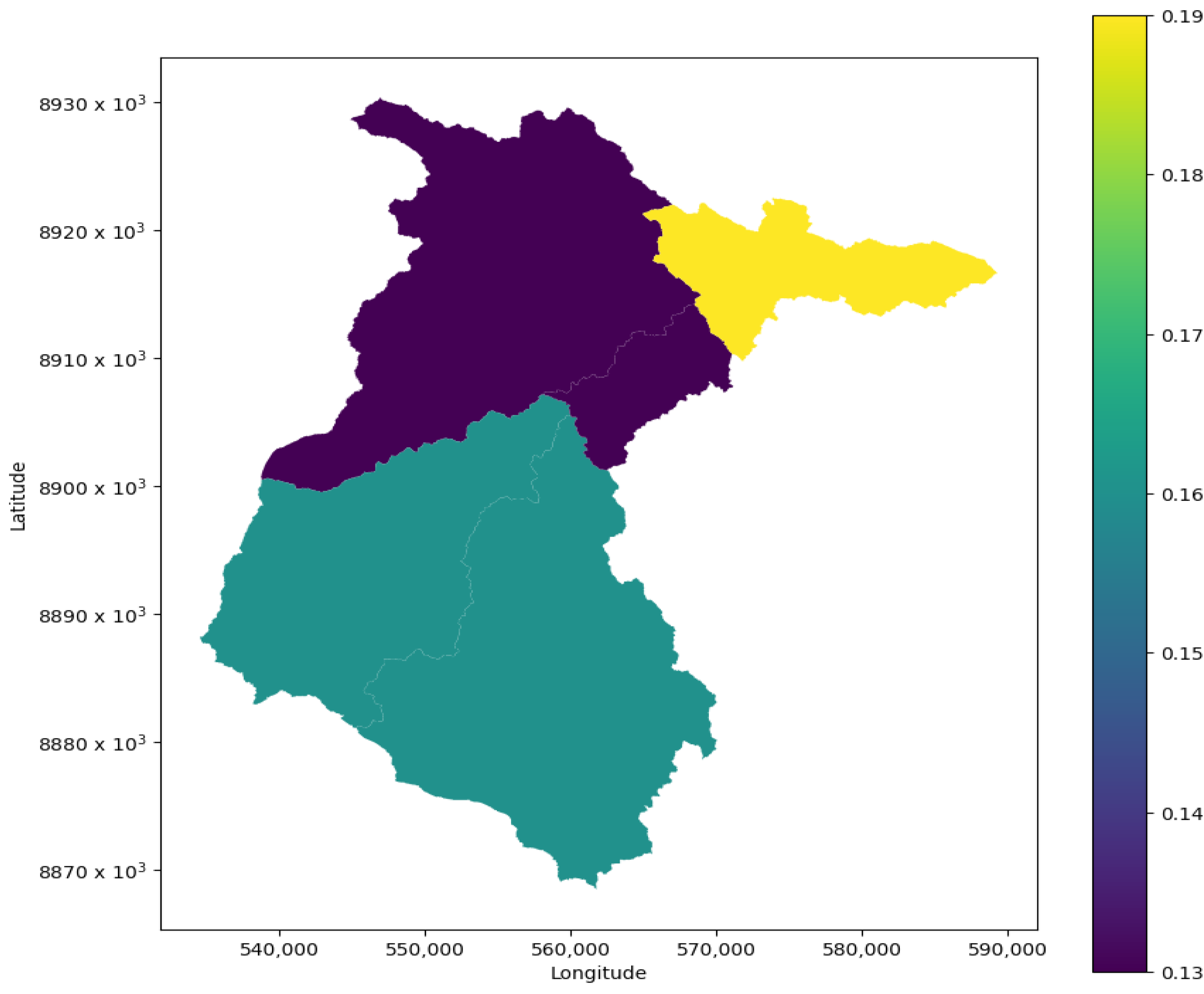
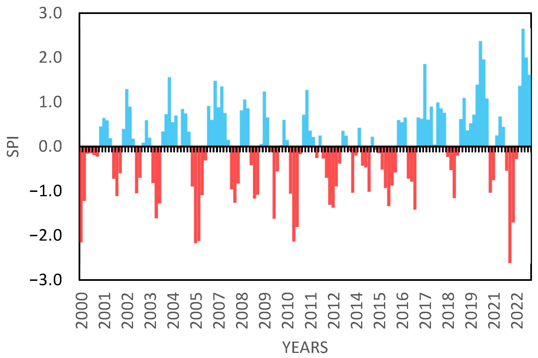
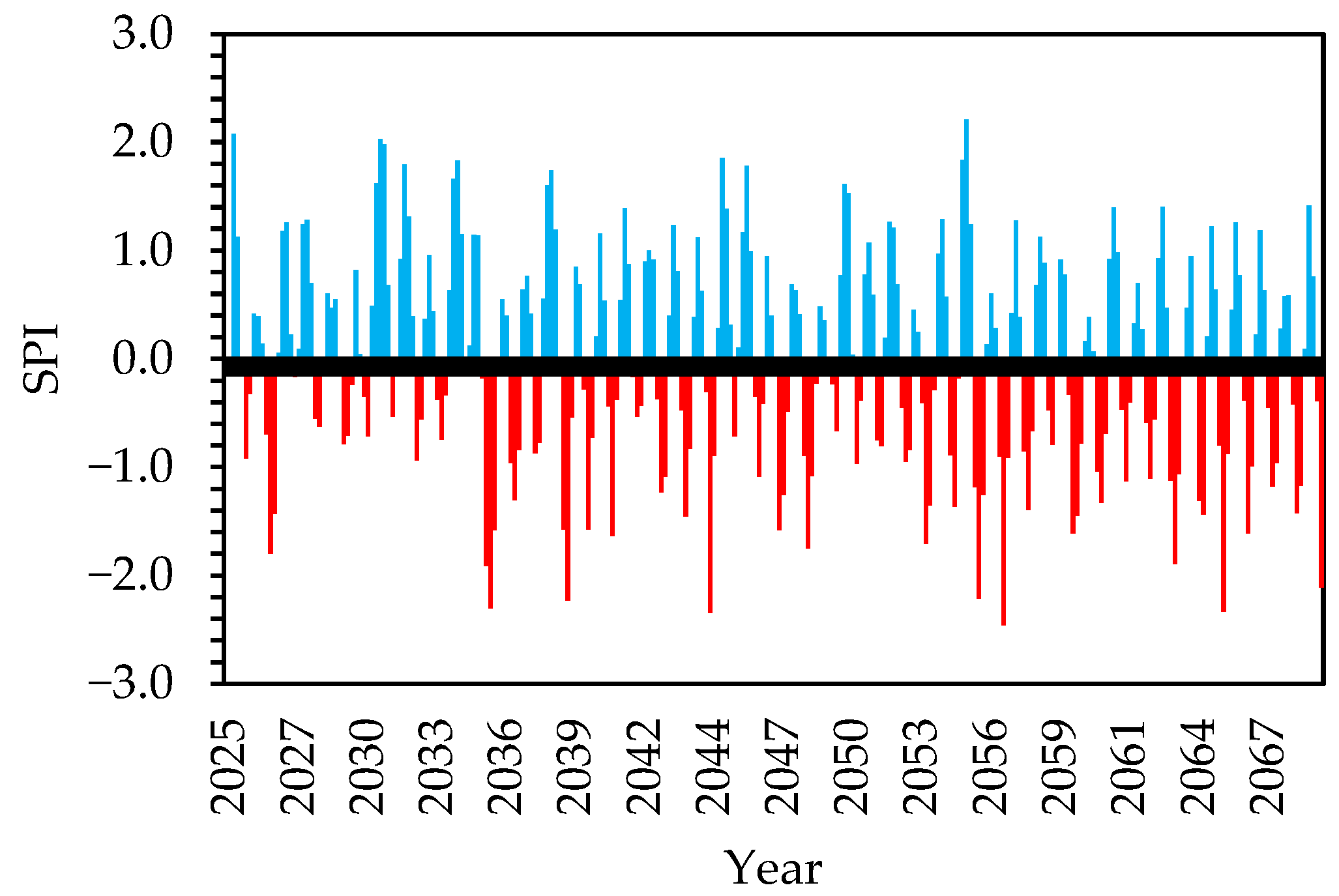
The Standardized Precipitation Index (SPI) was used to map rainfall anomalies and project drought occurrences, revealing a general increase in drought frequency. This increase can be attributed to a projected decrease in rainfall during the rainy season’s onset. RCP 8.5 projects a higher frequency of droughts than RCP 4.5, which aligns with the lower rainfall projected for the onset of the rainy season under RCP 8.5. Similar findings have been observed globally. For instance, Essa et al. [52] found that droughts in the Mediterranean region are expected to increase by at least 12% by 2060. Wu et al. [5] also projected an increase in drought prevalence across southern Africa under various global warming scenarios, and Naik and Abiodun [53] projected a higher future prevalence of droughts in the Western Cape of South Africa. The spatial distribution of drought occurrence, shown in Table 13, indicates an increase in a northeastward direction, which is consistent with historical observations by JICA [24], identifying Karonga as a drought-prone district.

Despite consistent projections of future drought prevalence, some researchers, such as Won and Kim [21], found that climate change projections did not indicate an increase in severe droughts. However, alternative drought indices, such as the Evaporative Demand Drought Index (EDDI), have projected severe droughts where SPI has not. Similar results were reported by Abiodun et al. [54], who found that SPI failed to project an increase in severe droughts across southern Africa, unlike the SPIE. This suggests that with the projected increase in average temperatures, drought prevalence may rise further in the Lufilya catchment, as drought conditions are exacerbated by extreme temperatures, low rainfall, and high relative humidity [55].

A limitation of this study is the use of SPI as the sole drought indicator, which does not fully capture drought impacts due to temperature anomalies. Other indicators, such as the EDDI, have been shown to reveal additional drought patterns not captured by SPI alone, as evidenced in southern Africa by Abiodun et al. [54]. This highlights the need for a multifaceted drought modeling approach, particularly in the Lufilya catchment, where drought conditions could worsen under high temperature and humidity. Future studies should expand this analysis by incorporating wind speed effects on soil moisture variability, to account for the comprehensive climatic impacts on drought severity.

5. Conclusions

This study examined the projected impacts of climate change on rainfall and drought prevalence in Malawi’s Lufilya catchment using an ensemble of three regional Climate Models (RCMs) and the Standardized Precipitation Index (SPI) method. The main findings reveal an increase in average daily temperatures and higher rainfall during peak wet season months under both RCP 4.5 and RCP 8.5 scenarios. However, the drier months, particularly at the onset and end of the rainy season, are projected to experience reduced rainfall, aligning with the anticipated intensification of drought conditions.

The SPI analysis indicates that drought frequency is expected to rise by the end of the century, with moderate and severe droughts becoming more prevalent under both radiative forcing scenarios. Extreme drought occurrences, in contrast, are projected to decline slightly, though this study’s focus on SPI may not fully capture temperature-induced drought impacts fully.

The insights from this study provide important applications for policymakers and water resource managers in the Lufilya catchment and broader Malawi region. Specifically, the projected trends in rainfall and drought frequency underscore the need for proactive water management strategies to mitigate the adverse effects of more frequent droughts. These findings can inform the development of early warning systems tailored to seasonal drought risks, allowing for timely agricultural interventions and water rationing during critical low-rainfall periods.

Additionally, the observed patterns of increased rainfall variability suggest the potential benefit of improving reservoir and irrigation infrastructure to optimize water storage and distribution during wetter months, thereby enhancing resilience during dry spells. Governing bodies may also consider incorporating these climate projections into long-term planning, particularly in sectors like agriculture, energy, and drinking water supply, to ensure robust climate adaptation policies.

While this study provides essential insights into projected climate change impacts on drought in the Lufilya catchment, limitations include the lack of temperature-sensitive drought indices, such as EDDI, and the exclusion of wind effects on soil moisture dynamics. Future research should include these variables to refine drought projections, providing an even stronger foundation for water management, agricultural planning, and climate adaptation efforts in the region. Addressing these aspects can further support governing bodies in implementing comprehensive drought preparedness and resilience strategies to level the effects of anticipated climate variability.

References

1. Nagarajan, R. Drought Assessment; Springer: Dordrecht, The Netherlands, 2010. [Google Scholar] [CrossRef]
2. Van Loon, A.F.; Laaha, G. Hydrological drought severity explained by climate and catchment characteristics. J. Hydrol. 2015, 526, 3–14. [Google Scholar] [CrossRef]
3. West, H.; Quinn, N.; Horswell, M. Remote sensing for drought monitoring & impact assessment: Progress, past challenges and future opportunities. Remote Sens. Environ. 2019, 232, 111291. [Google Scholar] [CrossRef]
4. Liu, Z.; Liu, S.; Ye, J.; Sheng, F.; You, K.; Xiong, X.; Lai, G. Application of a Digital Filter Method to Separate Baseflow in the Small Watershed of Pengchongjian in Southern China. Forests 2019, 10, 1065. [Google Scholar] [CrossRef]
5. Wu, G.; Chen, J.; Shi, X.; Kim, J.; Xia, J.; Zhang, L. Impacts of Global Climate Warming on Meteorological and Hydrological Droughts and Their Propagations. Earth’s Future 2022, 10, e2021EF002542. [Google Scholar] [CrossRef]
6. Hao, Z.; Singh, V. Drought characterization from a multivariate perspective: A review. J. Hydrol. 2015, 527, 668–678. [Google Scholar] [CrossRef]
7. Zhou, H.; Liu, Y. SPI Based Meteorological Drought Assessment over a Humid Basin: Effects of Processing Schemes. Water 2016, 8, 373. [Google Scholar] [CrossRef]
8. Dalezios, N.R.; Gobin, A.; Tarquis Alfonso, A.M.; Eslamian, S. Agricultural Drought Indices: Combining Crop, Climate, and Soil Factors. In Handbook of Drought and Water Scarcity, 1st ed.; Eslamian, S., Eslamian, F., Eds.; CRC Press: Boca Raton, FL, USA, 2017; pp. 73–89. [Google Scholar] [CrossRef]
9. Sun, H.; Sun, X.; Chen, J.; Deng, X.; Yang, Y.; Qin, H.; Chen, F.; Zhang, W. Different types of meteorological drought and their impact on agriculture in Central China. J. Hydrol. 2023, 627, 130423. [Google Scholar] [CrossRef]
10. Şen, Z. Assessing Wet and Dry Periods Using Standardized Precipitation Index Fractal (SPIF) and Polygons: A Novel Approach. Water 2024, 16, 592. [Google Scholar] [CrossRef]
11. Mukherjee, S.; Mishra, A.; Trenberth, K.E. Climate Change and Drought: A Perspective on Drought Indices. Curr. Clim. Change Rep. 2018, 4, 145–163. [Google Scholar] [CrossRef]
12. Khoi, D.N.; Nguyen, V.T.; Sam, T.T.; Mai, N.T.H.; Vuong, N.D.; Cuong, H.V. Assessment of climate change impact on water availability in the upper Dong Nai River Basin, Vietnam. J. Water Clim. Change 2021, 12, 3851–3864. [Google Scholar] [CrossRef]
13. Oguntunde, P.G.; Abiodun, B.J.; Lischeid, G. Impacts of climate change on hydro-meteorological drought over the Volta Basin, West Africa. Glob. Planet. Change 2017, 155, 121–132. [Google Scholar] [CrossRef]
14. Jayanthi, H.; Husak, G.J.; Funk, C.; Magadzire, T.; Chavula, A.; Verdin, J. Modeling rain-fed maize vulnerability to droughts using the standardized precipitation index from satellite estimated rainfall—Southern Malawi case study. Int. J. Disaster Risk Reduct. 2013, 4, 71–81. [Google Scholar] [CrossRef]
15. IPCC. Climate Change 2014: Synthesis Report. In Contribution of Working Groups I, II and III to the Fifth Assessment Report of the Intergovernmental Panel on Climate Change; IPCC: Geneva, Switzerland, 2014. [Google Scholar]
16. Ji, P.; Yuan, X.; Ma, F.; Pan, M. Accelerated hydrological cycle over the Sanjiangyuan region induces more streamflow extremes at different global warming levels. Hydrol. Earth Syst. Sci. 2020, 24, 5439–5451. [Google Scholar] [CrossRef]
17. Shi, X.; Chen, J.; Gu, L.; Xu, C.-Y.; Chen, H.; Zhang, L. Impacts and socioeconomic exposures of global extreme precipitation events in 1.5 and 2.0 °C warmer climates. Sci. Total Environ. 2021, 766, 142665. [Google Scholar] [CrossRef]
18. Dibaba, W.T.; Demissie, T.A.; Miegel, K. Watershed Hydrological Response to Combined Land Use/Land Cover and Climate Change in Highland Ethiopia: Finchaa Catchment. Water 2020, 12, 1801. [Google Scholar] [CrossRef]
19. Gebre, S.L.; Ludwig, F. Hydrological Response to Climate Change of the Upper Blue Nile River Basin: Based on IPCC Fifth Assessment Report (AR5). J. Climatol. Weather. Forecast. 2015, 3, 1–15. [Google Scholar] [CrossRef]
20. Mahdavi, P.; Kharazi, H.G.; Eslami, H.; Zohrabi, N.; Razaz, M. Drought occurrence under future climate change scenarios in the Zard River basin, Iran. Water Supply 2021, 21, 899–917. [Google Scholar] [CrossRef]
21. Won, J.; Kim, S. Future drought analysis using SPI and EDDI to consider climate change in South Korea. Water Supply 2020, 20, 3266–3280. [Google Scholar] [CrossRef]
22. Vincent, K. Future Climate Projections for Malawi, weADAPT. Available online: https://weadapt.org/knowledge-base/climate-services/future-climate-projections-for-malawi/ (accessed on 7 November 2024).
23. Adhikari, U.; Nejadhashemi, A. Impacts of Climate Change on Water Resources in Malawi. J. Hydrol. Eng. 2016, 21, 05016026. [Google Scholar] [CrossRef]
24. JICA, Project for National Water Resources Master Plan in the Republic of Malawi, II Vols. Ministry of Agriculture, Irrigation and Water Development (MoAIWD). 2014. Available online: https://openjicareport.jica.go.jp/pdf/12184537_08.pdf (accessed on 13 July 2024).
25. McCarthy, N.; Kilic, T.; Brubaker, J.; Murray, S.; De La Fuente, A. Droughts and floods in Malawi: Impacts on crop production and the performance of sustainable land management practices under weather extremes. Environ. Dev. Econ. 2021, 26, 432–449. [Google Scholar] [CrossRef]
26. Kelly, L.; Bertram, D.; Kalin, R.; Ngongondo, C.; Sibande, H. A National Scale Assessment of Temporal Variations in Groundwater Discharge to Rivers: Malawi. Am. J. Water Eng. 2020, 6, 1. [Google Scholar] [CrossRef]
27. FAO. CLIMWAT|Land & Water|Food and Agriculture Organization of the United Nations|Land & Water|Food and Agriculture Organization of the United Nations. Available online: https://www.fao.org/land-water/databases-and-software/climwat-for-cropwat/en/ (accessed on 5 August 2024).
28. Abeysingha, N.S.; Jayasekara, J.M.N.S.; Meegastenna, T.J. Stream flow trends in up and midstream of Kirindi Oya river basin in Sri Lanka and its linkages to rainfall. Mausam 2017, 68, 99–110. [Google Scholar] [CrossRef]
29. Dibaba, W.T.; Miegel, K.; Demissie, T.A. Evaluation of the CORDEX regional climate models performance in simulating climate conditions of two catchments in Upper Blue Nile Basin. Dyn. Atmos. Ocean. 2019, 87, 101104. [Google Scholar] [CrossRef]
30. Gadissa, T.; Nyadawa, M.; Behulu, F.; Mutua, B. The Effect of Climate Change on Loss of Lake Volume: Case of Sedimentation in Central Rift Valley Basin, Ethiopia. Hydrology 2018, 5, 67. [Google Scholar] [CrossRef]
31. Whitaker, J. netCDF4-Python: A Python Interface to the netCDF C Library. GitHub Repository. Available online: https://github.com/Unidata/netcdf4-python (accessed on 17 September 2024).
32. Di Luca, A.; Pitman, A.J.; de Elía, R. Decomposing Temperature Extremes Errors in CMIP5 and CMIP6 Models. Geophys. Res. Lett. 2020, 47, e2020GL088031. [Google Scholar] [CrossRef]
33. Wild, M. The global energy balance as represented in CMIP6 climate models. Clim. Dyn. 2020, 55, 553–577. [Google Scholar] [CrossRef]
34. Iles, C.E.; Vautard, R.; Strachan, J.; Joussaume, S.; Eggen, B.R.; Hewitt, C.D. The benefits of increasing resolution in global and regional climate simulations for European climate extremes. Geosci. Model Dev. 2020, 13, 5583–5607. [Google Scholar] [CrossRef]
35. Teutschbein, C.; Seibert, J. Bias correction of regional climate model simulations for hydrological climate-change impact studies: Review and evaluation of different methods. J. Hydrol. 2012, 456, 12–29. [Google Scholar] [CrossRef]
36. Crochemore, L.; Ramos, M.-H.; Pappenberger, F. Bias correcting precipitation forecasts to improve the skill of seasonal streamflow forecasts. Hydrol. Earth Syst. Sci. 2016, 20, 3601–3618. [Google Scholar] [CrossRef]
37. Maharjan, M.; Aryal, A.; Talchabhadel, R.; Thapa, B.R. Impact of Climate Change on the Streamflow Modulated by Changes in Precipitation and Temperature in the North Latitude Watershed of Nepal. Hydrology 2021, 8, 117. [Google Scholar] [CrossRef]
38. Valdés-Pineda, R.; Demaría, E.M.C.; Valdés, J.B.; Wi, S.; Serrat-Capdevilla, A. Bias correction of daily satellite-based rainfall estimates for hydrologic forecasting in the Upper Zambezi, Africa. Hydrol. Earth Syst. Sci. Discuss. 2016, 2016, 1–28. [Google Scholar] [CrossRef]
39. McKee, T.B.; Doesken, N.J.; Kleist, J. The relationship of drought frequency and duration to time scales. In Proceedings of the 8th Conference on Applied Climatology, Anaheim, CA, USA, 17–22 January 1993; pp. 179–183. [Google Scholar]
40. Moccia, B.; Mineo, C.; Ridolfi, E.; Russo, F.; Napolita, F. SPI-Based Drought Classification in Italy: Influence of Different Probability Distribution Functions. Water 2022, 14, 3668. [Google Scholar] [CrossRef]
41. Spinoni, J.; Naumann, G.; Carrao, H.; Barbosa, P.; Vogt, J. World drought frequency, duration, and severity for 1951–2010: World drought climatologies for 1951–2010. J. Climatol. 2014, 34, 2792–2804. [Google Scholar] [CrossRef]
42. Al-Faraj, F.A.M.; Scholz, M.; Tigkas, D.; Boni, M. Drought indices supporting drought management in transboundary watersheds subject to climate alterations. Water Policy 2015, 17, 865–886. [Google Scholar] [CrossRef]
43. Nangoma, E. National Adaptation Strategy to Climate Change Impacts: A Case Study of Malawi, Human Development Report Office, Human Development Report. 2007. Available online: https://hdr.undp.org/system/files/documents/nangomaeverhartmalawi.pdf (accessed on 24 September 2024).
44. Jasrotia, A.S.; Baru, D.; Kour, R.; Ahmad, S.; Kour, K. Hydrological modeling to simulate stream flow under changing climate conditions in Jhelum catchment, western Himalaya. J. Hydrol. 2021, 593, 125887. [Google Scholar] [CrossRef]
45. Haile, A.T.; Akawka, A.L.; Berhanu, B.; Rientjes, T. Changes in water availability in the Upper Blue Nile basin under the representative concentration pathways scenario. Hydrol. Sci. J. 2017, 62, 2139–2149. [Google Scholar] [CrossRef]
46. Chattopadhyay, S.; Edwards, D.R.; Yu, Y.; Hamidisepehr, A. An Assessment of Climate Change Impacts on Future Water Availability and Droughts in the Kentucky River Basin. Environ. Process. 2017, 4, 477–507. [Google Scholar] [CrossRef]
47. Byrne, M.; O’Gorman, A. The Response of Precipitation Minus Evapotranspiration to Climate Warming: Why the ‘Wet-Get-Wetter, Dry-Get-Drier’ Scaling Does Not Hold over Land*. J. Clim. 2015, 28, 8078–8092. [Google Scholar] [CrossRef]
48. Elshamy, M.E.; Seierstad, I.A.; Sorteberg, A. Impacts of climate change on Blue Nile flows using bias-corrected GCM scenarios. Hydrol. Earth Syst. Sci. 2009, 13, 551–565. [Google Scholar] [CrossRef]
49. Ghimire, U.; Piman, T.; Shrestha, M.; Aryal, A.; Krittasudthacheewa, C. Assessment of Climate Change Impacts on the Water, Food, and Energy Sectors in Sittaung River Basin, Myanmar. Water 2022, 14, 3434. [Google Scholar] [CrossRef]
50. Aich, V.; Liersch, S.; Vetter, T.; Huang, S.; Tecklenburg, J.; Hoffmann, P.; Koch, H.; Fournet, S.; Krysanova, V.; Müller, E.N.; et al. Comparing impacts of climate change on streamflow in four large African river basins. Hydrol. Earth Syst. Sci. 2014, 18, 1305–1321. [Google Scholar] [CrossRef]
51. Iyakaremye, V.; Zeng, G.; Yang, X.; Zhang, G.; Ullah, I.; Gahigi, A.; Vuguziga, F.; Asfaw, T.G.; Ayugi, B. Increased high-temperature extremes and associated population exposure in Africa by the mid-21st century. Sci. Total Environ. 2021, 790, 148162. [Google Scholar] [CrossRef] [PubMed]
52. Essa, Y.H.; Hirschi, M.; Thiery, W.; El-Kenawy, A.M.; Yang, C. Drought characteristics in Mediterranean under future climate change. npj Clim. Atmos. Sci. 2023, 6, 133. [Google Scholar] [CrossRef]
53. Naik, M.; Abiodun, B.J. Projected changes in drought characteristics over the Western Cape, South Africa. Meteorol. Appl. 2020, 27, e1802. [Google Scholar] [CrossRef]
54. Abiodun, B.J.; Makhanya, N.; Petja, B.; Abatan, A.A.; Oguntunde, G. Future projection of droughts over major river basins in Southern Africa at specific global warming levels. Theor. Appl. Climatol. 2019, 137, 1785–1799. [Google Scholar] [CrossRef]
55. Ullah, I.; Mukherjee, S.; Syed, S.; Mishra, A.K.; Ayugi, B.O.; Aadhar, S. Anthropogenic and atmospheric variability intensifies flash drought episodes in South Asia. Commun. Earth Environ. 2024, 5, 267. [Google Scholar] [CrossRef]
Figure 1. Lufilya River catchment.
Water 16 03548 g001
Figure 2. Q-Q plot of observed rainfall data for Lufilya catchment.
Water 16 03548 g002
Figure 3. Q-Q plot of simulated rainfall data of CCLM4-8-17 model for Lufilya catchment.
Water 16 03548 g003
Figure 4. Q-Q plot of simulated rainfall data of RCA4 model for Lufilya catchment.
Water 16 03548 g004
Figure 5. Q-Q plot of simulated rainfall data of REMO2009 model for Lufilya catchment.
Water 16 03548 g005
Figure 6. Monthly average change in precipitation for CCLM4-8-17 model under (RCP4.5).
Water 16 03548 g006
Figure 7. Monthly average change in precipitation for CCLM4-8-17 model under (RCP8.5).
Water 16 03548 g007
Figure 8. Monthly average change in precipitation for REMO2009 model under (RCP4.5).
Water 16 03548 g008
Figure 9. Monthly average change in precipitation for REMO2009 model under (RCP8.5).
Water 16 03548 g009
Figure 10. Monthly average change in precipitation for RECA model under (RCP4.5).
Water 16 03548 g010
Figure 11. Monthly average change in precipitation for RECA model under (RCP8.5).
Water 16 03548 g011
Figure 12. Variations in average temperature for CCLM4-8-17 model under (RCP4.5).
Water 16 03548 g012
Figure 13. Variations in average temperature for CCLM4-8-17 model under (RCP8.5).
Water 16 03548 g013
Figure 14. Variations in average temperature for REMO2009 model under (RCP4.5).
Water 16 03548 g014
Figure 15. Variations in average temperature for REMO2009 model under (RCP8.5).
Water 16 03548 g015
Figure 16. Variations in average temperature for RCA4 model under (RCP8.5).
Water 16 03548 g016
Figure 17. Variations in average temperature for RCA4 model under (RCP8.5).
Water 16 03548 g017
Figure 18. Temporal variations in SPIs, Historical (1976–1999).
Water 16 03548 g018
Figure 19. Temporal variations in SPIs, Historical (2000–2022): Where the red spikes means drought occurrence while the blue ones means no drought occurrence.
Water 16 03548 g019
Figure 20. Temporal variations in SPIs, RCP 4.5 (2025–2069): Where the red spikes means drought occurrence while the blue ones means no drought occurrence.
Water 16 03548 g020
Figure 21. Temporal variations in SPIs, RCP 4.5 (2070–2100): Where the red spikes means drought occurrence while the blue ones means no drought occurrence.
Water 16 03548 g021
Figure 22. Temporal variations in SPIs, RCP 8.5 (2025–2069): Where the red spikes means drought occurrence while the blue ones means no drought occurrence.
Water 16 03548 g022