An Adaptive Process-Wise Fitting Approach for Hydrological Modeling Based on Streamflow and Remote Sensing Evapotranspiration

Abstract

Modern hydrological modeling frequently incorporates global remote sensing or reanalysis products for multivariate calibration. Although these datasets significantly contribute to model accuracy, the inherent uncertainties in the datasets and multivariate calibration present challenges in the modeling process. To address this issue, this study introduces an adaptive, process-wise fitting framework for the iterative multivariate calibration of hydrological models using global remote sensing and reanalysis products. A distinctive feature is the “kinship” concept, which defines the relationship between model parameters and hydrological processes, highlighting their impacts and connectivity within a directed graph. The framework subsequently develops an enhanced particle swarm optimization (PSO) algorithm for stepwise calibration of hydrological processes. This algorithm introduces a learning rate that reflects the parameter’s kinship to the calibrated hydrological process, facilitating efficient exploration in search of suitable parameter values. This approach maximizes the performance of the calibrated process while ensuring a balance with other processes. To ease the impact of inherent uncertainties in the datasets, the Extended Triple Collocation (ETC) method, operating independently of ground truth data, is integrated into the framework to assess the simulation of the calibrated process using remote sensing products with inherent data uncertainty. This proposed approach was implemented with the SWAT model in both arid and humid basins. Five calibration schemes were designed and evaluated through a comprehensive comparison of their performance in three repeated experiments. The results highlight that this approach not only improved the accuracy of ET simulation across sub-basins but also enhanced the precision of streamflow at gauge stations, concurrently reducing parameter uncertainty. This approach significantly advances our understanding of hydrological processes, demonstrating the potential for both theoretical and practical applications in hydrology.

1. Introduction

The increasing accessibility of global hydrological remote sensing and reanalysis products [1] has significantly shifted hydrological model calibration away from traditional univariate methods, which rely solely on gauged stream data [2]. This shift has spurred a notable trend of moving towards the broader adoption of multivariate approaches [3,4]. However, despite these advancements, uncertainties are introduced by remote sensing and reanalysis products, often containing unknown errors [5,6]. In addition, parameter uncertainties stemming from inadequate representations of hydrological processes within multivariate approaches [7,8] further complicate the situation. Developing effective calibration strategies is crucial to mitigating these uncertainties, particularly when using remote sensing or reanalysis products with inherent data errors [9,10].

Hydrological remote sensing and reanalysis products, such as those for evapotranspiration (ET) and soil moisture [1,11,12,13], are increasingly utilized as substitutes for ground observations in multivariable calibration in ungauged areas, attributed to their extensive spatial coverage, broad temporal span, and accessibility of data sources [14,15,16]. However, it is crucial to recognize that these datasets can exhibit significant biases and random errors at local levels [17], which may lead to overestimations or underestimations of physical variables. Moreover, the absence of ground truth values makes these errors difficult to detect, presenting significant risks to hydrological modeling [18,19]. To intelligently address data with inherent uncertainties, the Extended Triple Collocation (ETC) evaluation scheme [20] has gained prominence. This method is notably used to assess the accuracy of remote sensing products like ET and soil moisture [21,22,23] and stands out for its ability to estimate the determination coefficient and the standard error of random errors from three datasets without requiring ground truth in environmental modeling [24]. The ETC’s capacity to map the spatial distribution of these bias-insensitive metrics provides an insightful approach to navigating and mitigating data uncertainties.

In multivariate calibration, neglecting the differential impacts of parameters on various hydrological processes often leads to an improper representation of the physical characteristics of model parameters, thus posing significant challenges in managing parameter uncertainty [25,26]. By integrating different scenarios, such as streamflow, evapotranspiration (ET), and soil moisture, and applying weighted averaging or streamflow-dominated weight allocation schemes, the issue of model equifinality within hydrological systems can be alleviated [25,27,28,29]. It has been observed that this integration can sometimes result in a varied reduction in the accuracy of streamflow predictions [30,31], contrary to the goal of improving predictions across all variables. This issue becomes particularly evident when examining two popular multivariate calibration methods. Joint calibration often fails to account for the sensitivity of parameters to different hydrological processes, which can result in distortions and deviations from the true physical meanings of parameters during iterative calibration [14,32]. Conversely, stepwise calibration aims to reduce the distortion caused by joint calibration [25]; however, strictly binding parameters to specific hydrological processes can neglect their effects on other processes. Additionally, not using a universal parameter set throughout the calibration process can confound the influence of parameters on the objective function [5,15,33]. These challenges fundamentally arise from disregarding the differential impacts of parameters on various hydrological processes [34]. In other words, some parameters affect a single process, while others may impact multiple processes, often interacting within the same system and thereby leading to parameter uncertainty [11,15,31]. Therefore, a key consideration in parameter iteration during multivariate calibration is to ensure that adjustments are made only for relevant hydrological processes, thus maximizing their role in their respective processes and maintaining the consistency of physical properties with real-world conditions. However, finding a universally accepted solution to achieve this goal remains a challenge with current calibration methods [3,35,36].

Therefore, to mitigate the impact of uncertainties in remote sensing products on the multivariate calibration of hydrological models, this study develops an adaptive stepwise fitting framework based on enhanced particle swarm optimization (PSO). This framework emphasizes the parametrization of model parameters according to their relevant hydrological processes through an iterative calibration approach. The main features of the framework are as follows: (1) The use of Extended Triple Collocation (ETC) to estimate bias-insensitive metrics of remote sensing products without relying on ground truth data. This allows for the incorporation of remote-sensing-based evapotranspiration to assess SWAT model outputs, thereby reducing the impact of input uncertainties on model performance. (2) The construction of a directed graph representing the relationships between hydrological processes, where inputs and outputs are mapped and a hierarchy of “kinship” is established between different hydrological processes and their associated parameters. This framework evaluates hydrological processes using both remote sensing products and streamflow data, while simultaneously updating relevant parameters based on their “kinship” weight values related to the processes, ensuring that parameters are only adjusted according to closely related processes and avoiding unnecessary adjustments to distant ones.

2. Study Areas and Methods

2.1. Study Areas

The Malian Basin, located in the Loess Plateau of China, covers an area of 2994 km² and spans from 35°3′ to 36°55′ N latitude and 107°30′ to 108°16′ E longitude (see Figure 1). The basin stretches approximately 100 km from north to south and features typical Loess Plateau terrain, including loess hills, ridges, and tablelands, extending from the upstream northern area to the downstream southern region. The dominant land cover types in the Malian Basin are grasslands (64.92%), croplands (18.06%), and forests (7.79%), with limited forested areas mainly found in the southeastern part of the basin [37,38]. The region experiences an arid to semi-arid climate, with annual precipitation ranging from about 400 mm in the upstream to approximately 600 mm in the downstream. Most of the rainfall occurs between June and September, exhibiting strong seasonal variation. Interannual precipitation variability is significant, with wet years accumulating up to two to three times the precipitation of drought years [39].

The Meichuan Basin, situated in the upper Gan River region of Jiangxi Province, covers an area of 6341 km² and is located between 26°00′ and 27°09′ N latitude and between 115°36′ and 116°38′ E longitude (see Figure 2). The basin features undulating low and mid-level mountains, with elevations ranging from 137 to 1425 m, and its primary outflow is monitored at the Fenkeng hydrological station. The main land cover types are forests (67.02%), croplands (13.55%), and grasslands (13.05%). The basin has mild temperatures, averaging 17 °C annually, with winter temperatures above 0 °C and summer peaks around 25 °C. Annual precipitation averages 1628 mm, primarily concentrated in the summer months. The basin maintains a high average relative humidity of over 80%, contrasting significantly with the arid conditions of the Malian Basin.

2.2. Methods

Hydrological models encompass various physical processes, necessitating that outputs from processes with observational data closely align with those observations during calibration. However, optimization should not be confined to these processes alone but should extend across all model parameters [40].

We propose an adaptive, process-wise fitting framework (APWF) for hydrological model calibration. This framework integrates observed streamflow data and remote sensing evapotranspiration (ET) data, both of which are characterized by significant uncertainties, as reference datasets for multivariable calibration (Figure 3). Unlike traditional multivariable calibration methods, this framework conceptualizes the hydrological model as a directed graph. In this graph, nodes represent key physical processes, such as plant growth, evapotranspiration, and surface runoff, with each node serving as a core module within the hydrological system. Each node contains specific parameters and regulates the relationships between parameters and processes through “kinship”, ensuring rational parameter updates and thus enhancing model performance. Specifically, kinship comprises two main aspects:

1. Input–Output Relationships: Each hydrological process node contains specific parameters and is responsible for receiving input variables and generating output variables. In this framework, each node can accept outputs from other nodes as inputs, with the resulting calculations becoming inputs for downstream nodes. This flow of inputs and outputs not only reflects the intrinsic logic of individual hydrological processes but also illustrates the interdependencies among various processes. For example, the input for a given node may come from multiple upstream processes (e.g., precipitation, evapotranspiration, soil moisture), while the output of that node serves as an input for other downstream processes (e.g., streamflow, runoff). The structured and orderly nature of these input–output relationships allows us to clearly capture the interactions among different hydrological processes.

2. Topological Relationships and “Hop Distance”: In addition to the input–output relationships, the second aspect of kinship involves the topological relationships of hydrological process nodes within the directed graph. We define kinship by analyzing the “hop distance” between the current node and its preceding nodes. This means that influences between nodes are not just direct, but can also propagate indirectly through multiple intermediary nodes. Nodes with a shorter hop distance exhibit stronger associations, while those further apart have a weaker influence. Therefore, each node in the framework takes into account not only direct influences but also indirect impacts through topological paths, adjusting the parameter update strategy accordingly. This topological dependence helps in reasonably distributing the magnitude of parameter adjustments during the model calibration process.

Moreover, the framework supports flexible stepwise calibration, allowing for the use of different evaluation metrics tailored to the quality of diverse reference data.

The calibration process in this framework unfolds as follows:

1. Candidate Solution Generation: Initial solutions are generated using Monte Carlo sampling, providing a diverse pool of potential solutions. An optimal solution will finally be selected through iterative calibration by refining the parameters step by step as below.

2. Candidate Solution Evaluation: Candidate solutions are evaluated on a process-by-process basis. Processes with outputs that have corresponding ground truth observations are assessed using standard metrics, such as KGE. For processes where outputs are compared to reference data from remote sensing with inherent uncertainty, specific methods, like the ETC method, are used for evaluation.

3. Parameter Refinement: Parameter adjustments are made via particle swarm optimization (PSO) with variable learning rates, determined by the “kinship” between the parameter and the process being calibrated. Parameters directly linked to the calibrated process are adjusted in larger steps for accelerated convergence, while those associated with more distant processes are updated in smaller steps for finer tuning. This approach ensures efficient and targeted calibration.

4. Iterative Fitting: The calibration iterates through the above evaluation and refinement steps, sequentially addressing each process defined by the directed graph until simulated process outputs show minimal deviation from observations.

This comprehensive approach ensures a nuanced understanding of hydrological dynamics, effectively addressing the unique challenges presented by integrating diverse data sources into hydrological modeling. By incorporating both ground truth and remote sensing data with varying levels of uncertainty, the framework enhances model accuracy and reliability across different hydrological processes.

2.3. Modeling Hydrological System Using Directed Graphs

2.3.1. Graph-Based Representation of Hydrological Processes and Interdependencies

Graph-based models are instrumental not only in illustrating the interconnectedness of water bodies and the movement of water and pollutants but also in providing a comprehensive framework to capture the intricate interrelations among the diverse physical processes that make up a hydrologic system [41]. In this study, we constructed a directed graph based on the widely applied distributed hydrological model, the Soil and Water Assessment Tool (SWAT). By leveraging the inherent interdependencies among physical processes defined in SWAT, such as precipitation, plant growth, evapotranspiration, soil water dynamics, surface runoff (SCS), groundwater interactions, and channel routing, we conceptualized a directed graph system [16,42,43]. In this representation, each node symbolizes a distinct physical process, while the edges denote the associations between nodes, dictated by their interlinked inputs or outputs (Figure 4).

In the graph representation of the hydrological system, parameters are assigned to individual physical processes they directly influence. During the calibration of an active node (process), the parameters associated with that node are assumed to have a significant influence on its behavior. In contrast, nodes further along the back-propagation pathway have a diminishing impact on the active node, highlighting the importance of proximity in defining the strength of parameter–process relationships within the hydrological modeling framework. This approach emphasizes the local influence of parameters on processes, ensuring that calibration is both targeted and efficient.

2.3.2. Quantifying Parameter Influences on Hydrological Processes

A hydrological model comprises a critical set of physical parameters used to characterize the spatio-temporal aspects of hydrological processes [44]. Conventionally, multivariate calibration aimed at parameter inversion typically involves an exhaustive approach [45]. This process begins by generating a set of initial candidate solutions, followed by evaluating model outputs and adjusting parameter values for each candidate in an attempt to achieve optimal calibration. However, this method treats all parameters equally during the adjustment phase. As noted in Section 2.3.1, these parameters do not exert a uniform influence on the processes, which can lead to inefficiencies in the calibration process.

Based on the directed graph illustrating process interdependencies (Figure 4) and parameter–process associations, we established parameter–process relationships. Parameters were categorized into four groups based on the hop distance of the process directly influenced by the parameter to the currently calibrated process in the graph:

• Strong Association: Solely related to the currently calibrated process, with no links to any preceding processes in the graph.
• Moderate Association: Not related to the currently calibrated process but associated with its preceding processes.
• Weak Association: Related to both the currently calibrated process and preceding processes.
• Unrelated: No relation to any preceding or current processes.

Therefore, the parameter learning rates constructed in this study were initially determined based on the “kinship” relationships within the directed graph and the parameter sensitivities. These relationships helped assess the relative importance of each parameter to the hydrological process being calibrated, rather than relying on absolute values. Subsequently, the relative relationships were refined through repeated experiments until excellent results were achieved in both study areas. Ultimately, the parameter learning rates corresponding to the parameter correlations in this study were tentatively set as strong (2), moderate (1.5), weak (0.5), and unrelated (0).

2.4. Process-Specific Simulation Evaluation Using Data with Inherent Uncertainties

In evaluating the outputs of physical processes in a hydrological system, two distinct methods are employed, each depending on the quality of observations (or reference data):

(1) For processes evaluated using ground truth data, conventional metrics, including Kling–Gupta Efficiency (KGE), Nash–Sutcliffe Efficiency Coefficient (NSE), coefficient of determination (R2), and Percent Bias (PBIAS) are employed [10].

To compare the performance of simulated variables against truth values, we employed the Kling–Gupta Efficiency index. The KGE is a prevalent and comprehensive performance metric in the assessment of hydrological modeling [1], incorporating three key components: CC (the linear correlation between simulated and observed values), beta (the bias ratio between the mean of the simulated and observed values), and gamma (the variability ratio between the standard deviations of the simulated and observed values) [46].

$$CC={\displaystyle \frac{{\displaystyle {\sum }_{j=1}^n(S_j-S_{mean})\left(O_j-O_{mean}\right)}}{\sqrt{{\displaystyle {\sum }_{j=1}^n{(S_j-S_{mean})}^2}}\sqrt{{\displaystyle {\sum }_{j=1}^n{(O_j-O_{mean})}^2}}}}$$

(1)

$$Beta={\displaystyle \frac{{\mu }_S}{{\mu }_O}}$$

(2)

$$Gamma={\displaystyle \frac{{\sigma }_S}{{\sigma }_O}}$$

(3)

$$KGE=1-\sqrt{{(1-CC)}^2+{(1-Beta)}^2+{(1-Gamma)}^2}$$

(4)

where $S$ and $O$ are the observed and simulated values, while ${\mu }_S$ and ${\mu }_O$ represent their respective means, and ${\sigma }_S$ and ${\sigma }_O$ are the standard deviations of the observed and simulated values.

In addition, this study quantified the stability of the output results based on the 95% prediction uncertainty band (95PPU) [47], calculated at the 2.5% and 97.5% levels of the cumulative distribution function of the output variable’s evaluation results. The specific formula is as follows:

$$P={\displaystyle \frac{1}{k}}{\displaystyle \sum _{t-1}^k{(X_U-X_L)}_t}$$

(5)

In the formula, $k$ is the number of observed data points, which refers to the quantity of observed data within the time step. $X_U$ and $X_L$ represent the upper and lower boundaries of the 95PPU, respectively.

$$R={\displaystyle \frac{P}{{\sigma }_{obs}}}$$

(6)

${\sigma }_{obs}$ stands for the standard deviation of the observation data. After completing the calculation, the quality of calibration and predictive uncertainty can be assessed based on the closeness of $P$ to 1 (i.e., all observations encompassed by the prediction uncertainty should be greater than 0.7) and $R$ to 1 (i.e., achieving a small uncertainty band).

(2) For processes assessed using data with inherent uncertainties from external model sources, the Extended Triple Collocation (ETC) method by McColl et al. (2014) is applied. This technique allows for the assessment of uncertainty in process simulations in the absence of ground truth values. It has been proven to be highly significant in mitigating model errors caused by input uncertainties [21,22,23].

Given three simulated variables X_i (i ∈ (1, 2, 3)) that are linearly related to the true value T, each with an additive random error εi, respectively, the standard deviation of the random errors for the three variables can be estimated using the ETC method. The estimation of uncertainties of the three simulations is based on several assumptions: (1) a linear correlation between the simulations and their corresponding true values; (2) stability of errors over time, without temporal variation; (3) independence of errors across the three simulations; and (4) independence of errors in the simulations from the true values.

The linear expression of the simulated variable and the true variable T is as follows:

$${\mathrm{X}}_i={\alpha }_i+{\beta }_{i}T+{\epsilon }_i\begin{array}{cc}& \end{array}(i=1,2,3)$$

(7)

where X_i represents the i-th simulated variable, α_i and β_i are the intercept and slope parameters, respectively, and ε_i is the random error.

$$Q_{ij}=Cov(X_i,X_j)=E(X_i,X_j)-E(X_i)E(X_j)$$

(8)

where Q_ij represents the covariance between the variables X_i and X_j.

$$Stderr=\left[\begin{array}{c}\sqrt{Q_{11}-{\displaystyle \frac{Q_{12}{Q}_{13}}{Q_{23}}}}\\ \sqrt{Q_{22}-{\displaystyle \frac{Q_{12}{Q}_{23}}{Q_{13}}}}\\ \sqrt{Q_{33}-{\displaystyle \frac{Q_{13}{Q}_{23}}{Q_{12}}}}\end{array}\right]$$

(9)

$$Rho=\pm \left[\begin{array}{c}\sqrt{{\displaystyle \frac{Q_{12}{Q}_{13}}{Q_{11}{Q}_{23}}}}\\ sign(Q_{13}{Q}_{23})\sqrt{{\displaystyle \frac{Q_{12}{Q}_{23}}{Q_{22}{Q}_{13}}}}\\ sign(Q_{12}{Q}_{23})\sqrt{{\displaystyle \frac{Q_{12}{Q}_{23}}{Q_{33}{Q}_{12}}}}\end{array}\right]$$

(10)

where Stderr is the standard deviation of the random errors of the i-th simulated variable, and Rho is the correlation coefficient of the variable; consequently, the coefficient of determination can be obtained by squaring Rho. They both can serve as indicators for ranking the variables simulated by physical processes in the hydrological model.

2.5. Parameter Updating by Improved PSO with Learning Rates

PSO is a machine learning method that optimizes problems through iterative attempts to improve candidate solutions based on a given quality metric [48]. It accomplishes this by maintaining a set of candidate solutions, referred to as particles, and guiding their movement within the search space using mathematical formulas based on particle positions and velocities [49]. Importantly, each particle’s movement is influenced by its best-known local position (pbest) and is also guided towards the best-known global position (gbest) within the search space, which is dynamically updated as other particles find superior positions.

In hydrological modeling, the calibration of gbest and pbest is not solely dependent on their current positions and velocities; it also hinges on their alignment with the actual values of the system’s physical processes. Based on the level of alignment, the model is evaluated using the ETC method and other conventional metrics such as KGE, NSE, and R2, as outlined in Section 2.4. PSO excels in navigating complex spaces to efficiently identify high-performance parameter sets, contrasting with traditional methods such as random sampling or stratified sampling methods like Latin Hypercube Sampling (LHS) [50] and Sobol’ sequences [51], which are effective mainly in low-dimensional cases but fail to locate optimal values in high-dimensional scenarios [52]. PSO suggests new candidate parameter sets based on information gathered from previously explored parameter sets. The sampled parameter values exhibit clear support for values around the best-known positions. This algorithm focuses on promising regions and makes better use of candidate solutions to search for optimal solutions in high-dimensional solution spaces [52].

The key steps of PSO for hydrological modeling are outlined below:

(1). Initialize a group of particles within the parameter space. Initialize their velocities and positions, and set each individual’s current position as the local best—pbest, while the best individual in the particle swarm becomes the current global best—gbest.

(2). In each iteration, particles update themselves by moving toward the directions of pbest and gbest. With each position update, the fitness function of a particle is computed, and pbest and gbest positions are updated based on fitness value comparisons.

(3). If a particle’s current fitness function value is better than its pbest value, the pbest is replaced by the current position.

(4). If a particle’s pbest value is better than the gbest, the gbest is replaced by the pbest of the particle.

(5). The velocities (${V_i}^n$) and positions (X_i) of the i-th particle are updated at the n-th iteration according to the following formulas, where ω is the weight factor, c₁ and c₂ are local and global learning factors, and r₁ and r₂ are random numbers in [0, 0.5].

$$V_{i,j}^{n+1}=\omega \cdot V_{i,j}^n+c_1{r}_1(P_{i,j}^{pbest}-X_{i,j})+c_2{r}_2(P_j^{gbest}-X_{i,j})$$

(11)

However, heuristic algorithms like PSO often fail to adequately consider parameter sensitivity. Neglecting the relationship between parameters and target variables during the parameter iteration process can often be fatal. Therefore, in this study, we introduced parameter learning rates to control the iteration rates of different parameters in various hydrological processes, in addition to the formulas mentioned above.

$$V_{i,j}^{n+1}=W_{k,j}[\omega \cdot V_{i,j}^n+c_1{r}_1(P_{i,j}^{pbest}-X_{i,j})+c_2{r}_2(P_j^{gbest}-X_{i,j})]$$

(12)

where the weight, denoted as W_k,j, is newly introduced to reflect the impact of the j-th parameter on the physical process outputting the k-th variable within the graph-based hydrological system. It serves as a learning rate.

Theoretically, the learning rate range is [0, 2]. This value is contingent on parameter categories. Empirically, default values are assigned as follows: 2 for strong, 1.5 for moderate, 0.5 for weak, and 0 for unrelated. In this categorization, a weight of 0 implies that the parameter will not be updated in the current process calibration.

(6). Determine whether the termination condition has been reached. The method iteratively searches for the optimal solution (see Figure 5). For calibration involving our proposed ETC-estimated metrics, the iteration continues until the difference in the ranking scores of all process outputs becomes statistically insignificant (via Cohen’s d [53]) compared to the best results obtained from previous iterations, and the evaluation function reaches a threshold, such as the correlation coefficient exceeding 0.8. For calibrations using only traditional metrics, such as the Kling–Gupta Efficiency (KGE), the iteration halts when the difference becomes statistically insignificant and the optimal solution value exceeds a specified threshold for the metric in question (e.g., KGE should be greater than 0.5).

2.6. Experimental Design

2.6.1. Experimental Setup

The experiment aimed to evaluate the two designs outlined in Section 2.4 and Section 2.5, assessing whether they represent improvements over existing calibration methods and ensuring a parameter set capable of satisfying all observed variable processes. This involved (1) a novel method for ranking model outputs using data with inherent uncertainties; and (2) the use of process–process relationships to guide parameter update strategies across all processes in the hydrological system. To fairly showcase the characteristics of our proposed calibration method, this study designed five comparative analysis schemes in two distinctly different study areas, with fixed initial solutions, and conducted three repeated experiments (E-1, E-2, and E-3) to minimize errors caused by sampling randomness. Scheme 1 (S1) integrates observed streamflow data with inherent uncertainties and evapotranspiration (ET) products into the APWF calibration framework for stepwise calibration. It employs different evaluation methods for streamflow (KGE) and ET (ETC), adjusting iteration rates based on the correlation between parameters and their corresponding processes. In contrast, Scheme 2 (S2) treats both streamflow and GLASS ET data as ground truth, using a stepwise calibration approach. It classifies parameters into two categories based on their sensitivity and relationship with subprocesses, calibrating both outlet streamflow and sub-basin-scale ET. Scheme 3 (S3) also employs a stepwise calibration method, but the observed ET data are derived from the PMLv2 product. Scheme 4 (S4) treats streamflow and GLASS ET data as ground truth and uses a joint calibration method, calibrating both streamflow and ET with the same parameter set, with the final objective function derived from the weighted average of streamflow and ET functions. Scheme 5 (S5) also uses joint calibration, with the observed ET data coming from PMLv2. To further ensure fairness across all experiments, this study used a Cohen’s d value greater than 0.33 as the criterion for stopping iterations, ensuring that the number of iterations remained consistent across all schemes. It is worth noting that data from 2008 to 2018 were used as inputs for each scheme, with 2008 and 2009 serving as the model spin-up period, and 2010 to 2018 designated as the calibration period. To further validate the method, we used S2, which had the highest data quality and a good performance (excluding S1), as the control group. Holdout cross-validation was conducted using daily data from the Malian and Meichuan Basins. In this setup, the period from 2010 to 2015 was used for model calibration, while 2016 to 2018 was used for validation. Detailed results are provided in the Supplementary Materials, Section S3.

During the evaluation phase of the experiment, the model outputs from Scheme 1 to Scheme 5 were subjected to a standardized analysis of accuracy and uncertainty. For streamflow, this included analyzing the accuracy differences and stability of observed and best simulated streamflow using the KGE as well as the P factor and R factor. Additionally, the accuracy of the top ten solutions for each scheme converged to a specific value as the number of iterations increased. For ET, the analysis first compared the spatial distribution and magnitude of the average ET values at the sub-basin scale across three repeated experiments, exploring the model’s uncertainty. At the same time, the model’s simulated ET data, derived from remote sensing reference products, were compared with ground truth observations to assess whether the APWF framework effectively mitigates the impact of reference data biases. Subsequently, the accuracies of the best simulated ET results for each scheme and the overall simulated ET results were compared using the ETC evaluation method.

2.6.2. Parameter–Process Relations

Referring to the SWAT theoretical documentation and hydrological modeling research in arid, semi-arid, and humid regions [54,55,56,57], we empirically selected a specific set of parameters as candidates. A sensitivity analysis, following Morris, was then conducted to identify parameters sensitive to hydrological processes in our study. This analysis, aligned with SWAT documentation, helped link these parameters to their specific processes, establishing clear parameter–process relationships, as depicted in Figure 4. The findings, summarized in Table S1 in the Supplementary Materials, highlight the relatively important parameters for the SWAT model calibration process, forming a candidate parameter set closely associated with the corresponding hydrological processes. Through Morris sensitivity analysis across various study areas, we were able to discard redundant parameters, creating the initial parameter set for the actual calibration process.

2.7. Experimental Data

Table 1. The data used for hydrological modeling in the Malian Basin.

Type	Resolution	Source
Observed Streamflow	Daily (2006–2018)	Chinese Hydrological Yearbook
Observed ET	Daily (2006–2018)	China national agro-ecosystem databases Changwu station
Climate	Daily (2006–2018)	CMADS https://www.cmads.org/, accessed on 15 April 2023
ET	500 m/1 km (2006–2018)	PMLv2, GLASS https://data.tpdc.ac.cn, accessed on 20 August 2022 http://www.glass.umd.edu/, accessed on 24 August 2022
DEM	30 m	ASTER GDEM https://lpdaac.usgs.gov/products/ast14demv003/, accessed on 10 October 2022
Land Use	10 m	ESA WorldCover https://esa-worldcover.org/en, accessed on 15 October 2022
Soil	1 km	1:1,000,000 soil type map https://www.resdc.cn/Default.aspx, accessed on 10 March 2023
	30 m	China high-resolution national soil attribute dataset http://soil.geodata.cn, accessed on 21 March 2023

provides an overview of the data used in Study Area 1. During the model construction process, hydrological observation results from the “Jiaqiao” station in the “Hydrological Yearbook” were adopted as the source of observed streamflow data. These data had significant foundational value, offering reliable support for the model. Moreover, this study also gathered global remote sensing ET sensor products with higher spatial resolutions (GLASS, PMLv2), which provided accurate ET information and crucial output parameters for the model. Additionally, to highlight the tolerance of the model developed in this study to data errors, the PMLv2 data used were not the latest version, and their quality in southern China was not optimal. Furthermore, the “Changwu” ecological station near the study area was used to assess the accuracy of GLASS and PMLv2 products in the Malian Basin based on ET observation data. For watershed delineation, this study utilized the 30 m Global Digital Elevation Model (GDEM), which provides detailed information on terrain and landforms, aiding in the accurate determination of river watershed boundaries and topographic characteristics. Based on GDEM data, nine sub-watersheds were delineated, considering topographic features and water flow paths, which is beneficial for hydrological simulation and prediction. Meteorological data were obtained from the China Meteorological Assimilation Driving Datasets for the SWAT model (CMADS), offering a high spatial and temporal resolution, including accurate weather information like rainfall, temperature, and humidity, thus providing key input parameters for the model. Land use data were sourced from ESA WorldCover, providing global land cover information including forests, grasslands, urban areas, farmlands, etc., thereby offering important land use type information for the model. The national soil dataset, published by the National Earth System Science Data Center, contains soil properties such as types, texture, and organic matter contents across China, which provided vital soil parameters for the model.

For Study Area 2, the DEM data were sourced from the 30 m × 30 m resolution ASTER GDEM product provided by the International Science Data Service Platform. The land use data were obtained from the 10 m resolution FROM-GLC land use type map provided by the team of Peng Gong at Tsinghua University, which was then cropped to produce the land use type map for the Meichuan Watershed. Since the original land use types differed from those required by the SWAT model, it was necessary to reclassify and encode the land use data of the study area to generate the land use type map needed for the SWAT model. The soil data were derived from the 1:1,000,000 soil type map provided by the Resource and Environment Science and Data Center of the Chinese Academy of Sciences. Considering the lower spatial resolution of the soil type data, this study performed fuzzy clustering interpolation on the soil type attribute data to achieve a resolution of 30 m. The streamflow data for the Fenkeng station, located at the watershed outlet, were obtained from the “Yangtze River Basin Hydrological Yearbook”. The meteorological data, like in Study Area 1, were also sourced from CMADS. ET observation data near the study area were collected from the “Qianyanzhou” ecological station, as detailed in

Table 2. The data used for hydrological modeling in the Meichuan Basin.

Type	Resolution	Source
Observed Streamflow	Daily (2006–2018)	Yangtze River Basin Hydrological Yearbook
Observed ET	Daily (2006–2018)	China national agro-ecosystem databases Qianyanzhou station
Climate	Daily (2006–2018)	CMADS https://www.cmads.org/, accessed on 15 April 2023
ET	500 m/1 km (2006–2018)	PMLv2, GLASS https://data.tpdc.ac.cn, accessed on 20 August 2022 http://www.glass.umd.edu/, accessed on 24 August 2022
DEM	30 m	ASTER GDEM https://lpdaac.usgs.gov/products/ast14demv003/, accessed on 10 October 2022
Land Use	10 m	FROM-GLC https://data-starcloud.pcl.ac.cn/zh, accessed on 22 October 2022
Soil	1 km	1:1,000,000 soil type map https://www.resdc.cn/Default.aspx, accessed on 10 March 2023
	30 m	China high-resolution national soil attribute dataset http://soil.geodata.cn, accessed on 21 March 2023

.

3. Results

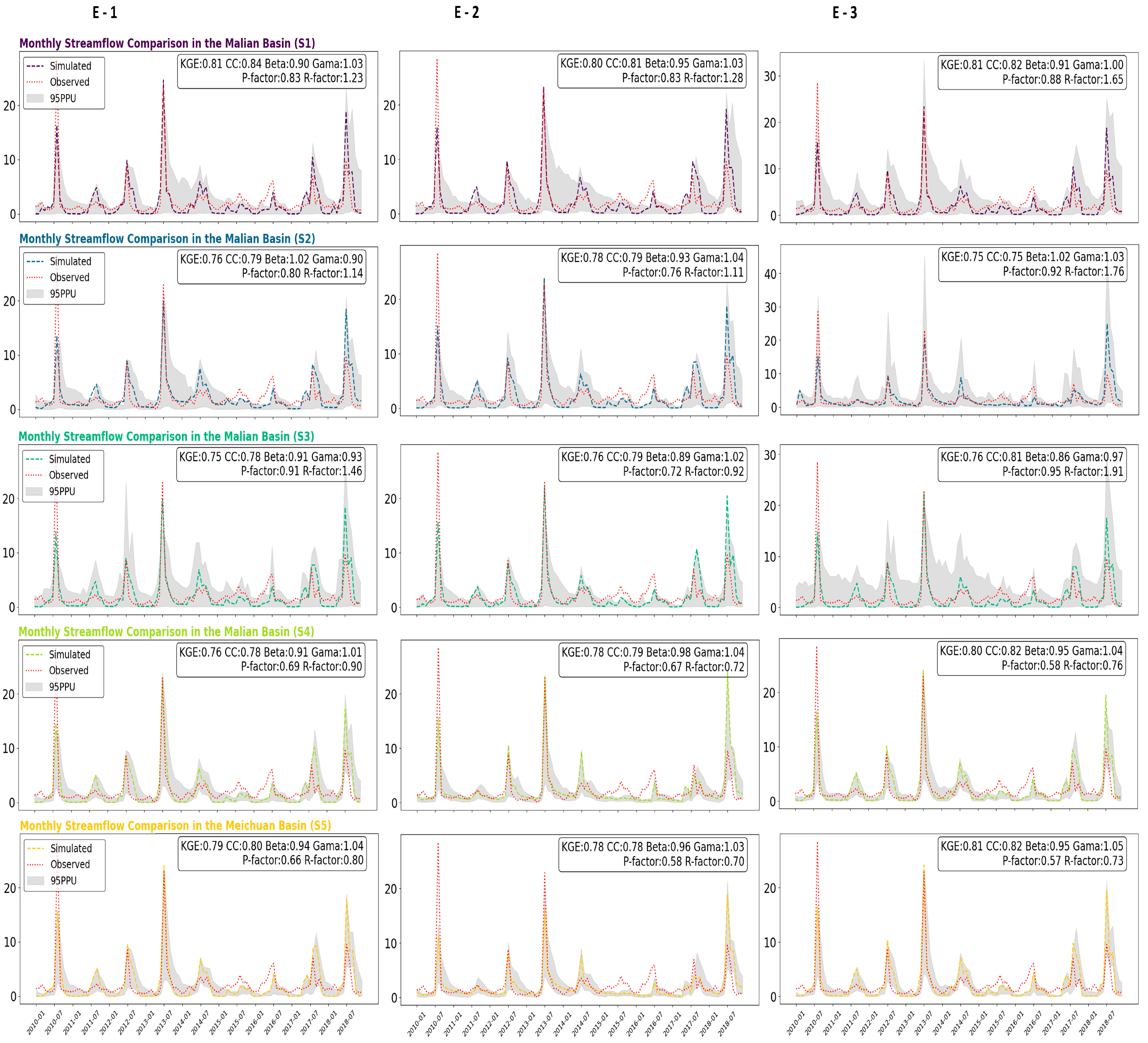
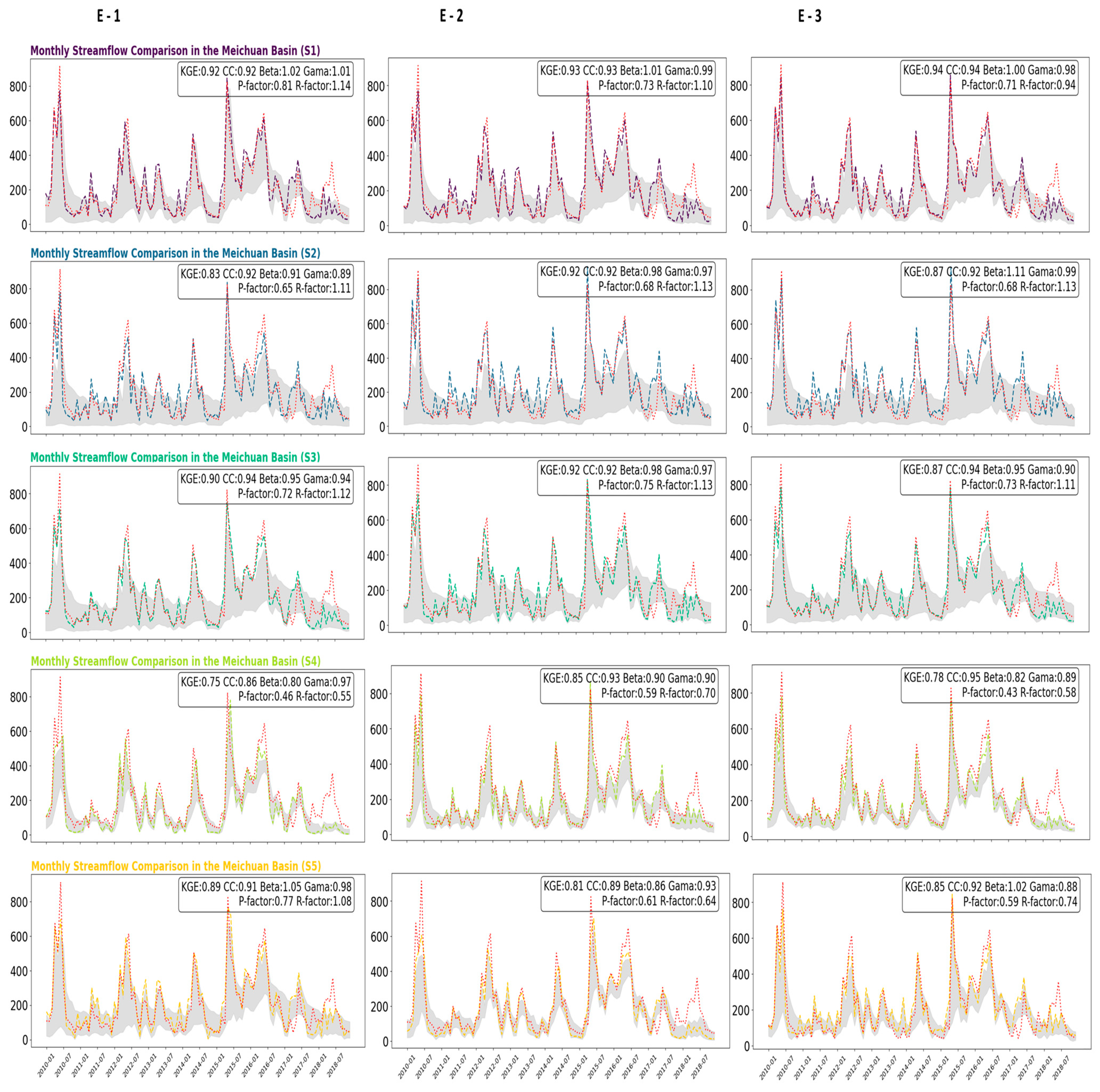
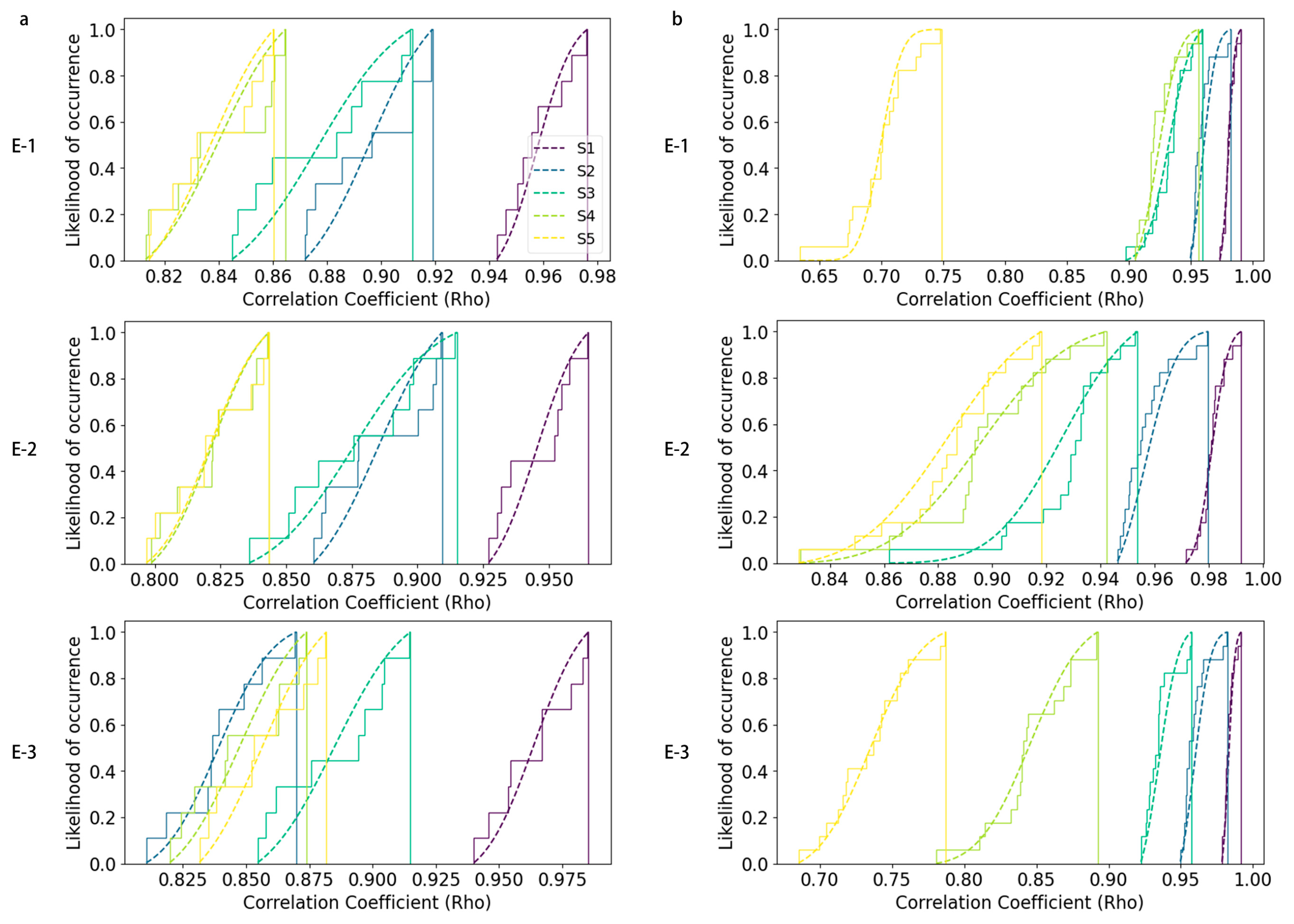
3.1. Simulated Streamflow at Gauge Stations

The time series analysis of streamflow derived from the best solutions across the five schemes at measurement stations from two watersheds (Figure 6 and Figure 7,

Table 3. Comparison of KGE values for different schemes (S1, S2, S3, S4, S5) across multiple experiments (E-1, E-2, E-3) in the Malian Basin.

	Experiment	E-1	E-2	E-3
Scheme
S1		0.81	0.80	0.80
S2		0.76	0.78	0.75
S3		0.75	0.76	0.76
S4		0.76	0.78	0.80
S5		0.79	0.78	0.81

and

Table 4. Comparison of KGE values for different schemes (S1, S2, S3, S4, S5) across multiple experiments (E-1, E-2, E-3) in the Meichuan Basin.

	Experiment	E-1	E-2	E-3
Scheme
S1		0.92	0.93	0.94
S2		0.83	0.92	0.87
S3		0.75	0.85	0.78
S4		0.76	0.78	0.80
S5		0.89	0.81	0.85

) shows clear seasonal and interannual patterns. Within these schemes, iterative optimal solutions for streamflow simulation at the Jiaqiao station in the Malian Basin (Figure 1) indicate that S1 outperforms S2 and S3, particularly in achieving a better performance (KGE > 0.8) in three trials. S1 also exhibits a higher correlation coefficient (CC), suggesting a stronger linear correlation between the simulated and observed streamflows. S1 demonstrates a greater accuracy in the beta and gamma metrics, converging to values close to 1. S4 and S5, which utilize a joint calibration approach, display comparable performance levels in streamflow simulation to S1. This is due to the challenges faced by the SWAT model in simulating streamflow in arid regions, where differences in streamflow among candidate solutions are more pronounced than in ET. As a result, the calibration process often compromises the accuracy of ET simulation. Moreover, in joint calibration, all parameters are iterated simultaneously, enabling satisfactory results to be obtained within a limited number of iterations. Nevertheless, additional iterations aimed at gathering parameters typically result in a smaller width of the 95PPU, at the expense of a P factor less than 0.7, leading to more observed points falling outside the prediction interval [58]. These findings underscore the value of the proposed calibration approach, particularly in the context of arid regions, where streamflow simulation poses a greater challenge. The performance improvements observed with S1 suggest that it may be a more reliable choice for streamflow prediction in such environments.

The calibration results obtained with S1 contrast sharply with those of previous studies that incorporated remote sensing ET products into hydrological models. Unlike traditional calibration approaches, which often improve ET simulation accuracy at the expense of streamflow precision, S1 mitigates this trade-off, achieving performance levels comparable to or even surpassing those of joint calibration approaches that prioritize streamflow accuracy.

The iterative optimal solutions for streamflow simulation at the Fenkeng station in the Meichuan Basin (Figure 7) demonstrate that S1 consistently outperforms other schemes across all three experimental iterations (KGE > 0.9), accurately capturing both the timing and variability of peak streamflow volumes. In comparison, the simulation accuracy of S2, S3, S4, and S5 declined to varying degrees due to the uncertainty inherent in the ET observation data. This decline was particularly pronounced in S4 and S5, which employed joint calibration methods. Notably, in humid catchment areas—unlike arid zones—the quality of uncertain data, such as remote sensing and reanalysis ET products, requires more careful consideration when applying joint calibration methods.

Additionally, S1 not only yielded the largest P factor but also kept the R factor within a reasonable range. This suggests that S1, compared to traditional calibration strategies, not only meets precision requirements but also ensures the reliability and robustness of the model outputs. Overall, the S1 calibration strategy demonstrates a superior performance in simulating watershed streamflow across various environmental conditions, striking a balance between accuracy and stability in its predictions.

Additionally, for each experiment, the accuracy of the top ten solutions for each scheme converges to a specific value as the number of iterations increases. In the case of S1, the solutions consistently converge towards the highest accuracy in the final iterations, demonstrating its reliability and stability. This convergence pattern holds true across all three experiments in both arid and humid regions, further emphasizing the robustness of S1. In contrast, schemes such as S2 and S3 do not exhibit this clear convergence towards a higher accuracy. Instead, their solutions are more dispersed throughout the iterations, lacking a discernible trend of improvement. This suggests that the solutions generated in these schemes are less reliable and highly sensitive to the initial conditions, leading to inconsistencies across iterations.

For S4 and S5, the iteration results show significant variability, with performance depending on the environmental conditions of the watershed. The differences in performance between arid and humid regions may be due to the dominant hydrological processes in these contrasting environments, which influence the effectiveness of the calibration strategies employed by S4 and S5. Specifically, in arid regions (Figure 8(1)), both S4 and S5 show rapid convergence, reaching the Cohen’s d standard by the fourth iteration. However, in humid regions (Figure 8(2)), their performance is highly variable, and they do not consistently achieve the highest accuracy. This suggests that traditional joint parameter tuning methods may not be well-suited to incorporating uncertain ET data in humid environments.

Overall, the experimental results indicate that S1 is the most reliable and stable strategy for streamflow simulation, while the effectiveness of other schemes varies considerably based on environmental conditions and their relative calibration stability to the initial solutions.

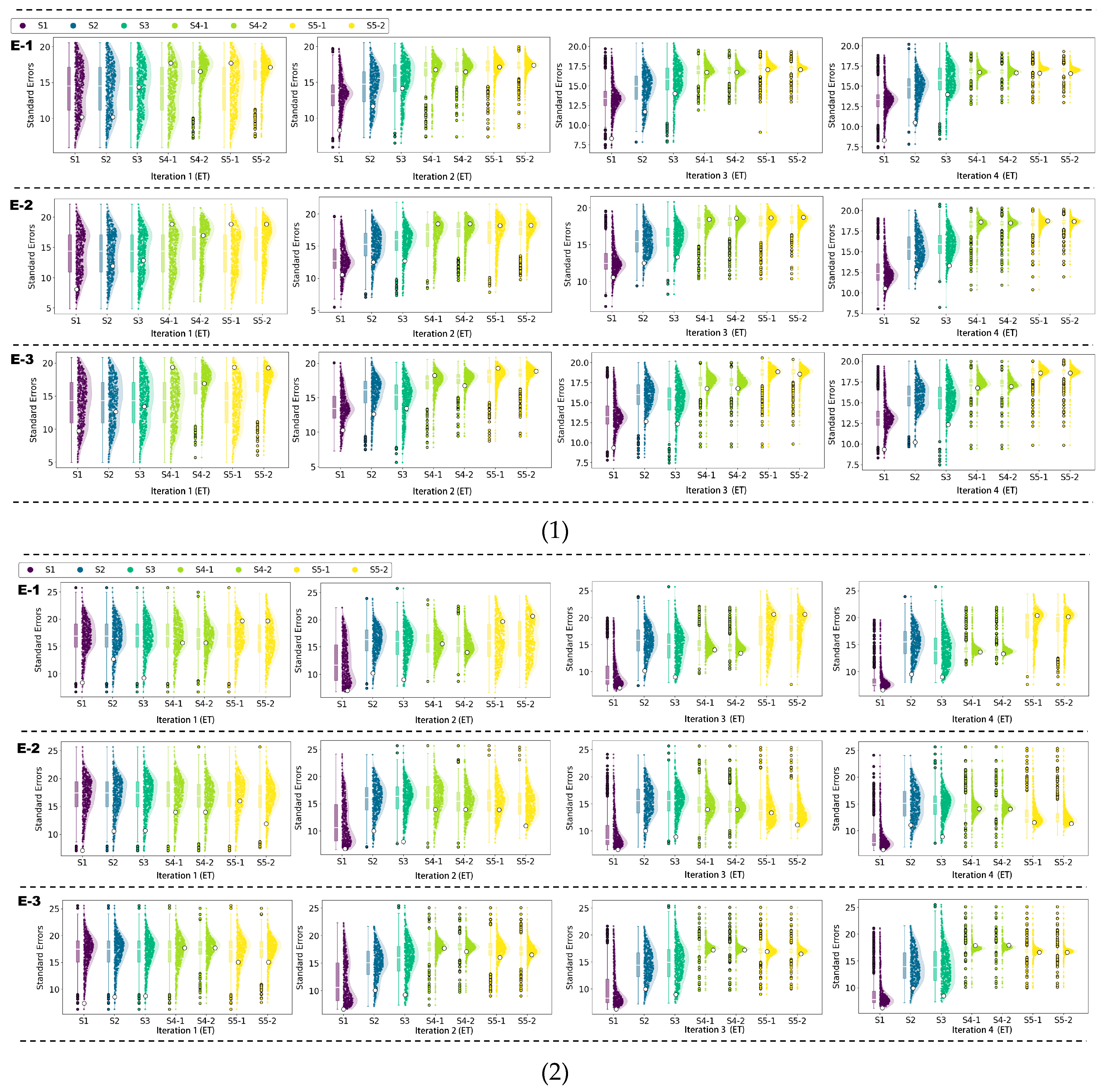
3.2. Simulated ET in Sub-Basins

Figure 9 presents the average ET simulation values across the sub-basins of the Malian Basin, an arid region. Among all the scenarios tested, S1 consistently shows stable ET values across the three experiments, demonstrating that the calibration technique is reliable and effectively simulates ET, regardless of initial conditions. In contrast, S2, S3, S4, and S5 exhibit noticeable spatial variations, with the third round of ET simulations in S2 showing significant skewness, reflecting substantial variability.

In the Meichuan Basin, Figure 10 illustrates that S1 maintains high spatial consistency in ET simulation values. However, S2 through S5 display considerable spatial variability in ET values, highlighting the impact of the selected ET products on spatial coherence within the sub-basin. Specifically, S2 tends to produce higher simulated values, while S3 generates lower values. This trend aligns with the deviations observed in the GLASS and PMLv2 products when compared to observations at the Qianyanzhou station, as shown in the Supplementary Materials, Section S2. Notably, the simulated values of S1 fall between those of S2 and S3, effectively reducing biases’ influence introduced by remote sensing ET data.

The cumulative step histograms (Figure 11) display the Rho values for the best ET indicator fit curves at the sub-basin scale within the Malian and Meichuan Basins, highlighting significant differences among the five approaches under arid and humid basin conditions. S1 consistently outperforms the other schemes, with a notably higher Rho across all experiments, regions, and percentiles. In the Malian Basin, the performance differences among S2, S3, S4, and S5 are less pronounced. However, in the Meichuan Basin, clear distinctions emerge. The results suggest that schemes using the GLASS product outperform those using PMLv2, which is consistent with the superior quality of the GLASS and PMLv2 product data, as illustrated in Supplementary Materials Figure S3.

The refined evaluation of the coefficient of determination using ETC for ET simulations reveals a clear divergence in performance among the different schemes. This analysis, which considers ET outputs from 500 candidate solutions iteratively generated within the sub-basins of both the Malian and Meichuan Basins, is graphically depicted in Figure 12. The boxplots for the two study areas clearly show that S1’s coefficient of determination is consistently higher throughout the iterative process, spanning all experiments and study areas. Additionally, stepwise calibration generally outperforms joint calibration.

Distinct contrasts emerge between S2, S3, S4, and S5 when comparing the Malian and Meichuan Basins. In the Meichuan Basin, strategies incorporating the GLASS product typically outperform those using PMLv2. However, in the Malian Basin, these differences are less pronounced. As shown in Figure 12(1.E-2), PMLv2 calibration achieves better results, while in Figure 12(1.E-3), the advantage shifts slightly to GLASS. This difference reflects the lack of a significant quality distinction between the GLASS and PMLv2 ET products in the Malian Basin, whereas in the Meichuan Basin, the quality of the GLASS product is notably superior to that of PMLv2.

Moreover, this variability suggests that the effectiveness of each scheme fluctuates with each iteration and between basins, highlighting the importance of adaptive calibration strategies and the reliability of data, which can respond to the unique hydrological processes of each sub-basin.

4. Discussion

4.1. Are the ETC-Estimated Metrics More Effective than Traditional Evaluation Methods?

The box plots in Figure 13 display the standard error (Stderr) for evapotranspiration (ET) simulations across the five calibration schemes during the three repeated experiments. Scheme S1, which utilizes the ETC-estimated determination coefficient index, consistently achieves exceptionally low standard errors. It also shows the lowest median standard error among 500 solutions in each iteration. In contrast, the remaining schemes (S2, S3, S4, S5) rely on the traditional Kling–Gupta Efficiency (KGE) index.

These findings undeniably highlight the exemplary performance of S1 in comparison to the other four scenarios. These five schemes use different metrics and calibration methodologies to determine their respective optimal solutions. Notably, the verification of these optimal solutions for each scheme uses the same measurement standard (Stderr), which differs from the measurement standards employed during the calibration process. This illustrates that S1’s superior performance does not depend on the evaluative metric standard used, but rather stems from the inherent characteristics of the ETC-based metric standard used during S1’s calibration.

ETC estimates both the Rho and Stderr of the simulated ET relative to the actual values, which makes it independent of the Stderr of the remote sensing ET products. This insensitivity to biases minimizes their impact on S1. In contrast, as evidenced in studies by [1,12,31], Scheme S2 to S5 treat the values of remote sensing ET products as ground truth, profoundly influencing the accuracy of simulated ET according to the inherent Stderr and bias of the ET products themselves. As demonstrated in Supplementary Material Section S2, products like GLASS and PMLv2 exhibit notable standard errors and biases, especially in the Meichuan watershed, where the PMLv2 product significantly underestimates ET compared to observations at the Qianyanzhou station.

Thus, compared to traditional calibration strategies, S1’s distinction lies in its ability to maintain a high correlation with true values (as shown in Figure 10), while significantly reducing the standard error of simulation under conditions where the remote sensing ET carries a significant bias. By effectively minimizing the impact of this bias, S1 consistently outperforms the other four schemes.

4.2. Is the Optimization of Parameters Across Processes with the Learning Rate More Effective than the Traditional Method?

The proposed approach aims to calibrate multiple variables by adjusting a set of parameter values, ensuring that simulations of all processes align with their corresponding observed values. However, a challenge arises when fine-tuning a parameter within a specific process to optimize performance, which might negatively affect other processes. To maintain balanced parameter assignments across all processes, significant emphasis is placed on the parameter–process relations, as detailed in Section 2.3. As shown in

Table 5. The parameter–process relations and learning rates in the experiment (illustrated with selected parameters from the four categories).

	Parameters	CH_K2	EPCO	ALPHA_BF	SOL_AWC
Processes (Variable)
Evapotranspiration (ET)		Unrelated [0]	Strong [2]	Moderate [1.5]	Weak [0.5]
Channel routing (Streamflow)		Strong [2]	Unrelated [0]	Unrelated [0]	Weak [0.5]

, parameters closely associated with the targeted process are expected to converge rapidly, resulting in a narrow parameter solution cantered around the optimal solution. In contrast, parameters less directly related to the process tend to narrow their solution more gradually.

When analyzing the outputs associated with Supplementary Materials Table S4, notable performances were observed in both evapotranspiration (ET) and channel routing (streamflow) processes. Iterative analysis of ranking scores from 500 candidate solutions revealed a gradual decrease in standard error. Scatter plots in Figure 12 illustrate a convergence of scores for all solutions toward a higher value. Parameter updates in Supplementary Materials Table S4 follow the expected pattern, with standard errors for parameters decreasing across iterations until reaching a small value. This underscores the effectiveness of the proposed learning rate in controlling parameter evolution, taking into account the established parameter–process relationships on a directed graph.

Additionally, by leveraging learning rates, the parameters in S1 are closely linked with their corresponding hydrological processes and align with the physical meanings of these parameters. Therefore, the model not only solves equifinality issues [59] but also validates [25] perspective that solutions generating similar outputs may be associated with uncertainty within the parameter set. In other words, even if the best parameter set deviates from the physical characteristics of the basin, it can still produce satisfying evaluation results, meaning there is no convergence of the final parameters [25].

As shown in Figure 14, under the PSO framework based on the learning rate, parameters that mainly affect a single process (such as CH_K2, EPCO, and ALPHA_BF) usually converge around the optimal solution of their related process parameters and are not affected by other processes [43]. For instance, in Figure 14(1), during the ET calibration in the Meichuan Basin, the optimal solution for the CH_K2 parameter exceeds 400 mm/h. However, since CH_K2 primarily impacts the channel routing (streamflow) process, it converges towards the peak output of the streamflow function, approximately 150 mm/h. Given that the Meichuan Basin is dominated by gravel mixed sand, excessively high channel hydraulics are undesirable [60]. Conversely, in the Malian Basin, with sand as the main type, channel hydraulics tend to have higher values (see Supplementary Materials Section S5) [43,60]. Similarly, in Figure 14(2,3), EPCO and ALPHA_BF also have a close connection with their corresponding hydrological processes. Even if the optimal solutions of evapotranspiration and the channel routing process correspond to similar parameter values, they remain unaffected by unrelated processes, effectively avoiding interference from unrelated hydrological processes.

Uniquely, the optimal solution of the SOL_AWC parameter, which affects two processes, often lies near the middle of the range (Figure 14(4)), consistent with the available water capacity calculated from soil moisture characteristics [43,61]. This approach diverges from merely classifying parameters into specific hydrological processes, which does not ensure the accurate expression of the physical meanings of the parameters across various hydrological processes, often resulting in non-convergent parameters. The relatively large final parameter solution space is primarily due to the different optimal values that parameters typically exhibit in various hydrological processes, necessitating a balance among these optimal solutions. Thus, this compromise has somewhat alleviated the problem of parameter uncertainty and is regarded as a necessary sacrifice to maintain the physical integrity of the parameters.

Correspondingly, we believe that the parameter learning rate introduced in S1 does indeed reduce parameter uncertainty, thereby effectively promoting the synchronous improvement of simulating ET and streamflow, as seen in the performances of evapotranspiration and streamflow in Section 4.1 and Section 4.2, where S1 consistently outperforms S2–S5. This is because, in traditional implementation schemes S2–S5, the updates of parameters did not consider their specific contribution to the outputs of specific process simulations. All parameter step size adjustments are treated in the same weighted manner, which often results in the optimization of parameters closely related to streamflow being affected by adjustments of irrelevant hydrological processes, or parameters that clearly affect multiple hydrological processes being assigned to a specific process. The conclusion is consistent with previous findings: this impact may result in a skew in parameter meanings when adjusting multiple variables, increasing parameter uncertainty, often manifesting as alleviating the equifinality but at the expense of sacrificing the accuracy of streamflow prediction [25,30,62].

4.3. Limitations and Future Works

The proposed approach facilitates hydrological modeling using data containing inherent uncertainties. Nevertheless, it remains reliant on the underlying assumptions of the ETC for evaluating hydrological simulations when faced with the absence of ground truth values. To enhance the assessment of model outputs with uncertain data, it is prudent to explore more advanced methods, such as multiple collocation [63] and quadric collocation [64], in future studies.

At present, our parameter–process relations have been developed by primarily considering the relations between a process and its preceding nodes. This has been simplified into four categories (strong, moderate, weak, unrelated) to outline our conceptual framework. However, in the future, there is a potential to formulate a function that quantifies the degree of relevance of a parameter linked to nodes distant along the back-propagation pathway to the node undergoing calibration.

Our proposed method has been tested in an arid and semi-arid basin and a humid basin. Hydrological modeling in arid regions can be challenging [54], and the results obtained from our study demonstrate its good performance in two different climate areas, indicating a certain degree of versatility. However, to enhance the robustness of this approach and to verify its universal applicability, further experiments are necessary in a broader range of regions. This need is particularly important because remote sensing data with inherent uncertainties have been becoming ubiquitous.

5. Conclusions

With the goal of facilitating the application of remote sensing products with inherent uncertainties in hydrological modeling, we have developed a new adaptive process-wise fitting approach to make it possible to calibrate hydrological models even when dealing with uncertain data. To validate its effectiveness, this approach was implemented in one humid basin and one arid basin, employing the SWAT hydrological model and remotely sensed ET products (GLASS and PMLv2). Our results illustrated the good performance of the proposed approach in hydrological modeling.

Our study demonstrated the improved performance in both ET and streamflow simulation by leveraging the advantages of utilizing remote sensing ET products to build hydrological models at the sub-basin scale. This is in contrast to previous findings of improving ET simulation at the cost of an acceptable reduction in streamflow simulation accuracy. On the contrary, our analysis of the iterative process in the experiment confirmed that the calibration strategy developed in this study, through the optimization of parameters across processes with a learning rate and the application of a model classification evaluation method considering input uncertainty, made significant contributions to reducing model parameter and input uncertainty. It facilitated parameter convergence and enhanced model accuracy, resulting in it consistently generating high-scoring solutions throughout the evolutionary steps of the model.

In conclusion, our adaptive process-wise fitting algorithm offers promising potential for integrating datasets with unknown errors into hydrological modeling. It signifies a step forward in the field of hydrology by offering a new method to handle uncertain data. It offers a new approach to hydrological process modeling in regions where ground observation stations are lacking.

References

1. Zhang, L.; Zhao, Y.; Ma, Q.; Wang, P.; Ge, Y.; Yu, W. A parallel computing-based and spatially stepwise strategy for constraining a semi-distributed hydrological model with streamflow observations and satellite-based evapotranspiration. J. Hydrol. 2021, 599, 126359. [Google Scholar] [CrossRef]
2. Shen, H.; Tolson, B.A.; Mai, J. Time to Update the Split-Sample Approach in Hydrological Model Calibration. Water Resour. Res. 2022, 58, e2021WR031523. [Google Scholar] [CrossRef]
3. Becker, R.; Koppa, A.; Schulz, S.; Usman, M.; aus der Beek, T.; Schüth, C. Spatially distributed model calibration of a highly managed hydrological system using remote sensing-derived ET data. J. Hydrol. 2019, 577, 123944. [Google Scholar] [CrossRef]
4. Hasan, H.M.; Hosseini-Moghari, S.-M.; Döll, P.; Güntner, A. Multi-variable Pareto optimal calibration of the global hydrological model WaterGAP for 1500 major drainage basins around the globe. In Proceedings of the Copernicus Meetings, Vienna, Austria, 24–28 April 2023. [Google Scholar]
5. Chlumsky, R.; Mai, J.; Craig, J.R.; Tolson, B.A. Simultaneous calibration of hydrologic model structure and parameters using a blended model. Water Resour. Res. 2021, 57, e2020WR029229. [Google Scholar] [CrossRef]
6. Ougahi, J.H.; Rowan, J.S. Combining Hydrological Models and Remote Sensing to Characterize Snowpack Dynamics in High Mountains. Remote Sens. 2024, 16, 264. [Google Scholar] [CrossRef]
7. Lan, T.; Lin, K.; Xu, C.-Y.; Tan, X.; Chen, X. Dynamics of hydrological-model parameters: Mechanisms, problems and solutions. Hydrol. Earth Syst. Sci. 2020, 24, 1347–1366. [Google Scholar] [CrossRef]
8. Tian, Y.; Zhao, Y.; Li, J.; Xu, H.; Zhang, C.; Deng, L.; Wang, Y.; Peng, M. Improving CMIP6 atmospheric river precipitation estimation by cycle-consistent generative adversarial networks. J. Geophys. Res. Atmos. 2024, 129, e2023JD040698. [Google Scholar] [CrossRef]
9. Li, Z.; He, M.-Y.; Li, B.; Wen, X.; Zhou, J.; Cheng, Y.; Zhang, N.; Deng, L. Multi-isotopic composition (Li and B isotopes) and hydrochemistry characterization of the Lakko Co Li-rich salt lake in Tibet, China: Origin and hydrological processes. J. Hydrol. 2024, 630, 130714. [Google Scholar] [CrossRef]
10. Mao, H.; Wang, C.; He, Y.; Song, X.; Ma, R.; Li, R.; Duan, Z. Advancing SWAT Model Calibration: A U-NSGA-III-Based Framework for Multi-Objective Optimization. Water 2024, 16, 3030. [Google Scholar] [CrossRef]
11. Rajib, A.; Evenson, G.R.; Golden, H.E.; Lane, C.R. Hydrologic model predictability improves with spatially explicit calibration using remotely sensed evapotranspiration and biophysical parameters. J. Hydrol. 2018, 567, 668–683. [Google Scholar] [CrossRef]
12. Wambura, F.J.; Dietrich, O.; Lischeid, G. Improving a distributed hydrological model using evapotranspiration-related boundary conditions as additional constraints in a data-scarce river basin. Hydrol. Process. 2018, 32, 759–775. [Google Scholar] [CrossRef]
13. Ningthoujam, V.; Romeji, N. SWAT Model Calibration and Validation with Remotely Sensed Evapotranspiration data in Maklang-Tuyungbi-Taret lok Ungauged Basin in Manipur, India. Iran. J. Sci. Technol. Trans. Civ. Eng. 2024, 1–17. [Google Scholar] [CrossRef]
14. Herman, M.R.; Nejadhashemi, A.P.; Abouali, M.; Hernandez-Suarez, J.S.; Daneshvar, F.; Zhang, Z.; Anderson, M.C.; Sadeghi, A.M.; Hain, C.R.; Sharifi, A. Evaluating the role of evapotranspiration remote sensing data in improving hydrological modeling predictability. J. Hydrol. 2018, 556, 39–49. [Google Scholar] [CrossRef]
15. Rajib, M.A.; Merwade, V.; Yu, Z. Multi-objective calibration of a hydrologic model using spatially distributed remotely sensed/in-situ soil moisture. J. Hydrol. 2016, 536, 192–207. [Google Scholar] [CrossRef]
16. Zejun, L.; Pan, L.; Maoyuan, F.; Xueqing, C.; Ping, H.; Caijun, W.; Jingwen, Z. Evaluating the Effect of Transpiration in Hydrologic Model Simulation through Parameter Calibration. J. Hydrol. Eng. 2020, 25, 123944. [Google Scholar]
17. van Griensven, A.; Ndomba, P.; Yalew, S.; Kilonzo, F. Critical review of SWAT applications in the upper Nile basin countries. Hydrol. Earth Syst. Sci. 2012, 16, 3371–3381. [Google Scholar] [CrossRef]
18. Ochege, F.U.; Shi, H.; Li, C.; Ma, X.; Igboeli, E.E.; Luo, G. Assessing Satellite, Land Surface Model and Reanalysis Evapotranspiration Products in the Absence of In-Situ in Central Asia. Remote Sens. 2021, 13, 5148. [Google Scholar] [CrossRef]
19. Velpuri, N.M.; Senay, G.B.; Singh, R.K.; Bohms, S.; Verdin, J.P. A comprehensive evaluation of two MODIS evapotranspiration products over the conterminous United States: Using point and gridded FLUXNET and water balance ET. Remote Sens. Environ. 2013, 139, 35–49. [Google Scholar] [CrossRef]
20. McColl, K.A.; Vogelzang, J.; Konings, A.G.; Entekhabi, D.; Piles, M.; Stoffelen, A. Extended triple collocation: Estimating errors and correlation coefficients with respect to an unknown target. Geophys. Res. Lett. 2014, 41, 6229–6236. [Google Scholar] [CrossRef]
21. Chen, F.; Crow, W.T.; Bindlish, R.; Colliander, A.; Burgin, M.S.; Asanuma, J.; Aida, K. Global-scale evaluation of SMAP, SMOS and ASCAT soil moisture products using triple collocation. Remote Sens. Environ. 2018, 214, 1–13. [Google Scholar] [CrossRef]
22. Jia, Y.; Li, C.; Yang, H.; Yang, W.; Liu, Z. Assessments of three evapotranspiration products over China using extended triple collocation and water balance methods. J. Hydrol. 2022, 614, 128594. [Google Scholar] [CrossRef]
23. Khan, M.S.; Liaqat, U.W.; Baik, J.; Choi, M. Stand-alone uncertainty characterization of GLEAM, GLDAS and MOD16 evapotranspiration products using an extended triple collocation approach. Agric. For. Meteorol. 2018, 252, 256–268. [Google Scholar] [CrossRef]
24. Yin, G.; Park, J. The use of triple collocation approach to merge satellite-and model-based terrestrial water storage for flood potential analysis. J. Hydrol. 2021, 603, 127197. [Google Scholar] [CrossRef]
25. Rajib, M.A.; Merwade, V. Improving soil moisture accounting and streamflow prediction in SWAT by incorporating a modified time-dependent Curve Number method. Hydrol. Process. 2016, 30, 603–624. [Google Scholar] [CrossRef]
26. Abbas, S.A.; Bailey, R.T.; White, J.T.; Arnold, J.G.; White, M.J.; Čerkasova, N.; Gao, J. A framework for parameter estimation, sensitivity analysis, and uncertainty analysis for holistic hydrologic modeling using SWAT+. Hydrol. Earth Syst. Sci. 2024, 28, 21–48. [Google Scholar] [CrossRef]
27. Eini, M.R.; Massari, C.; Piniewski, M. Satellite-based soil moisture enhances the reliability of agro-hydrological modeling in large transboundary river basins. Sci. Total Env. 2023, 873, 162396. [Google Scholar] [CrossRef]
28. Odusanya, A.E.; Schulz, K.; Biao, E.I.; Degan, B.A.S.; Mehdi-Schulz, B. Evaluating the performance of streamflow simulated by an eco-hydrological model calibrated and validated with global land surface actual evapotranspiration from remote sensing at a catchment scale in West Africa. J. Hydrol. Reg. Stud. 2021, 37, 100893. [Google Scholar] [CrossRef]
29. Yang, Y.; Guan, K.; Peng, B.; Pan, M.; Jiang, C.; Franz, T.E. High-resolution spatially explicit land surface model calibration using field-scale satellite-based daily evapotranspiration product. J. Hydrol. 2021, 596, 125730. [Google Scholar] [CrossRef]
30. Demirel, M.C.; Koch, J.; Rakovec, O.; Kumar, R.; Mai, J.; Müller, S.; Thober, S.; Samaniego, L.; Stisen, S. Tradeoffs between temporal and spatial pattern calibration and their impacts on robustness and transferability of hydrologic model parameters to ungauged basins. Water Resour. Res. 2024, 60, e2022WR034193. [Google Scholar] [CrossRef]
31. Herman, M.R.; Hernandez-Suarez, J.S.; Nejadhashemi, A.P.; Kropp, I.; Sadeghi, A.M. Evaluation of Multi- and Many-Objective Optimization Techniques to Improve the Performance of a Hydrologic Model Using Evapotranspiration Remote-Sensing Data. J. Hydrol. Eng. 2020, 25, 04020006. [Google Scholar] [CrossRef]
32. Gan, Y.; Liang, X.Z.; Duan, Q.; Choi, H.I.; Dai, Y.; Wu, H. Stepwise sensitivity analysis from qualitative to quantitative: Application to the terrestrial hydrological modeling of a Conjunctive Surface-Subsurface Process (CSSP) land surface model. J. Adv. Model. Earth Syst. 2015, 7, 648–669. [Google Scholar] [CrossRef]
33. Abbaspour, K.C. SWAT calibration and uncertainty programs. A User Man. 2015, 103, 17–66. [Google Scholar]
34. Singh, A.; Jha, S.K. Identification of sensitive parameters in daily and monthly hydrological simulations in small to large catchments in Central India. J. Hydrol. 2021, 601, 126632. [Google Scholar] [CrossRef]
35. Niraula, R.; Meixner, T.; Norman, L.M. Determining the importance of model calibration for forecasting absolute/relative changes in streamflow from LULC and climate changes. J. Hydrol. 2015, 522, 439–451. [Google Scholar] [CrossRef]
36. Dangol, S.; Zhang, X.; Liang, X.-Z.; Anderson, M.; Crow, W.; Lee, S.; Moglen, G.E.; McCarty, G.W. Multivariate calibration of the SWAT model using remotely sensed datasets. Remote Sens. 2023, 15, 2417. [Google Scholar] [CrossRef]
37. Li, Z.; Liu, W.-z.; Zhang, X.-c.; Zheng, F.-l. Impacts of land use change and climate variability on hydrology in an agricultural catchment on the Loess Plateau of China. J. Hydrol. 2009, 377, 35–42. [Google Scholar] [CrossRef]
38. Zhao, F.; Wu, Y.; Qiu, L.; Sun, Y.; Sun, L.; Li, Q.; Niu, J.; Wang, G. Parameter Uncertainty Analysis of the SWAT Model in a Mountain-Loess Transitional Watershed on the Chinese Loess Plateau. Water 2018, 10, 690. [Google Scholar] [CrossRef]
39. Zhang, L.; Podlasly, C.; Feger, K.-H.; Wang, Y.; Schwärzel, K. Different land management measures and climate change impacts on the runoff—A simple empirical method derived in a mesoscale catchment on the Loess Plateau. J. Arid Environ. 2015, 120, 42–50. [Google Scholar] [CrossRef]
40. Huo, J.; Liu, L. Evaluation method of multiobjective functions’ combination and its application in hydrological model evaluation. Comput. Intell. Neurosci. 2020, 2020, 8594727. [Google Scholar] [CrossRef]
41. Liu, Y.; Hou, G.; Huang, F.; Qin, H.; Wang, B.; Yi, L. Directed graph deep neural network for multi-step daily streamflow forecasting. J. Hydrol. 2022, 607, 127515. [Google Scholar] [CrossRef]
42. Fenicia, F.; Savenije, H.H.; Matgen, P.; Pfister, L. Understanding catchment behavior through stepwise model concept improvement. Water Resour. Res. 2008, 44, 1–13. [Google Scholar] [CrossRef]
43. Arnold, J.G.; Moriasi, D.N.; Gassman, P.W.; Abbaspour, K.C.; White, M.J.; Srinivasan, R.; Santhi, C.; Harmel, R.D.; van Griensven, A.; Van Liew, M.W.; et al. SWAT: Model Use, Calibration, and Validation. Trans. ASABE 2012, 55, 1491–1508. [Google Scholar] [CrossRef]
44. Arsenault, R.; Brissette, F.P. Continuous streamflow prediction in ungauged basins: The effects of equifinality and parameter set selection on uncertainty in regionalization approaches. Water Resour. Res. 2014, 50, 6135–6153. [Google Scholar] [CrossRef]
45. Saltelli, A. Sensitivity analysis for importance assessment. Risk Anal. 2002, 22, 579–590. [Google Scholar] [CrossRef]
46. Gupta, H.V.; Kling, H.; Yilmaz, K.K.; Martinez, G.F. Decomposition of the mean squared error and NSE performance criteria: Implications for improving hydrological modelling. J. Hydrol. 2009, 377, 80–91. [Google Scholar] [CrossRef]
47. Abbaspour, K.C.; Yang, J.; Maximov, I.; Siber, R.; Bogner, K.; Mieleitner, J.; Zobrist, J.; Srinivasan, R. Modelling hydrology and water quality in the pre-alpine/alpine Thur watershed using SWAT. J. Hydrol. 2007, 333, 413–430. [Google Scholar] [CrossRef]
48. Bonyadi, M.R.; Michalewicz, Z. Particle swarm optimization for single objective continuous space problems: A review. Evol. Comput. 2017, 25, 1–54. [Google Scholar] [CrossRef]
49. Eberhart, R.; Kennedy, J. Particle swarm optimization. In Proceedings of the IEEE International Conference on Neural Networks, Perth, WA, Australia, 27 November–1 December 1995; pp. 1942–1948. [Google Scholar]
50. MCKAY, M. A Comparison of Three Methods for Selecting Values of Input Variables in the Analysis of Output from a Computer Code. Technometrics 1979, 21, 239–245. [Google Scholar] [CrossRef]
51. Sobol, I.M. Uniformly distributed sequences with an additional uniform property. USSR Comput. Math. Math. Phys. 1976, 16, 236–242. [Google Scholar] [CrossRef]
52. Mai, J. Ten strategies towards successful calibration of environmental models. J. Hydrol. 2023, 620, 129414. [Google Scholar] [CrossRef]
53. Fritz, C.O.; Morris, P.E.; Richler, J.J. Effect size estimates: Current use, calculations, and interpretation. J. Exp. Psychol. Gen. 2012, 141, 2. [Google Scholar] [CrossRef] [PubMed]
54. Jiang, C.; Parteli, E.J.; Xia, Q.; Yin, X.; Shao, Y. A regional hydrological model for arid and semi-arid river basins with consideration of irrigation. Environ. Model. Softw. 2022, 157, 105531. [Google Scholar] [CrossRef]
55. Ma, T.; Duan, Z.; Li, R.; Song, X. Enhancing SWAT with remotely sensed LAI for improved modelling of ecohydrological process in subtropics. J. Hydrol. 2019, 570, 802–815. [Google Scholar] [CrossRef]
56. Robert, W.M.; Gene, Y.; Claire, B.; Margaret, W.G.; Zhiming, Q.; Devendra, M.A.; Prem, B.P.; James, V.B.; Timothy, R.G. Parameterization Guidelines and Considerations for Hydrologic Models. Trans. ASABE 2015, 58, 1681–1703. [Google Scholar] [CrossRef]
57. Vaezi, A.R. Modeling Runoff from Semi-Arid Agricultural Lands in Northwest Iran. Pedosphere 2014, 24, 595–604. [Google Scholar] [CrossRef]
58. Yang, J.; Reichert, P.; Abbaspour, K.C.; Xia, J.; Yang, H. Comparing uncertainty analysis techniques for a SWAT application to the Chaohe Basin in China. J. Hydrol. 2008, 358, 1–23. [Google Scholar] [CrossRef]
59. Beven, K. Prophecy, reality and uncertainty in distributed hydrological modelling. Adv. Water Resour. 1993, 16, 41–51. [Google Scholar] [CrossRef]
60. Larose, M.; Heathman, G.; Norton, L.; Engel, B. Hydrologic and atrazine simulation of the Cedar Creek watershed using the SWAT model. J. Environ. Qual. 2007, 36, 521–531. [Google Scholar] [CrossRef]
61. Saxton, K.E.; Rawls, W.J. Soil water characteristic estimates by texture and organic matter for hydrologic solutions. Soil Sci. Soc. Am. J. 2006, 70, 1569–1578. [Google Scholar] [CrossRef]
62. Foulon, É.; Rousseau, A.N. Equifinality and automatic calibration: What is the impact of hypothesizing an optimal parameter set on modelled hydrological processes? Can. Water Resour. J. Rev. Can. Des Ressour. Hydr. 2018, 43, 47–67. [Google Scholar] [CrossRef]
63. Pan, M.; Fisher, C.K.; Chaney, N.W.; Zhan, W.; Crow, W.T.; Aires, F.; Entekhabi, D.; Wood, E.F. Triple collocation: Beyond three estimates and separation of structural/non-structural errors. Remote Sens. Environ. 2015, 171, 299–310. [Google Scholar] [CrossRef]
64. Ling, L.; Trümmer, M.R. Multiquadric collocation method with integralformulation for boundary layer problems. Comput. Math. Appl. 2004, 48, 927–941. [Google Scholar] [CrossRef]
65. He, Y.; Wang, C.; Hu, J.; Mao, H.; Duan, Z.; Qu, C.; Li, R.; Wang, M.; Song, X. Discovering Optimal Triplets for Assessing the Uncertainties of Satellite-Derived Evapotranspiration Products. Remote Sens. 2023, 15, 3215. [Google Scholar] [CrossRef]
66. Yilmaz, M.T.; Crow, W.T. Evaluation of assumptions in soil moisture triple collocation analysis. J. Hydrometeorol. 2014, 15, 1293–1302. [Google Scholar] [CrossRef]
67. Shi, C.; Xie, Z.; Qian, H.; Liang, M.; Yang, X. China land soil moisture EnKF data assimilation based on satellite remote sensing data. Sci. China Earth Sci. 2011, 54, 1430–1440. [Google Scholar] [CrossRef]
68. Meng, X.; Wang, H. Significance of the China meteorological assimilation driving datasets for the SWAT model (CMADS) of East Asia. Water 2017, 9, 765. [Google Scholar] [CrossRef]
69. Tachikawa, T.; Hato, M.; Kaku, M.; Iwasaki, A. Characteristics of ASTER GDEM version 2. In Proceedings of the 2011 IEEE International Geoscience and Remote Sensing Symposium, Vancouver, BC, Canada, 24–29 July 2011; pp. 3657–3660. [Google Scholar]
70. Abrams, M.; Crippen, R.; Fujisada, H. ASTER global digital elevation model (GDEM) and ASTER global water body dataset (ASTWBD). Remote Sens. 2020, 12, 1156. [Google Scholar] [CrossRef]
71. Zanaga, D.; Van De Kerchove, R.; Daems, D.; De Keersmaecker, W.; Brockmann, C.; Kirches, G.; Wevers, J.; Cartus, O.; Santoro, M.; Fritz, S. ESA WorldCover 10 m 2021 v200. 2022. Available online: https://worldcover2021.esa.int/download (accessed on 21 April 2023).
72. Gong, P.; Liu, H.; Zhang, M.; Li, C.; Wang, J.; Huang, H.; Clinton, N.; Ji, L.; Li, W.; Bai, Y. Stable classification with limited sample: Transferring a 30-m resolution sample set collected in 2015 to mapping 10-m resolution global land cover in 2017. Science Bulletin 2019, 64, 370–373. [Google Scholar] [CrossRef]
73. Running, S.; Mu, Q.; Zhao, M. Mod16a2 modis/terra net evapotranspiration 8-day l4 global 500m sin grid v006. NASA EOSDIS Land Processes DAAC 2017, 6. [Google Scholar]
74. He, S.; Zhang, Y.; Ma, N.; Tian, J.; Kong, D.; Liu, C. A daily and 500 m coupled evapotranspiration and gross primary production product across China during 2000–2020. Earth Syst. Sci. Data Discuss. 2022, 2022, 5463–5488. [Google Scholar] [CrossRef]
75. Yao, Y.; Liang, S.; Li, X.; Hong, Y.; Fisher, J.B.; Zhang, N.; Chen, J.; Cheng, J.; Zhao, S.; Zhang, X. Bayesian multimodel estimation of global terrestrial latent heat flux from eddy covariance, meteorological, and satellite observations. J. Geophys. Res. Atmos. 2014, 119, 4521–4545. [Google Scholar] [CrossRef]
76. Senay, G.B. Satellite psychrometric formulation of the Operational Simplified Surface Energy Balance (SSEBop) model for quantifying and mapping evapotranspiration. Appl. Eng. Agric. 2018, 34, 555–566. [Google Scholar] [CrossRef]
Figure 1. Study Area 1: Malian Basin, Gansu Province of China.
Water 16 03446 g001
Figure 2. Study Area 2: Meichuan Basin, Jingxi Province of China.
Water 16 03446 g002
Figure 3. Flowchart of the proposed adaptive process-wise fitting method.
Water 16 03446 g003
Figure 4. Representation of hydrological model (i.e., SWAT) using a directed graph, where each node symbolizes a physical process with a specific parameter set, simultaneously accepting input variables and producing output variables.
Water 16 03446 g004
Figure 5. Deterministic framework of the adaptive process-wise fitting for solution evaluation and parameter updates through an iterative procedure with a stepwise calibration of the physical processes in a looped manner.
Water 16 03446 g005
Figure 6. Comparison of observed and simulated monthly streamflows at the Jiaqiao gauge station for five schemes across three experiments (each row represents a calibration strategy, from top to bottom as S1, S2, S3, S4, S5; each column represents three repeated experiments with different initial fixed parameters as E-1, E-2, E-3, the red line represents the observed streamflow, the purple line represents the simulated streamflow from the model using calibration strategy S1, the blue line represents the simulated streamflow from the model using calibration strategy S2, the dark green line represents the simulated streamflow from the model using calibration strategy S3, the light green line represents the simulated streamflow from the model using calibration strategy S4, and the yellow line represents the simulated streamflow from the model using calibration strategy S5).
Water 16 03446 g006
Figure 7. Comparison of observed and simulated monthly streamflows at the Fenkeng gauge station for five schemes across three experiments (each row represents a calibration strategy, from top to bottom as S1, S2, S3, S4, S5; each column represents three repeated experiments with different initial fixed parameters as E-1, E-2, E-3, the red line represents the observed streamflow, the purple line represents the simulated streamflow from the model using calibration strategy S1, the blue line represents the simulated streamflow from the model using calibration strategy S2, the dark green line represents the simulated streamflow from the model using calibration strategy S3, the light green line represents the simulated streamflow from the model using calibration strategy S4, and the yellow line represents the simulated streamflow from the model using calibration strategy S5).
Water 16 03446 g007
Figure 8. Convergence of calibration strategies in streamflow simulation. (Each column represents a different calibration strategy, ordered from left to right as S1, S2, S3, S4, S5. Within each column, three lines illustrate the calibration convergence over 4 iterations (for joint calibration, it is 8 iterations) for three separate experiments, indicated as E-1, E-2, and E-3. The lines track the convergence towards optimal solution values, indicating the effectiveness and robustness of each strategy in streamflow prediction). (1) Monthly streamflow simulated by five schemes in three repeated experiments in the Malian Basin. (2) Monthly streamflow simulated by five schemes in three repeated experiments in the Meichuan Basin.
Water 16 03446 g008
Figure 9. Spatial consistency analysis of average ET simulation in Malian Basin.
Water 16 03446 g009
Figure 10. Spatial consistency analysis of average ET simulation in Meichuan Basin.
Water 16 03446 g010
Figure 11. Cumulative plots of ETC-estimated Rho of ET simulations for two gauged regions across three schemes, with subdivision of sub-basins based on gauge stations ((a): cumulative histograms (Rho) in Malian Basin, (b): cumulative histograms (Rho) in Meichuan Basin; three separate experiments, indicated as E-1, E-2, and E-3. The purple line represents the simulated results from the model using calibration strategy S1, the blue line represents the simulated results from the model using calibration strategy S2, the dark green line represents the simulated results from the model using calibration strategy S3, the light green line represents the simulated results from the model using calibration strategy S4, and the yellow line represents the simulated results from the model using calibration strategy S5).
Water 16 03446 g011
Figure 12. Box plots of ETC-estimated coefficient of determination for ET simulations: For the measured regions of Malin and Meichuan, each round of iteration. (Experiments E-1, E-2, and E-3 represent different initial solutions, with each experiment consisting of 4 iterations (for joint calibration, it is 8 iterations). The order of the plots is from left to right, top to bottom). (1) Malian Basin. (2) Meichuan Basin.
Water 16 03446 g012aWater 16 03446 g012b
Figure 13. Box plots of Stderr for ET simulations: For the measured areas of Malin and Meichuan, each round of ET-related iterations. (Experiments E-1, E-2, and E-3 represent different initial solutions, each consisting of 4 iterations (for joint calibration, it is 8 iterations). For stepwise calibration, iterations 1, 3, 5, and 7 are included, while joint calibration includes all iterations. The order of the plots is from left to right, top to bottom. The white dots in the plots represent the optimal solutions obtained using the objective function (KGE or ETC-estimated coefficient of determination) during the iteration process). (1) Malian Basin. (2) Meichuan Basin.
Water 16 03446 g013
Figure 14. Renewed parameters converging with learning rates defined by parameter–process relations, as the ranking scores improve based on statistics from 500 candidate solutions in the evolution process. (For a schematic representation of the iteration process of all parameters across three experiments in the two study areas, see Supplementary Materials Sections S5 and S6, the red dotted lines represent the objective function values that meet the accuracy requirements). (1) CH_K2—narrowed when fitting streamflow. (CH_K2 denotes the effective hydraulic conductivity in main channel alluvium (mm/h), which is a strong parameter impacting the channel routing (streamflow) process. Therefore, iterations are only performed when calibrating the streamflow. Even though CH_K2 is involved in the calibration process for evapotranspiration (ET), the default value derived from the streamflow iteration is used). (2) EPCO—narrowed when fitting ET. (EPCO represents the plant uptake compensation factor, which is a strong parameter influencing the evapotranspiration (ET) process. Therefore, iterations are only performed during the calibration of ET. Even when EPCO is involved in the calibration process for streamflow, the default value derived from the ET iteration is used). (3) ALPHA_BF—narrowed when fitting simulated streamflow. (ALPHA_BF represents the baseflow alpha factor (1/days), which is a moderate parameter indirectly affecting the channel routing (streamflow) process by impacting the groundwater process. Therefore, iterations are only performed when calibrating the streamflow. Even though ALPHA_BF is involved in the calibration process for evapotranspiration (ET), the default value derived from the streamflow iteration is used). (4) SOL_AWC—narrowed when fitting both simulated streamflow and ETb (SOL_AWC refers to the available water capacity of the soil layer (mm H2O/mm soil). It is a weak parameter that indirectly affects both the channel routing (streamflow) and evapotranspiration (ET) processes by influencing the soil water process. Therefore, iterations are performed during the calibration of both streamflow and ET).
Water 16 03446 g014aWater 16 03446 g014bWater 16 03446 g014c