A Hybrid Approach of Air Mass Trajectory Modeling and Machine Learning for Acid Rain Estimation

Abstract

This study employed machine learning, specifically deep neural networks (DNNs) and long short-term memory (LSTM) networks, to build a model for estimating acid rain pH levels. The Yangming monitoring station in the Taipei metropolitan area was selected as the research site. Based on pollutant sources from the air mass back trajectory (AMBT) of the HY-SPLIT model, three possible source regions were identified: mainland China and the Japanese islands under the northeast monsoon system (Region C), the Philippines and Indochina Peninsula under the southwest monsoon system (Region R), and the Pacific Ocean under the western Pacific high-pressure system (Region S). Data for these regions were used to build the ANN_AMBT model. The AMBT model provided air mass origin information at different altitudes, leading to models for 50 m, 500 m, and 1000 m (ANN_AMBT_50m, ANN_AMBT_500m, and ANN_AMBT_1000m, respectively). Additionally, an ANN model based only on ground station attributes, without AMBT information (LSTM_No_AMBT), served as a benchmark. Due to the northeast monsoon, Taiwan is prone to severe acid rain events in winter, often carrying external pollutants. Results from these events showed that the LSTM_AMBT_500m model achieved the highest percentages of model improvement rate (MIR), ranging from 17.96% to 36.53% (average 27.92%), followed by the LSTM_AMBT_50m model (MIR 12.94% to 26.42%, average 21.70%), while the LSTM_AMBT_1000m model had the lowest MIR (2.64% to 12.26%, average 6.79%). These findings indicate that the LSTM_AMBT_50m and LSTM_AMBT_500m models better capture pH variation trends, reduce prediction errors, and improve accuracy in forecasting pH levels during severe acid rain events.

1. Introduction

Taiwan, located at the intersection of East Asia and the western Pacific, is subject to the long-term influence of the winter northeasterly monsoon and the summer southwesterly monsoon. This makes northern Taiwan especially susceptible to the transport of acidic pollutants, including acidic wet deposition from East Asia and mainland China. The precursor pollutants of acid rain undergo extensive chemical reactions in the atmosphere and within clouds, forming sulfuric acid and suspended particles, which then settle to the ground through dry and wet deposition processes [1,2,3]. Therefore, the study of acid rain pollution in Taiwan must account for the impacts of long-range transport of these pollutants.

The pH concentration of acidic wet deposition in the environment has a significant impact on human health and economic assets. Therefore, this study utilizes monitoring data on air quality and meteorological factors as attribute data, combined with air mass trajectory information, to fully account for factors such as seasonal atmospheric transport and pollutant source regions. The aim is to develop a model capable of accurately predicting the pH concentration of rainwater in the target area, allowing the public to be alerted to the threats posed by acid rain pollution in advance.

Atmospheric acidification, acid rain (the acidity of wet deposition), global chemical changes caused by ozone, ecological imbalance, and climate change induced by greenhouse gases are recognized as the four major environmental challenges facing humanity [4,5]. Research indicates that the formation of acid rain is influenced not only by local acidic substances but also by high-altitude pollutants, which can affect acid rain formation over distances of hundreds to thousands of kilometers through atmospheric transport [6,7]. Regional transport is thus considered a key factor in the intensification of acid rain within affected areas [8,9].

Regarding research on rainwater pH, most studies have focused on two major areas: regional sampling analysis and simulated estimation of the impact of pollutants on rainwater acidity. Sample analysis can reveal certain characteristics of acid rain in a specific region. However, since acid rain is the result of multifactorial interactions, any analysis must encompass a range of factors [10,11]. Geographic location, topography, precursor pollutants, and meteorological conditions are commonly used to predict the distribution of acid rain [12,13,14]. A comprehensive long-term study on acid deposition initiated in 1990 revealed that acid rain has become widespread across Taiwan, with the probability of occurrence exceeding 50% [2]. Urban areas, particularly Taipei in northern Taiwan, experienced higher rates, with occurrences reaching up to 85%, while suburban areas recorded fewer events. Similar studies in Northeast China also examined the spatiotemporal variations of acid rain, providing further insights into regional pollution dynamics.

Understanding airflow trajectory patterns and exploring the characteristics of acid rain under different seasonal climate patterns are crucial for investigating the pH of rainwater [15,16]. This emphasizes the significance of comprehending pollutant transport and dispersion processes to gain insights into the factors affecting acid rain characteristics. Many studies have applied the use of air mass back trajectory (AMBT), which serves the purpose of tracking the air mass origins at specific locations [17,18,19]. Using the AMBT model, the acidic aerosol sources can be classified.

As a subtropical island nation with a near-equatorial climate, Taiwan’s weather patterns are strongly influenced by warm, moist air currents and oceanic conditions. Additionally, its proximity to the mainland exposes it to continental climate influences. In their aerosol study of Keelung City, Taiwan, Chen and Chen [3] noted that most nitrogen species are associated with inorganic particles originating from mainland China, influenced by factors such as continental weathering, biomass burning, and anthropogenic combustion.

Acid rain, driven by the interaction of multiple variables and the cross-border transport of pollutants, poses challenges for accurately predicting acidic wet deposition. Early studies relied on statistical regression models; for example, Stein et al. [20] used a simple regression model to estimate annual sulfate wet deposition at monitoring sites during the 1980s, effectively assessing the impact of changes in pollutant emissions on sulfate concentrations in precipitation.

In recent years, machine learning, as part of artificial intelligence (AI) technologies, has also been applied to predict rainwater pH. For instance, Ma [21] used an artificial neural network (ANN) for acid deposition predictions, collecting data from monitoring sites across the U.S. As ANN technology has advanced, more research has been dedicated to estimating acid rain [14,15]. Zhu et al. [22] proposed an intelligent optimization algorithm to predict the pollutants responsible for acid rain, namely nitrogen dioxide and sulfur dioxide. They employed a support vector regression model combined with the Cuckoo Search and Grey Wolf Optimizer. Tao et al. [23] proposed a flexible method using multilayer perceptron (MLP) neural network analysis to estimate the in situ aerosol acidity of ambient fine particles, based on inputs of water-soluble ions and meteorological parameters.

Although AI algorithms have rapidly advanced in recent years, introducing various sophisticated methods such as the long short-term memory (LSTM) networks [24] and Transformer networks [25], significantly improving predictive accuracy, current research gaps remain in the estimation of acid rain using these advanced AI algorithms. As highlighted in the aforementioned literature review, studies in this area are still relatively scarce. Recent studies utilizing various machine learning approaches (excluding neural network-based models), such as gated recurrent units (GRUs) [26] and Transformers [27,28,29], have proven highly effective in handling time-series data. Despite their potential, however, no research to date has specifically applied these RNN-based models to acid rain forecasting.

As highlighted above, RNN-based models have not yet been utilized for acid rain prediction. While models like LSTM and GRU have been applied in other areas of environmental science, their specific application to acid rain forecasting remains unexplored. This study, therefore, pioneers the use of RNN-based models for predicting acid rain.

The primary goal of this study is to develop a model capable of accurately predicting the acidity or alkalinity of rainwater in the target area. This approach aims to provide the public with timely information about the risks associated with acid rain pollution, aligning with the need for effective early prevention strategies. Utilizing monitoring data on air quality, water quality, and meteorological factors, this study employs an ANN model to estimate rainwater pH. Considering Taiwan’s complex climate and the influence of continental monsoons, incorporating the AMBT model to classify external acidic aerosol sources offers a promising approach. A review of the current literature reveals that no ANN model has yet been integrated with the AMBT model to predict rainwater pH. By including information on air mass trajectories, this study can comprehensively account for factors such as seasonal atmospheric transport and the geographic origins of pollution sources.

To summarize, the highlights of this study are as follows:

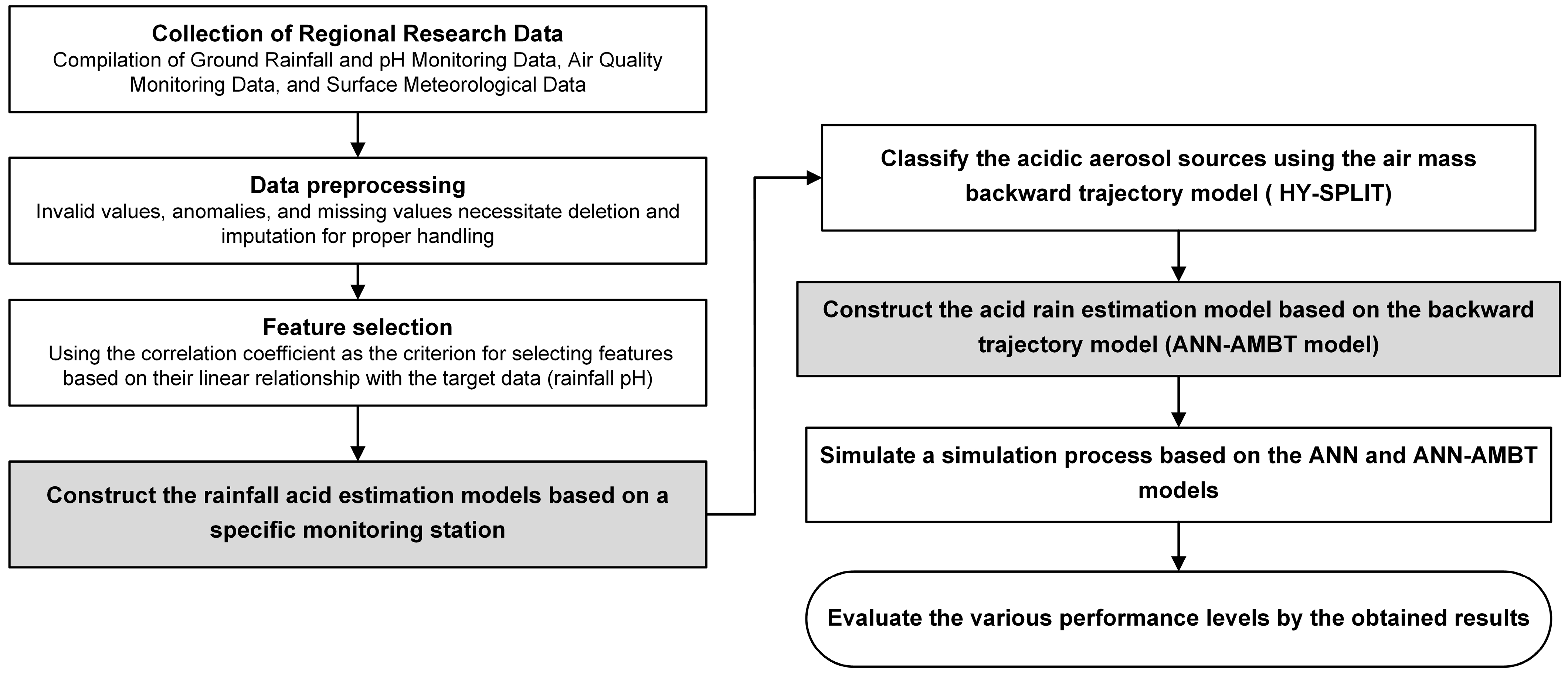
• Use of HY-SPLIT Model: This study utilizes the Hybrid Single-Particle Lagrangian Integrated Trajectory (HY-SPLIT) model, developed by the National Oceanic and Atmospheric Administration (NOAA) [30,31], to classify acidic aerosol sources through air mass back trajectory (AMBT) analysis. HY-SPLIT calculates the movement paths of air masses, providing a critical framework for identifying the origins and transport pathways of pollutants. For related studies, see [17,18,19].
• Application of AI Technologies: This research employs AI technologies, specifically machine learning, to estimate rainwater acidity. Two ANNs are utilized: deep neural networks (DNNs) with an MLP architecture and LSTM networks. The study establishes correlations between key pollutants and other relevant factors. The performance of these models in predicting rainwater acidity is then evaluated and compared. For related studies on DNN applications in acid rain forecasting, see [21,22,23]. As previously noted, no research has yet applied LSTM networks specifically to acid rain forecasting.
• Integration of AMBT Analysis and AI Technologies: To enhance prediction accuracy, this study integrates air mass trajectory data with AI models to account for the influence of atmospheric circulation on the transport of foreign chemical substances. Specifically, this approach combines machine learning techniques with meteorological data to deliver more accurate predictions of rainwater acidity. The proposed integrated model is novel and has not been documented in the existing literature. Details of this model are provided in Section 3: Methodology.

Given that the northern region of Taiwan is highly industrialized and urbanized, it is likely to exhibit a high degree of pollution dependence. Additionally, this region is influenced by its unique climatic conditions. Therefore, the northern region of Taiwan is chosen as the research area for this study.

2. Research Area and Data

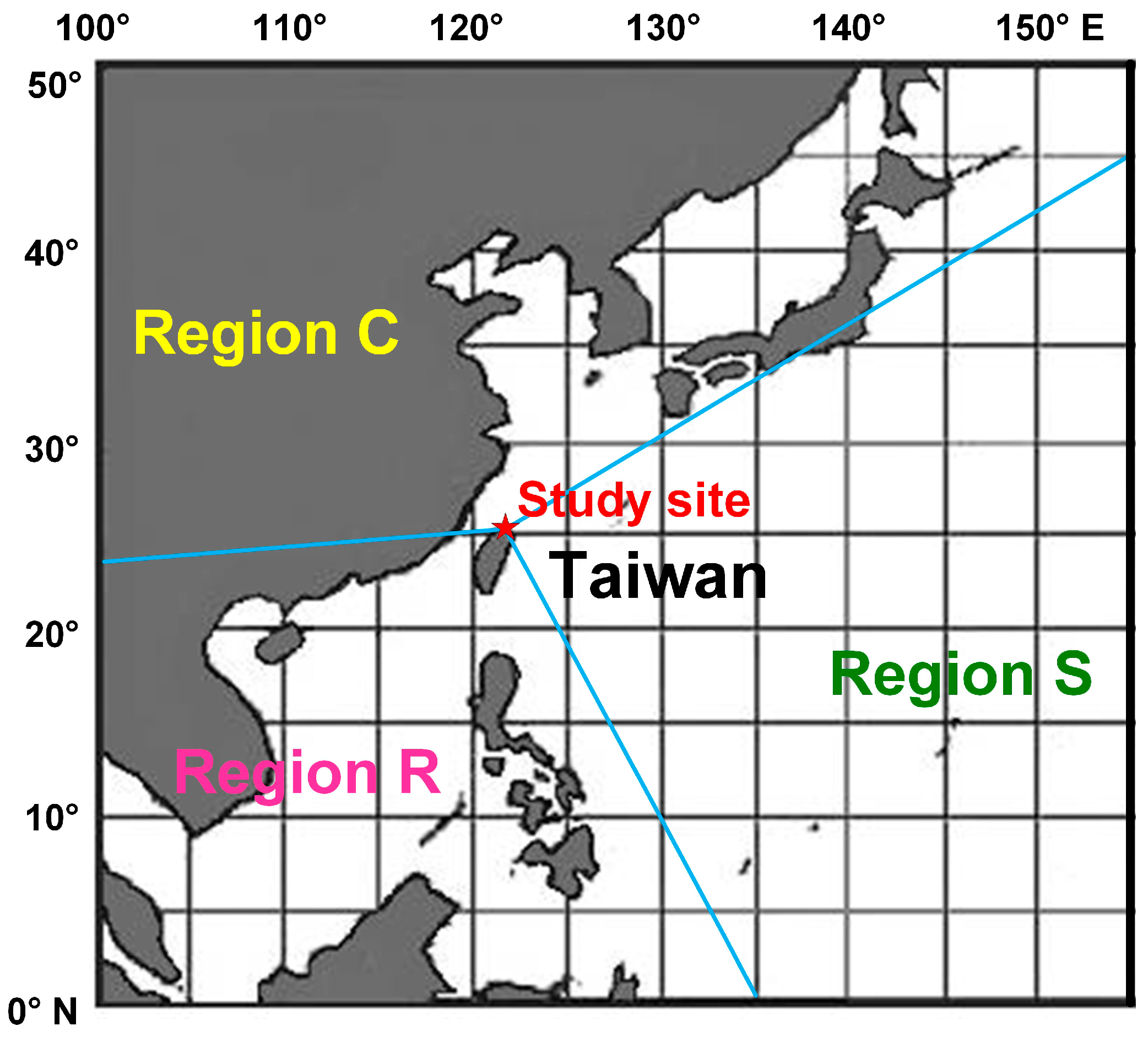
The study area is the Yangming monitoring station, located in the Greater Taipei metropolitan area in northern Taiwan (Figure 1). The Yangming monitoring station is situated within Yangmingshan National Park in Taipei City. According to Taiwan’s Ministry of Environment (MOE), the station is classified as a “park station”, distinct from general stations, traffic stations, or background stations.

The data utilized in this research were obtained from Taiwan’s MOE, comprising daily air quality monitoring values and acid rain monitoring data collected from 2008 to 2020. The dataset includes approximately 4700 daily records. A total of 13 monitoring parameters were analyzed, encompassing pollutants, acid rain, and meteorological data (as summarized in

Table 1. Parameters of pollutants, acid rain, and meteorological data at Yangming station with their statistical values.

Parameter	Unit	Range	Mean	St Dev	Parameter	Unit	Range	Mean	St Dev
PM10	μg/m3	5–83	10.84	11.12	NO2	ppb	0–7.13	1.90	1.61
PM2.5	μg/m3	0–33	6.20	7.25	RAIN_COND	μmho/cm	1.7–609.75	53.25	83.63
O3	ppb	0–78.4	40.17	11.31	PH_RAIN	pH	3.65–7.64	4.58	0.55
SO2	ppb	0–3.9	1.48	0.90	AMB_TEMP	°C	1.63–26.76	16.54	5.38
CO	ppm	0–0.45	0.16	0.09	RAIN_INT	mm/day	0.5–23.5	2.22	2.75
CO2	ppm	0–437.03	420.57	36.62	RH	%	80.77–99.59	96.57	11.22
NO	ppb	0–1.71	0.47	0.73

). These parameters include particulate matter (PM2.5), suspended particulates (PM10), ozone (O₃), sulfur dioxide (SO₂), carbon monoxide (CO), carbon dioxide (CO₂), nitrogen monoxide (NO), nitrogen dioxide (NO₂), nitrogen oxides (NO_x), rainwater conductivity (RAIN_COND), acid rain pH (PH_RAIN), atmospheric temperature (AMB_TEMP), rainfall intensity (RAIN_INT), and relative humidity (RH). The respective units for these parameters are also provided in Table 1.

Regarding data quality, some raw data included invalid values due to instrument errors, program checks, manual inspections, or equipment malfunctions. These issues also resulted in missing values, unreasonable negative values, or null entries. Among these, unreasonable negative values refer to cases where air quality monitoring parameters (e.g., PM10 and PM2.5) theoretically have a background value greater than zero. Hence, monitoring values recorded as negative or zero were deemed invalid.

To address this, data preprocessing was performed. First, raw data with poor quality control were removed, including the aforementioned invalid values. Missing data were then handled using interpolation or extrapolation methods. After preprocessing, all 13 attributes underwent further analysis to confirm their statistical validity (as shown in Table 1). The statistical summary, including minimum and maximum values, mean, and standard deviation for each attribute, indicated that the data fell within reasonable ranges.

3. Methodology

The proposed approach aims to predict the acidity of wet deposition in a specific region. This study establishes artificial neural networks, including a DNN and an LSTM neural network. These networks are trained using highly correlated features related to air quality, weather factors, and rain acidity assessment. The performance of these models is compared by inputting various climate patterns and evaluating the prediction results.

3.1. Procedure of Methodology

Figure 2 illustrates the process of developing an acid rain prediction model. It begins with examining the regional correlation between acid rain and collected climate and water parameters. Next, prediction models for acid rain are constructed using attributes from a specific monitoring station. This study employs two distinct ANN models—DNN and LSTM networks—to build these prediction models. An overview of each model is provided below.

• This study utilizes several representative DNNs to construct neural network models. DNNs are advanced models with a multi-layered architecture, representing an evolution of the MLP network. The MLP serves as the foundational structure for deep neural networks, consisting of an input layer, multiple hidden layers, and an output layer. For more details, see [32,33].
• The LSTM model features recurrently connected memory blocks, each containing self-connected memory cells and three types of gate units: input gates, output gates, and forget gates, as described by [34]. This architecture, introduced by [24], was designed to address the vanishing gradient problem prevalent in traditional recurrent neural networks. The key innovation of LSTM is its memory cell, which enables the model to maintain persistent long-term dependencies and store information across extended sequences, thereby overcoming the vanishing gradient issue [35,36]. For a comprehensive understanding, refer to the foundational work by [24].

According to Chen and Chen [3], pollution sources are classified into three potential regions (as shown in Figure 1): (1) Region C: the continent region under the northeast monsoon system, including mainland China and the Japanese archipelago; (2) Region R: the Southeast region under the southwest monsoon system, including the Philippines and the Indochina Peninsula; and (3) Region S: the sea region under the western Pacific high-pressure system.

Subsequently, this study proposes an acid rain prediction model based on ANNs that incorporates information from a backward trajectory model to estimate acidic aerosol sources (referred to as the ANN_AMBT model). Details of the modeling approach can be found in Section 4.2. In summary, the development of the acid rain pH prediction system involves integrating various models to achieve greater accuracy in estimating pH values for the study area under diverse conditions.

3.2. Role of Modularization in Each Model

In the previous section, this study modularized three models, namely (1) ANN-based acid rain estimation models, (2) AMBT analysis using the HY-SPLIT backward trajectory model, and (3) ANN_AMBT integral acid rain estimation models. The relationships among these three models are illustrated in Figure 3. The specific roles of each module in the framework are described below.

• ANN-based Acid Rain Estimation Models

These models utilize ANNs, specifically MLP and LSTM, to estimate acid rain occurrence. The MLP model captures static relationships between variables, while the LSTM model handles time-series data to account for temporal dependencies in environmental patterns.

• AMBT Analysis using HY-SPLIT Backward Trajectory Model

The HY-SPLIT model is employed to track air mass backward trajectories, that is, AMBTs. This module identifies the origins and pathways of air pollutants transported into the study region, helping to understand the external influences on acid rain formation.

• ANN_AMBT Integral Acid Rain Estimation Models

This integral model combines the strengths of ANN-based estimation models and the AMBT analysis. By integrating the predictive capabilities of the ANN models with the spatial and temporal insights provided by the HY-SPLIT trajectories, the ANN_AMBT model offers a comprehensive approach to acid rain estimation.

3.3. Criteria

This research utilizes the following evaluation metrics: root mean squared error (RMSE), mean absolute error (MAE), mean error (ME), correlation coefficient (r), mean absolute percentage error (MAPE), coefficient of variation (C.V.), and tracking signal (TS). These metrics are defined as follows:

$$\mathrm{R}\mathrm{M}\mathrm{S}\mathrm{E}=\sqrt{{\displaystyle \frac{{\sum }_{i=1}^n{\left(O_i^{Obs}-O_i^{pre}\right)}^2}{n}}}$$

(1)

$$\mathrm{M}\mathrm{A}\mathrm{E}={\displaystyle \frac{1}{n}}{\sum }_{i=1}^n\left|O_i^{Obs}-O_i^{pre}\right|$$

(2)

$$\mathrm{M}\mathrm{E}={\displaystyle \frac{1}{n}}{\sum }_{i=1}^n{O}_i^{obs}-O_i^{pre}$$

(3)

$$\mathrm{r}={\displaystyle \frac{{\sum }_{i=1}^n\left(O_i^{Obs}-{\overline{O}}^{Obs}\right)\left(O_i^{pre}-{\overline{O}}^{pre}\right)}{\sqrt{{\sum }_{i=1}^n{\left(O_i^{Obs}-{\overline{O}}^{Obs}\right)}^2}\sqrt{{\sum }_{i=1}^n{\left(O_i^{pre}-{\overline{O}}^{pre}\right)}^2}}}$$

(4)

$$\mathrm{M}\mathrm{A}\mathrm{P}\mathrm{E}={\displaystyle \frac{100\%}{n}}\stackrel{n}{\sum _{i=1}}\mid {\displaystyle \frac{O_i^{Obs}-O_i^{pre}}{{O_i}^{obs}}}\mid$$

(5)

$$\mathrm{C}.\mathrm{V}.={\displaystyle \frac{{\sigma }^{pre}}{{\overline{O}}^{pre}}}$$

(6)

$$\mathrm{T}\mathrm{S}={\displaystyle \frac{\mathrm{M}\mathrm{E}}{\mathrm{M}\mathrm{A}\mathrm{E}}}$$

(7)

where n represents the total number of data points, $O_i^{pre}$ is the ith predicted value, $O_i^{obs}$ is the ith observed value, ${\overline{O}}^{pre}$ denotes the mean of predicted values, ${\overline{O}}^{Obs}$ is the mean of observed values, and ${\sigma }^{pre}$ is the standard deviation of predicted values.

4. Modeling and Evaluation

This study begins by selecting input attributes based on their correlation with the pH of rainwater at the target monitoring station. According to Zhang et al. [37], the correlation coefficient ranges from −1 to 1. A coefficient of |r| < 0.2 indicates a very weak or no correlation, 0.2 ≤ |r| < 0.4 suggests a weak correlation, 0.4 ≤ |r| < 0.6 indicates a moderate correlation, and |r| ≥ 0.6 signifies a strong correlation. When setting the thresholds, a higher threshold results in fewer parameters being selected (e.g., if |r| is greater than 0.3, only three parameters are included), which could potentially affect the model’s quality. Ultimately, we selected parameters with |r| greater than 0.2 as input features.

Table 2. The correlation coefficients between the original monitoring data and the pH of rainwater at the target station.

Attribute	r	Attribute	r	Attribute	r
PM2.5	−0.324	CO2	−0.087	PH_RAIN	1
PM10	−0.249	NO	0.019	AMB_TEMP	0.268
O3	−0.237	NO2	−0.120	RAIN_INT	0.140
SO2	−0.227	NOx	−0.092	RH	0.038
CO	−0.316	RAIN_COND	−0.444

presents the results of the correlation analysis for various parameters, including PM2.5, PM10, O₃, SO₂, CO, RAIN_COND, PH_RAIN, and AMB_TEMP, evaluated against a threshold of r = 0.2. The analysis reveals that, apart from rainwater conductivity (RAIN_COND), the pH of rainwater is highly correlated with particulate matter concentrations (PM2.5 and PM10). This finding suggests that acidic aerosols significantly influence rainwater acidity in the region.

Features demonstrating a strong or meaningful correlation with the target variable (i.e., rainwater pH) were selected as inputs to enhance the predictive performance of the models. This approach ensures the input data captures relevant patterns for LSTM to model temporal dependencies and for DNN to identify complex nonlinear relationships effectively.

4.1. Modeling of ANN Models

The data are divided into training and validation sets using data from 2008 to 2016 (9 years) and a testing set from 2017 to 2020 (4 years) to achieve parameter verification and model evaluation objectives. Python was used as the programming language, and the Keras library, running on top of TensorFlow, was employed to develop and train the neural network models. These tools were selected for their flexibility, ease of use, and robust support for machine learning and deep learning applications. The study employs a trial-and-error approach to iteratively adjust and optimize the nonlinear mapping relationships between inputs and outputs, enhancing the model’s ability to fit the target values more accurately.

For the DNN model, several parameters require optimization, including the learning rate, the number of hidden layers, and the number of neurons per hidden layer. To optimize these networks, the study employs the Adam optimizer [38], known for its adaptive learning rates that adjust dynamically based on estimates of the first and second moments of the gradient.

• Learning Rate: This parameter is crucial during the training process as it affects the convergence speed of the model. A larger learning rate can speed up convergence but may cause oscillations (damping) and prevent reaching the function’s minimum. Conversely, a smaller learning rate results in slower convergence and may lead to getting stuck in local minima, requiring many iterations to approach the target value. The study starts with an initial learning rate of 0.1 and incrementally adjusts it by 0.1 to find the optimal learning rate.
• Number of Hidden Layers: A basic neural network model consists of three layers: input, hidden, and output. The number of hidden layers can vary, with two layers generally providing better performance compared to one layer. However, too many layers may hinder convergence and increase errors [39]. The study begins with one hidden layer and increases the number of layers until the parameter values diverge to find the optimal configuration. The number of neurons per hidden layer is initially set to 10.
• Number of Neurons per Hidden Layer: The number of neurons in the hidden layers significantly impacts the network’s computational capability. If the number of neurons is too low, the network may fail to model the relationship between inputs and outputs effectively. Conversely, too many neurons can lead to overfitting, where the model performs well on training data but poorly on new data. The study explores neuron counts in increments of 10 to find the appropriate range.

The results of the DNN parameter optimization are summarized in

Table 3. DNN model parameter tuning results.

Learning Rate	No. of Hidden Layers	No. of Neurons	RMSE	Learning Rate	No. of Hidden Layers	No. of Neurons	RMSE
0.1	1	10	0.536	0.1	1	60	0.492
0.2	1	10	0.541	0.1	1	60	0.485
0.3	1	10	0.558	0.1	2	60	0.480
0.4	1	10	0.781	0.1	3	60	0.489
0.5	1	10	0.648	0.1	4	60	0.491
0.1	1	20	0.505	0.1	5	60	0.495
0.1	1	30	0.490	0.1	6	60	0.501
0.1	1	40	0.487	0.1	7	60	0.511
0.1	1	50	0.485	0.1	8	60	0.537
0.1	1	60	0.483	0.1	9	60	0.526
0.1	1	70	0.486	0.1	10	60	0.525
0.1	1	80	0.487

. The optimal configuration identified is a learning rate of 0.1, two hidden layers, each with 60 neurons.

In addition, the parameter tuning for LSTM neural networks includes the number of hidden layers and the number of neurons per hidden layer. The parameter adjustment process follows the same method as for the DNN, where the number of hidden layers is initially set to 1 and gradually increased until the parameters diverge to find the optimal number of layers. Similarly, the number of neurons per hidden layer starts at the default value of 10 and is adjusted accordingly.

The results of the LSTM model parameter tuning are shown in

Table 4. LSTM model parameter tuning results.

Learning Rate	No. of Neurons	RMSE	Learning Rate	No. of Hidden Layers	No. of Neurons	RMSE
0.1	10	0.536	0.1	1	60	0.492
0.2	10	0.541	0.1	1	60	0.485
0.3	10	0.558	0.1	2	60	0.480
0.4	10	0.781	0.1	3	60	0.489
0.5	10	0.648	0.1	4	60	0.491
0.1	20	0.505	0.1	5	60	0.495
0.1	30	0.490	0.1	6	60	0.501
0.1	40	0.487	0.1	7	60	0.511
0.1	50	0.485	0.1	8	60	0.537
0.1	60	0.483	0.1	9	60	0.526
0.1	70	0.486	0.1	10	60	0.525
0.1	80	0.487

. The tuning initially involved adjusting the number of neurons per hidden layer, starting from 20. The model converged at this number but gradually showed signs of overfitting as more neurons were added. For the number of hidden layers, the optimal convergence was achieved with six layers, each containing 20 neurons. Therefore, the best parameter combination for the LSTM model is one hidden layer with 20 neurons per layer.

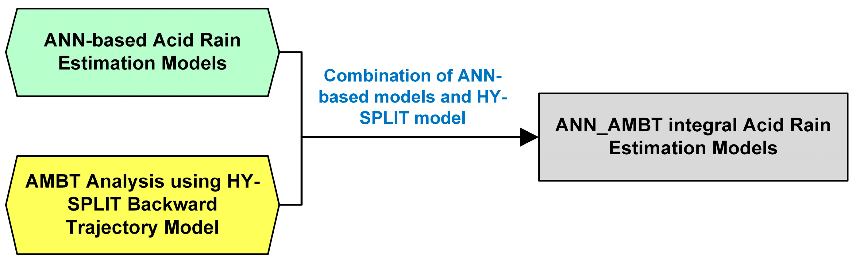
4.2. ANN_AMBT Modeling

As highlighted earlier, the ANN_AMBT modeling serves as an integral framework that merges the predictive power of ANN-based estimation models with the spatial and temporal analytical capabilities of the AMBT model. Specifically, the HY-SPLIT trajectories are employed to track the movement and origins of air masses arriving at a designated location. For this study, the AMBT model is configured to trace four-day backward trajectories of air masses, focusing on the Keelung area (near Yangming station). This setup aligns with the methodology outlined in [3], providing a robust approach to estimate the sources of air masses influencing acid rain formation.

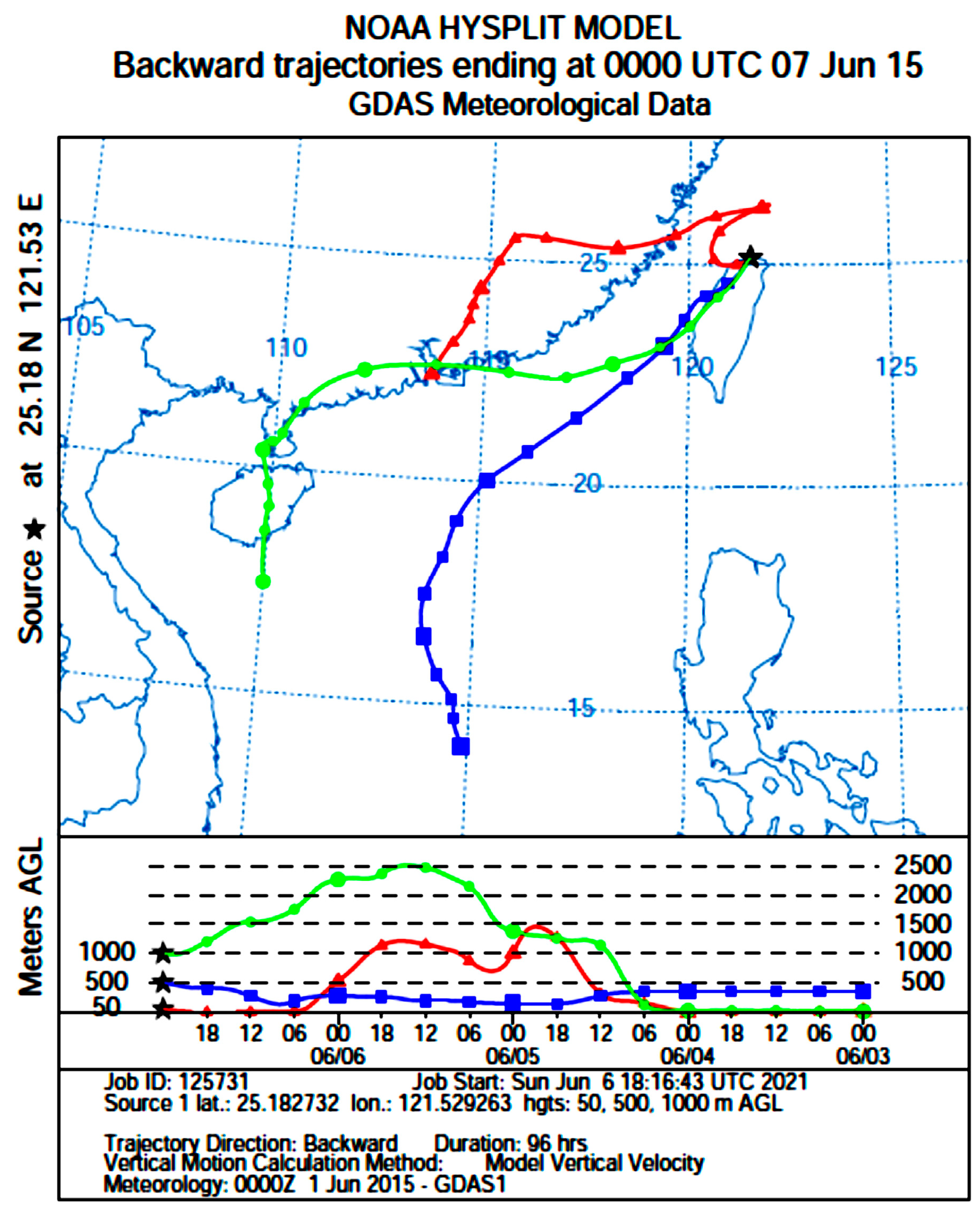
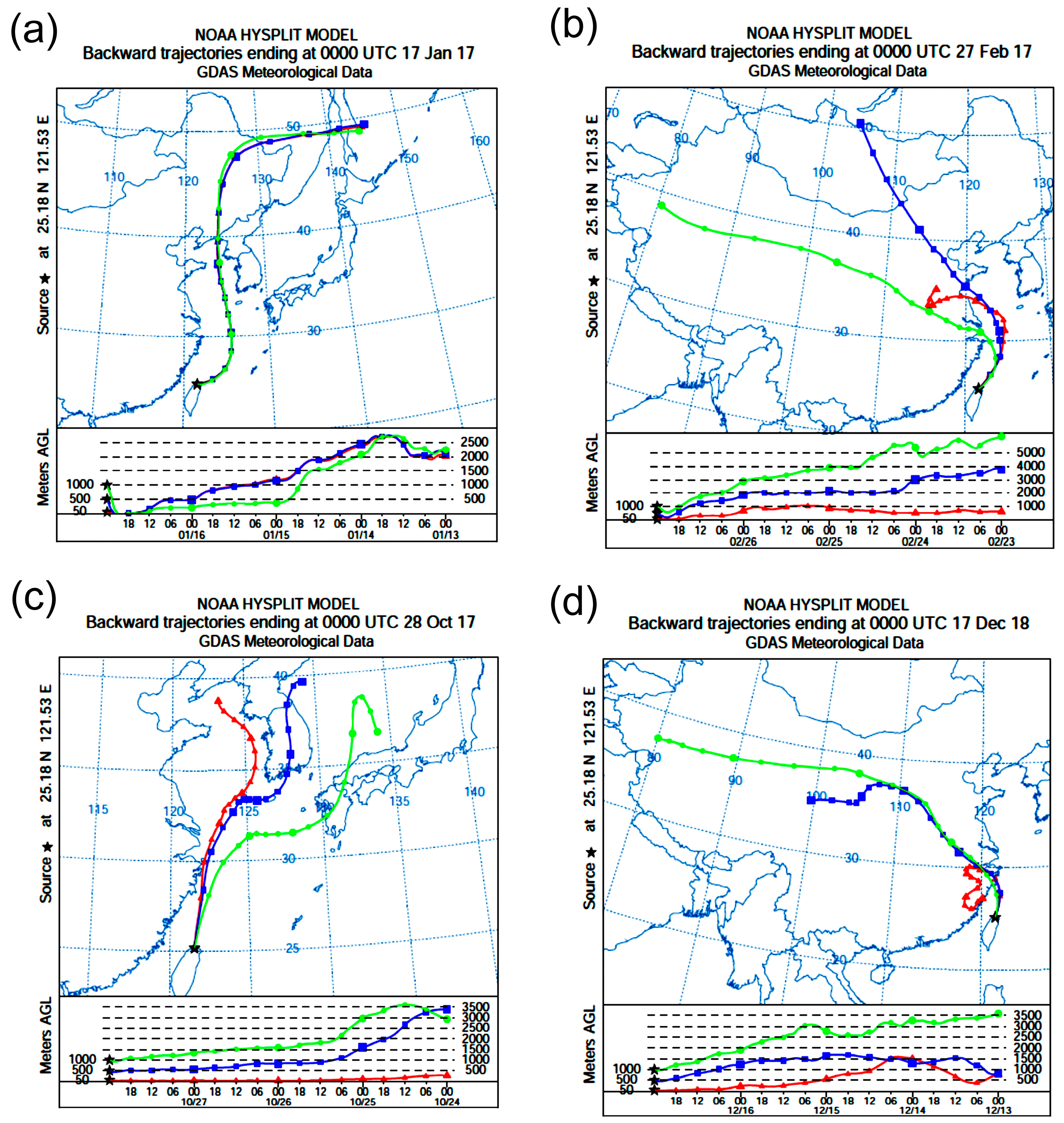
According to Chen and Chen [3], AMBTs were conducted at 100 m, 500 m, and 1000 m above ground level to represent airflow trajectories at surface, middle, and high altitudes, respectively. In this study, the AMBT model was simulated at three different altitudes above ground level: 50 m (red line), 500 m (blue line), and 1000 m (green line), representing low-, mid-, and high-elevation airflows, respectively (see Figure 4). In the figure, the star symbol indicates the research location, with each node covering a six-hour interval. The regional long-range pollution information obtained at each altitude was then classified into the three regions outlined in Figure 1: Region C, Region R, and Region S.

Since rainwater pH values are only available on rainy days, this study estimates air mass back trajectories for 2035 rainy days. The air quality and meteorological data associated with these days are categorized according to the height levels (50, 500, and 1000 m). The classification of these trajectories is based on the regional zones (C, R, and S Regions). Subsequently, machine learning models are established for each classified region, resulting in the creation of the ANN_AMBT integral model. This model integrates ANN with AMBT data to enhance the accuracy of acid rain pH predictions.

Table 5. Optimal models and parameter settings for ANN_AMBT with different altitudes.

ANN Model	Altitude of AMBT	Parameters Tuned	RMSE
DNN	50 m	Learning rate (LR) = 0.1, No. of hidden layers (NHL) = 3, No. of neurons per hidden layer (NNE) = 10	0.386
DNN	500 m	LR = 0.1, NHL = 1, NNE = 40	0.404
DNN	1000 m	LR = 0.1, NHL = 1, NNE = 90	0.395
LSTM	50 m	NHL = 1, NNE = 10	0.360
LSTM	500 m	NHL = 1, NNE = 10	0.401
LSTM	1000 m	NHL = 1, NNE = 30	0.357

presents the best parameter combinations for DNN and LSTM models after parameter adjustment, using air mass trajectory data obtained from different heights. The results show that using air mass trajectory classification data results in lower errors compared to using only ground monitoring parameters. Additionally, at height levels of 50, 500, and 1000 m, the LSTM model consistently achieves smaller RMSE errors compared to the DNN model.

5. Simulation and Discussion

5.1. Simulation

This study conducted simulation experiments on a test dataset using the various models adjusted in the previous section. The results of the evaluation metrics are summarized in

Table 6. Evaluation results of simulation experiments.

DNN Model	MAPE	C.V.	TS	LSTM Model	MAPE	C.V.	TS
No_AMBT	8.88%	9.40%	0.088	No_AMBT	7.97%	9.03%	−0.098
AMBT_50m	8.00%	9.14%	0.061	AMBT_50m	7.35%	8.41%	0.013
AMBT_500m	8.02%	9.18%	−0.051	AMBT_500m	7.37%	8.36%	0.022
AMBT_1000m	8.38%	9.37%	−0.074	AMBT_1000m	7.41%	8.55%	0.011

. As shown in the table, the comparison of the three evaluation indicators reveals the following:

• Models with MAPE < 10% are generally considered acceptable, with values closer to 0% indicating better performance. In a comparison across different models (both DNN and LSTM), all models fall below the 10% threshold. LSTM models, in particular, consistently show lower MAPE values compared to DNN models, indicating better predictive accuracy.
• A higher C.V. typically indicates greater dispersion in the data and higher prediction risk, while a lower C.V. signifies more stable predictions. Results show that the LSTM models have the smallest C.V. among all models, demonstrating better prediction stability.
• Positive TS values indicate that actual values are greater than predicted values, while negative values indicate the opposite. A TS value close to 0 suggests good prediction performance. Both DNN and LSTM models show acceptable TS values, with LSTM models exhibiting slightly better results.

Overall, the evaluation shows that both DNN and LSTM models have acceptable performance, with LSTM models generally outperforming DNN models in terms of MAPE, C.V., and TS.

As the literature indicates, during winter in northern Taiwan, the influence of the continental high-pressure system leads to northeast winds with relatively strong wind speeds. The main pollutants are not only from local emissions but also include contributions from cross-border transmission, resulting in higher pollutant concentrations. When foreign pollutants are carried by northeast winds, severe acid rain events may occur.

In this study, Table 6 shows that the MAPE and C.V. indicators for the ANN-based models with trajectory information at altitudes of 50 m, 500 m, and 1000 m perform better compared to the models without trajectory information (No_AMBT). This demonstrates that the air mass back trajectory (AMBT) model provides valuable information on foreign pollutants, reducing prediction errors for acid rain.

Furthermore, a comparison of the models using trajectories at three different altitudes (surface 50 m, mid-altitude 500 m, and high-altitude 1000 m) reveals that the 50 m and 500 m models provide more useful information for simulating acid rain scenarios than the 1000 m model. This suggests that lower and mid-altitude trajectories may offer more relevant data for accurate acid rain predictions.

According to Taiwan’s MOE, “acid rain” is defined as rainwater with a pH value of less than 5.0. The experimental data in this study show that severe acid rain events at the Yangmingshan monitoring station predominantly occur in the winter months (approximately from November to February). The four most severe acid rain events in the study’s testing data are as follows: 17 January 2017 (pH = 3.6), 27 February 2017 (pH = 3.42), 28 October 2017 (pH = 3.65), and 17 December 2018 (pH = 3.65).

Figure 5 illustrates the trajectory estimation of air masses using the AMBT model on the days of these severe acid rain events. The trajectories of the air masses in the four days prior to these events, under the influence of the continental high-pressure system, indicate that the wind direction was either northeast or north.

Table 7. Severe acid rain event dates, RMSE prediction errors, and corresponding MIR results relative to the LSTM_No_AMBT model.

Metrics	Model	Dates of Severe Acid Rain Events				Average
		17 January 2017	27 February 2017	28 October 2017	17 December 2018
RMSE	LSTM_No_AMBT	0.456	0.412	0.320	0.444	0.408
	LSTM_AMBT_50m	0.371	0.314	0.272	0.353	0.328
	LSTM_AMBT_500m	0.334	0.303	0.260	0.362	0.315
	LSTM_AMBT_1000m	0.416	0.401	0.309	0.393	0.380
MIR	LSTM_AMBT_50m	22.91	26.42	12.94	24.53	21.70
(%)	LSTM_AMBT_500m	36.53	32.63	17.96	24.55	27.92
	LSTM_AMBT_1000m	9.62	2.64	2.64	12.26	6.79

shows the prediction error results for severe acid rain event dates in the corresponding months, while Figure 6 illustrates the observed values and predicted trends for these months. The results indicate that during the winter season, when severe acid rain is most prevalent, all LSTM models—LSTM_No_AMBT, LSTM_AMBT_50m, LSTM_AMBT_500m, and LSTM_AMBT_1000m—are capable of appropriately simulating the pH values of acid rain. Specifically, the LSTM models integrated with trajectory information outperform the LSTM_No_AMBT model in describing the variation profile of rainwater pH. Additionally, the root mean squared error (RMSE) comparison shows that the LSTM models achieve the smallest errors, with LSTM_AMBT_500m providing the most accurate predictions.

Based on the RMSE results of the LSTM_No_AMBT model, this study defined a “Model Improvement Rate” (abbreviated as MIR) as follows:

$$\mathrm{M}\mathrm{I}\mathrm{R}=\left({\mathrm{R}\mathrm{M}\mathrm{S}\mathrm{E}}_{\mathrm{L}\mathrm{S}\mathrm{T}\mathrm{M}\_\mathrm{N}\mathrm{o}\_\mathrm{A}\mathrm{M}\mathrm{B}\mathrm{T}}-\mathrm{R}\mathrm{M}\mathrm{S}\mathrm{E}\right)/{\mathrm{R}\mathrm{M}\mathrm{S}\mathrm{E}}_{\mathrm{L}\mathrm{S}\mathrm{T}\mathrm{M}\_\mathrm{N}\mathrm{o}\_\mathrm{A}\mathrm{M}\mathrm{B}\mathrm{T}}\times 100\%$$

(8)

After calculation, it was found that, across all severe acid rain events, the LSTM_AMBT_500m model had the highest MIR percentages, ranging from 17.96% to 36.53% (average of 27.92%) (see Table 7). This was followed by the LSTM_AMBT_50m model, with MIR percentages ranging from 12.94% to 26.42% (average of 21.70%). The LSTM_AMBT_1000m model had the lowest MIR percentages, ranging from 2.64% to 12.26% (average of 6.79%).

5.2. Discussion

• Limitation of using AMBT

The AMBT method is widely used in atmospheric science to trace air mass movements and investigate pollution sources or other atmospheric phenomena. While this method provides valuable insights in many studies, its limitations could influence research findings in several ways:

(1)

AMBT relies on numerical simulations to trace air mass movements backward in time. These calculations depend heavily on initial conditions and the accuracy of atmospheric models. Over extended periods, errors in numerical simulations can accumulate, particularly in long-term back trajectory tracking. If models fail to accurately represent atmospheric dynamics, this may lead to incorrect pollution source identification or inaccurate meteorological analysis, affecting the conclusions of the study.

(2)

AMBT depends on precise atmospheric dynamics and meteorological data. Variations in weather patterns (e.g., wind speed, pressure, temperature) directly influence air mass movement. Sudden meteorological changes, such as extreme weather events, may not be fully captured during back trajectory calculations, potentially resulting in misjudgments about pollution sources or atmospheric processes.

(3)

AMBT typically uses mathematical models to predict air mass movements, which inherently involve uncertainties. These uncertainties may be more pronounced in certain regions or conditions, particularly where model resolution is low or data are incomplete. Such discrepancies could reduce the reliability of research findings by failing to accurately reflect real-world conditions.

(4)

AMBT may struggle to account for the influence of complex terrain (e.g., mountains, urban landscapes) on airflows. In such regions, airflow can be significantly affected by local topography, making it difficult to accurately predict air mass trajectories. This limitation could result in substantial errors when studying the transport of local pollutants or other atmospheric processes.

• Insights for public health officials and policymakers

The predictive capabilities of the AI-based models offer a proactive approach to mitigating acid rain by enabling early warnings and informed decision-making. These predictions support timely mitigation strategies, including the following:

(1)

Issuing advisories for at-risk populations, such as children, the elderly, and individuals with respiratory conditions, to limit outdoor activities during periods of high acid rain risk. This helps to reduce potential health impacts associated with exposure.

(2)

Identifying high-risk areas or pollution hotspots allows for the implementation of targeted measures, such as stricter industrial emission regulations, transitioning to clean energy sources, and designing urban green spaces to mitigate environmental degradation.

(3)

Promoting international collaboration to tackle transboundary pollution influenced by seasonal monsoons. This includes sharing data, aligning emission reduction targets, and developing regional agreements to address the broader environmental impacts of acid rain.

6. Conclusions

The study employs advanced artificial intelligence technologies to develop models for estimating acid rain, utilizing machine learning algorithms such as DNN and LSTM neural networks. Given the high levels of industrialization and urbanization in northern Taiwan, combined with the impact of seasonal monsoons bringing foreign pollutants, this region was selected as the focus of the study.

The study area was selected as the Yangming station in the Taipei metropolitan area. Based on the trajectory patterns of pollutant sources, three potential pollution source regions were defined: the mainland China and Japanese archipelago under the northeast monsoon system (Region C), the Philippines and Indochina Peninsula under the southwest monsoon system (Region R), and the Pacific Ocean under the western Pacific high-pressure system (Region S). Data were categorized according to these regions to develop neural network models. The study developed models for air mass sources at three different heights (50 m, 500 m, and 1000 m). Additionally, a benchmark model was established based solely on the attributes of surface monitoring stations, without incorporating AMBT information. In this study, the benchmark model refers to an ANN model that relies exclusively on ground station attributes (LSTM_No_AMBT) and serves as a baseline for comparison.

The research results are as follows:

• ANN Model Results: The use of LSTM networks significantly outperforms DNNs. Since acid rain pH data are discontinuous (monitoring values are only available during rainfall), and considering environmental physical effects (such as rain washout and removal), the occurrence of events before and after does have an impact. Thus, LSTM networks have an advantage in handling data with delay attributes.
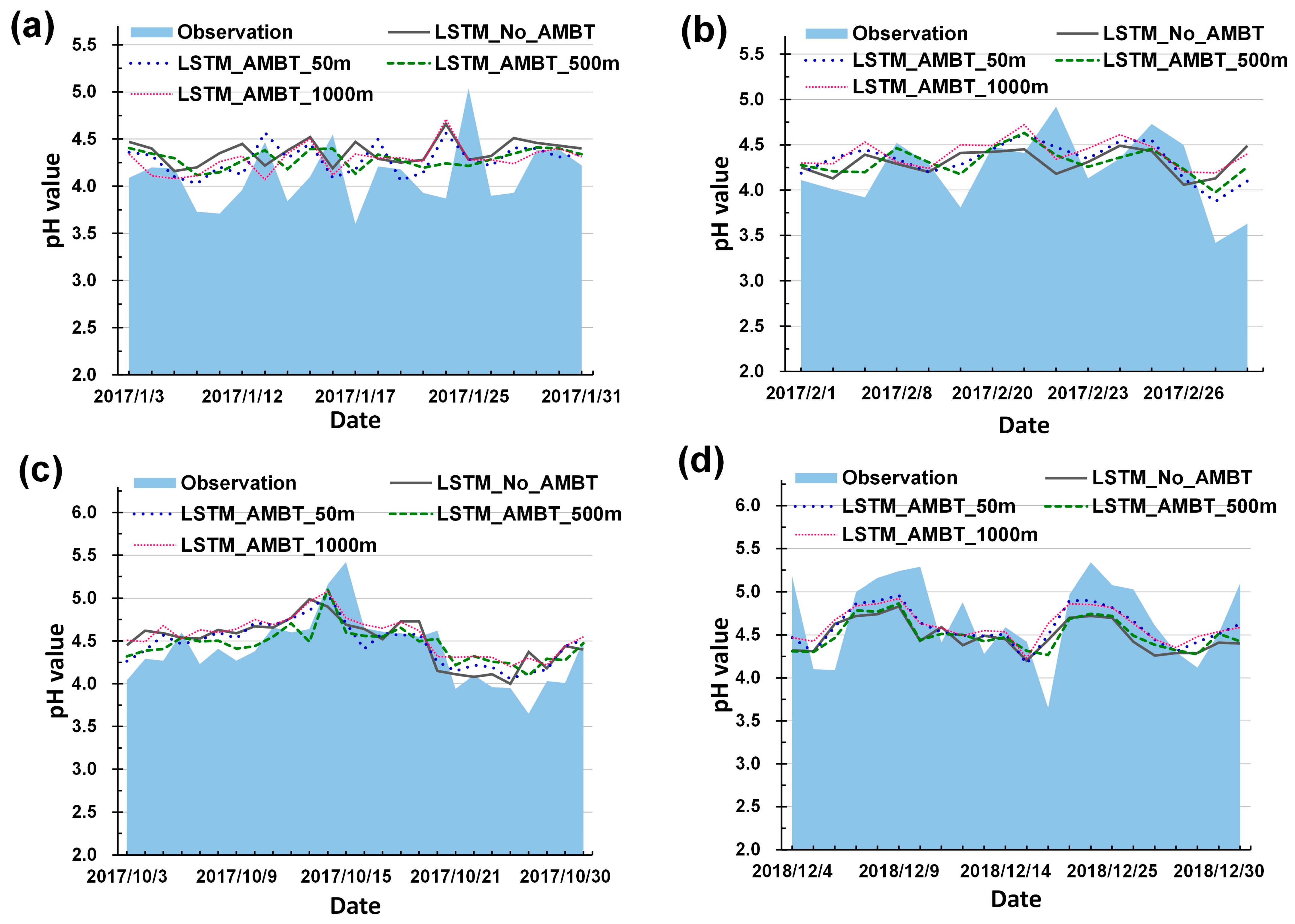
• LSTM_AMBT Models Comparison: The LSTM_AMBT models utilizing three different heights of air mass trajectories (surface 50 m, mid-altitude 500 m, and high-altitude 1000 m)—namely LSTM_No_AMBT, LSTM_AMBT_50m, LSTM_AMBT_500m, and LSTM_AMBT_1000m—demonstrated better performance in describing the variation profile of rainwater pH compared to the model without air mass trajectory information (LSTM_No_AMBT).
• Seasonal Considerations: The Yangming station experiences severe acid rain almost exclusively in winter (December to February). During this season, the trajectory model in the optimal model can consider the pathways of external pollutants due to seasonal variations, thus adapting well to the higher frequency of acid rain occurrences in winter. This highlights the accuracy and feasibility of the ANN_AMBT model in predicting severe acid rain pollution events.

Future recommendations include the following:

• The study used altitudes of 50 m, 500 m, and 1000 m above ground level to represent airflow trajectories at surface, middle, and high altitudes, respectively, and to test suitable heights. While these heights are commonly used, we acknowledge that variations in the selected heights could influence the results. Therefore, we suggest future research to explore the effects of using different heights, such as extending the range to 50 to 1500 m at 100 m intervals, to further validate and refine our findings.
• The study suggests that the model tends to underestimate pH values when the rainwater pH is above 5.15. This is likely due to the lower frequency of such extreme events (severe acid rain) in the collected data (approximately 15% at Yangmingshan station). This discrepancy affects the pH value predictions. Future work should focus on increasing the sample size of severe acid rain events to improve model training and potentially resolve this issue.
• Regarding the proposed methodology, the study utilized year-round data to predict acid rain occurrences. However, the methodology did not specifically develop the ANN_AMBT combination models based on seasonal variations. In the study area, acid rain frequently occurs during the winter season (approximately from November to February in Taiwan). Therefore, it is suggested that future research focuses on developing season-based ANN_AMBT models tailored to periods with a higher likelihood of acid rain occurrence. Such an approach could potentially improve the accuracy of acid rain prediction models.
• In this study, we selected LSTM due to its robustness and widespread validation in time-series tasks, particularly in environmental modeling. This choice aligns well with the size of our dataset and the available computational resources. For future work, we suggest exploring the potential advantages of advanced methods, such as Transformers and hybrid models like convolutional LSTMs, to further improve the accuracy and generalizability of our model.
• As mentioned in Section 5.2, the limitations of AMBT may affect the accuracy and reliability of the study results. To mitigate these impacts, future researchers intending to adopt the methodology presented in this study are advised to carefully select appropriate ANN models and data sources. Additionally, incorporating supplementary methods to validate the AMBT results is recommended to enhance the credibility of the study’s conclusions.