Prediction of Reference Crop Evapotranspiration in China’s Climatic Regions Using Optimized Machine Learning Models

Abstract

The accurate estimation of reference crop evapotranspiration (ET₀) is essential for crop water consumption modeling and agricultural water resource management. In the present study, three bionic algorithms (aquila optimizer (AO), tuna swarm optimization (TSO), and sparrow search algorithm (SSA)) were combined with an extreme learning machine (ELM) model to form three mixed models (AO-ELM, TSO-ELM, and SSA-ELM). The accuracy of the ET₀ estimates for five climate regions in China from 1970 to 2019 was evaluated using the FAO-56 Penman–Monteith (P-M) equation. The results showed that the predicted values of the three mixed models and the ELM model fitted the P-M calculated values well. R² and RMSE were 0.7654–0.9864 and 0.1271–0.7842 mm·d⁻¹, respectively, for which the prediction accuracy of the AO-ELM model was the highest. The performance of the AO-ELM combination5 (maximum temperature (T_max), minimum temperature (T_min), total solar radiation (R_s), sunshine duration (n)) was most significantly improved on the basis of the ELM model. The prediction accuracy for the stations in the plateau mountain climate (PMC) region was the best, while the prediction accuracy for the stations in the tropical monsoon climate region (TPMC) was the worst. In addition to the wind speed (U₂) in the temperate continental climate region (TCC)—which was the largest variable affecting ET₀—n, R_a, and total solar radiation (R_s) in the other climate regions were more important than relative humidity (RH) and wind speed (U₂) in predicting ET₀. Therefore, AO-ELM4 was selected for the TCC region (with T_max, T_min, R_s, and U₂ as inputs) and AO-ELM5 (with T_max, T_min, R_s, and n as inputs) was selected for the TMC, PMC, SMC, and TPMC regions when determining the best model for each climate region with limited meteorological data.

1. Introduction

Reference crop evapotranspiration (ET₀) is the sum of crop transpiration and soil evaporation under conditions of uniform, vigorous growth, complete ground coverage, and adequate water supply. It represents the exchange of gas, energy, and water between the soil, crops, and the atmosphere [1]. The accurate measurement and estimation of regional ET₀ are crucial for simulating crop water consumption, scheduling irrigation, and managing agricultural water resources [2].

There are several methods for calculating ET₀, including the Hargreaves, FAO-56 Penman–Monteith (P-M), and Priestley–Taylor models. The most widely accepted method is the FAO-56 P-M model, recommended by the Food and Agriculture Organization of the United Nations (FAO). This model combines radiation and aerodynamic terms of meteorological factors [3] and has been extensively validated globally [4,5,6]. However, the P-M model requires comprehensive meteorological data, which are often unavailable due to the limited development and insufficient investment in many regions. As a result, empirical models that can accurately estimate ET₀ with minimal input data, such as temperature, radiation, and mass transfer models, have been developed and applied [7].

With the advancement in computing power and the integration of machine learning algorithms in agriculture, researchers have increasingly used various machine learning models to predict ET₀. Examples include the artificial neural network model (ANN) [8,9], support vector machine model (SVM) [10,11,12,13], generalized regression neural network model (GRNN) [14,15], and random forest model (RF) [16,17]. These models have demonstrated high accuracy in predicting ET₀. For instance, Wen et al. [13] used an SVM model to predict ET₀ in arid regions with limited data and found it to outperform three empirical models. Studies have consistently shown that machine learning models provide more accurate ET₀ predictions compared to empirical models [18,19,20,21,22].

Recently, the extreme learning machine model (ELM) has gained popularity due to its fast computation speed and high performance [23,24,25,26,27]. Abdullah et al. [28] found the ELM model to be more efficient and faster than the feedforward backpropagation (FFBP) model and the P-M equation in predicting ET₀ in Iraq. Feng et al. [15,24] and Allan T et al. [12] also reported that the ELM model outperformed other machine learning models.

As research has advanced, scholars have observed that while the extreme learning machine (ELM) model can achieve high accuracy in predicting ET₀, it suffers from issues such as local optimal solutions and slow convergence rates during simulations. These problems reduce the model’s portability across different regions. To address these limitations, researchers have employed various bio-inspired algorithms to optimize the initial weights and thresholds of the ELM model. This optimization aims to mitigate existing model issues, further enhance prediction accuracy, and improve overall predictive performance [8,29]. For instance, Liu et al. [30] employed a hybrid model combining ELM with a genetic algorithm (GA-ELM) to forecast ET₀ in southwestern China. Their findings indicated that the GA-ELM model outperformed both the standalone ELM and empirical models during both training and testing phases. Similarly, Zhu et al. [31] compared the PSO-ELM model with the ELM, ANN, and RF models and six empirical models based on three input modes of radiation, temperature, and mass transfer and found that the machine learning model had more accurate ET₀ predictions than the empirical models, with the PSO-ELM model surpassing other machine learning approaches in performance.

Although many studies have demonstrated that combining the ELM model with bio-inspired algorithms can yield excellent predictions of ET₀, these applications have largely been limited to traditional optimization algorithms such as genetic algorithm (GA), particle swarm optimization (PSO), and whale optimization algorithm (WOA). Over time, several novel bio-inspired algorithms have emerged, including tuna swarm optimization (TSO) [32], aquila optimizer (AO) [33], and sparrow search algorithm (SSA) [34]. However, due to the scarcity of research on the application of these new algorithms in various climate regions across China, their performance remains largely unexplored. Consequently, there are insufficient data to assess the advantages and limitations of these algorithms. To address this gap, the current study proposes the integration of three novel bio-inspired algorithms—TSO, AO, and SSA—with the ELM model. The resulting hybrid algorithms, TSO-ELM, AO-ELM, and SSA-ELM, are applied to simulate and predict the ET₀ at 20 meteorological stations across five distinct climate regions in China, covering the period from 1970 to 2019.

This study aims to combine three new bionic algorithms (TSO, AO, and SSA) with the ELM model to simulate and predict ET₀ across 20 meteorological stations in five Chinese climate regions from 1970 to 2019. The primary objectives are as follows: (1) to analyze the performance of these models under different meteorological factors; (2) to compare the prediction accuracy of the TSO-ELM, AO-ELM, and SSA-ELM models with the standard ELM model; and (3) to recommend reliable forecasting models and meteorological factor input combinations for different Chinese climate regions.

2. Materials and Methods

2.1. Experimental Site

China’s diverse climate is categorized into five distinct climatic regions based on variations in temperature, altitude, and precipitation (Figure 1). These regions include the temperate continental climate region (TCC), temperate monsoon climate region (TMC), plateau mountain climate region (PMC), subtropical monsoon climate region (SMC), and tropical monsoon climate region (TPMC) [35]. The TCC and PMC regions are characterized as arid and semi-arid, with average annual precipitation levels of 285 mm and 382 mm, respectively. The average annual evaporation in these regions is 2148 mm for the TCC region and 1883 mm for the PMC region. In contrast, the TMC region is classified as sub-humid, with an average annual precipitation of 648 mm and an average annual evaporation of 1475 mm. The SMC and TPMC regions are considered humid, with annual precipitation levels of 1538 mm and 1964 mm, respectively. The average annual evaporation in these humid regions is 1545 mm for the SMC region and 1175 mm for the TPMC region.

2.2. Data Collection and Analysis

This study selected 20 representative weather stations with comprehensive and easily accessible meteorological data to capture the climatic characteristics of each region. The selected data spanned from 1970 to 2019 and included the following meteorological variables as input factors for analysis: daily maximum/low temperature (T_max/T_min), atmospheric relative humidity (RH), wind speed at a height of 2 m (U₂), sunshine hours (n), total solar radiation (R_s) and atmospheric radiation (R_a). The performance of a hybrid machine learning model, optimized through various bionic algorithms, was evaluated using these input factors.

Table 1. Geographical locations of selected weather stations and daily mean values of meteorological data from 1970 to 2019.

Climate Regions	Station	Latitude (N)	Longitude (E)	Elevation (m)	Tmax (℃)	Tmin (℃)	N (h)	RH (%)	U2 (m·s−1)	Rs (MJ m−2·d−1)	Ra (MJ m−2·d−1)
TCC	Kuerle	41.75	86.17	937	18.31	6.09	7.89	45.21	1.30	15.97	27.61
	Kashi	39.47	75.99	1281	18.49	6.02	7.71	49.93	1.01	16.32	28.41
	Jiuquan	39.75	98.51	1476	15.07	1.24	8.42	47.10	1.25	16.91	28.31
	Huhehaote	40.81	111.62	1074	13.46	0.93	7.72	52.16	1.06	15.96	27.93
TMC	Changchun	43.83	125.29	215	11.34	0.83	7.14	62.76	2.07	14.56	26.78
	Zhengzhou	34.72	113.64	107	20.40	9.89	5.80	64.29	1.39	14.77	30.02
	Linxia	35.60	103.21	1882	14.49	1.69	6.66	66.33	0.71	15.60	29.75
	Luochuan	35.76	109.43	1166	15.63	4.83	6.89	61.76	1.19	15.85	29.69
PMC	Xining	36.65	101.77	2249	14.05	0.08	7.27	56.24	0.82	16.14	29.42
	Linzhi	29.64	94.36	3100	16.29	4.05	5.48	63.19	0.94	14.90	31.57
	Naqu	31.48	92.05	4500	7.13	−7.73	7.58	51.76	1.48	17.38	31.04
	Changdu	31.14	97.18	3244	16.82	0.93	6.56	50.31	0.64	16.15	31.14
SMC	Wuhan	30.60	114.03	48	21.46	13.22	5.26	77.02	1.08	14.76	31.30
	Guangzhou	23.16	113.27	21	26.56	18.99	4.57	76.98	1.02	14.57	33.23
	Guiyang	26.68	106.62	1100	19.63	12.12	3.15	77.53	1.26	12.47	32.41
	Dujiangyan	30.99	103.65	1019	19.28	12.65	2.52	79.68	0.66	11.15	31.18
TPMC	Haikou	20.03	110.33	15	28.11	21.55	5.61	83.18	1.53	16.50	33.93
	Dongfang	19.10	108.65	73	28.71	22.26	7.07	78.78	2.42	18.61	34.10
	Lancang	22.56	99.93	1054	27.45	14.69	5.91	77.41	0.48	16.45	33.38
	Zhanjiang	21.27	110.37	23	26.84	20.76	5.24	81.89	1.62	15.80	33.69

presents the geographical coordinates (longitude and latitude), altitude, and multi-year average meteorological data for the selected weather stations. The wind speed at a height of 10 m (U₁₀) was converted to a 2 m height equivalent (U₂) using established wind profile relationships. The average temperature (T_mean) was calculated as the average of T_max and T_min [1]. The meteorological data utilized in this study were sourced from the National Meteorological Information Center–China Meteorological Data Network “https://data.cma.cn/ (accessed on 15 July 2023)”, ensuring data authenticity and validity.

In cases where meteorological data were missing, an interpolation method was employed to estimate and fill in the missing records, thereby maintaining data integrity. Given the extensive time span and volume of the data, the meteorological records from 1970 to 2019 were divided into training and test datasets. The training dataset comprised 40 years of meteorological data, whereas the test dataset included 10 years of data. This division allowed for a robust assessment of the model’s performance across different temporal scales.

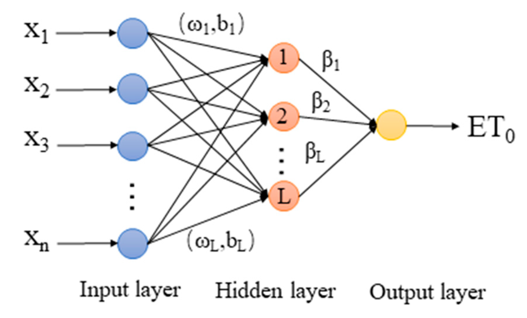
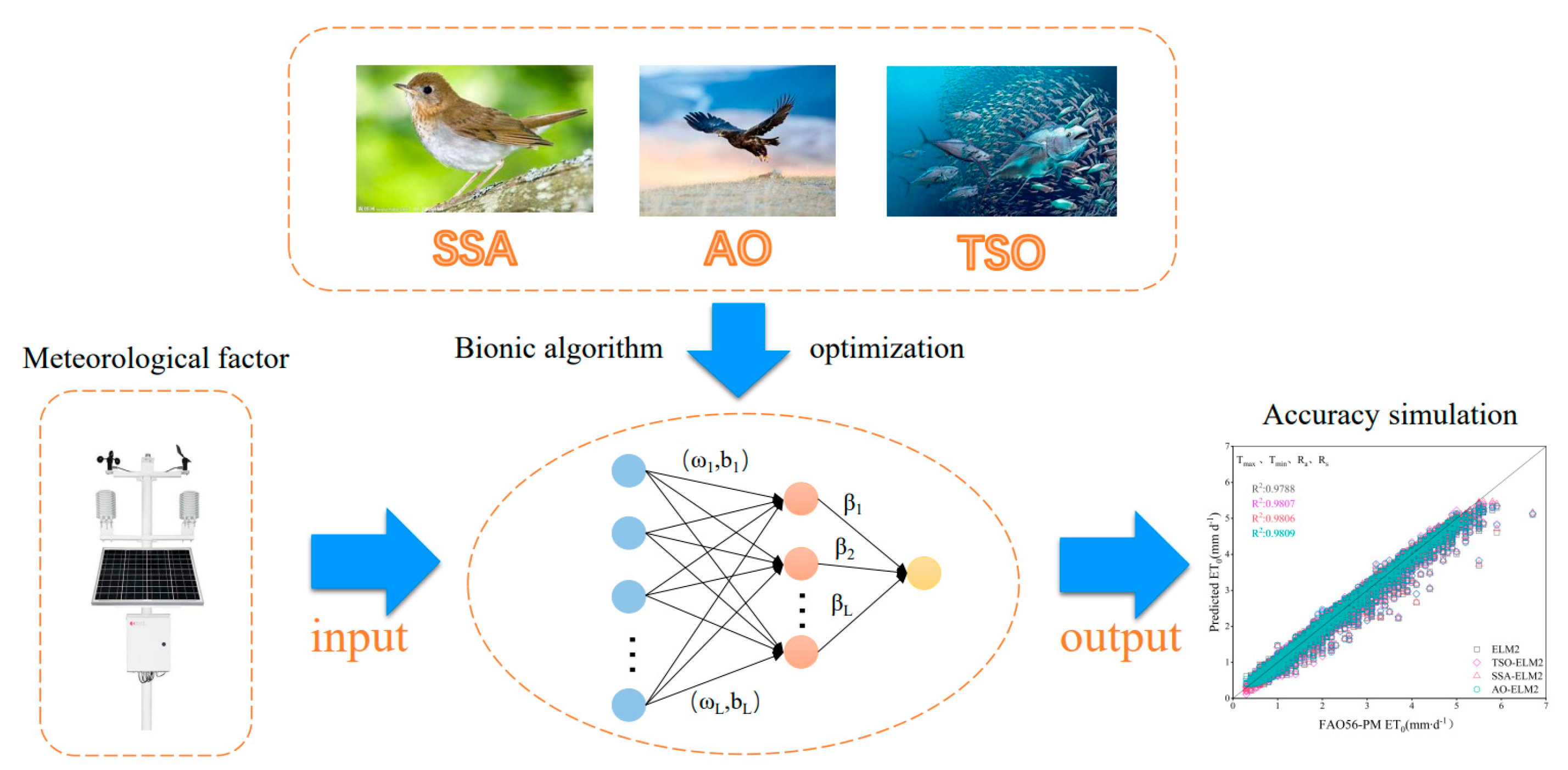
2.3. Extreme Learning Machine Model (ELM)

To address the challenges of slow convergence and lengthy iteration times associated with traditional machine learning models, the extreme learning machine (ELM) proposes a learning algorithm based on a single hidden layer feedforward neural network [36]. This algorithm requires the user only to specify the number of hidden layer nodes, randomly generate all the parameters of the hidden layer, and employ the least squares method to determine the weights of the output layer [37]. The ELM algorithm is favored by many researchers due to its characteristics, including short computation times, strong nonlinear approximation capabilities, and robust learning performance.

Figure 2 illustrates the topology of the ELM, which consists of an input layer, a hidden layer, and an output layer. In this network model, the input sample is represented by x, and the output of the hidden layer is denoted as H (x). The calculation formula for the output H (x) of the hidden layer is expressed as follows:

$$\mathrm{H}\left(\mathrm{x}\right)=\left[{\mathrm{h}}_1\left(\mathrm{x}\right),\dots ,{\mathrm{h}}_{\mathrm{L}}\left(\mathrm{x}\right)\right]$$

(1)

The input value is multiplied by the corresponding weight, adjusted by a bias term, and subsequently processed through a nonlinear function node to obtain the hidden layer’s output. Here, h_i (x) denotes the output of the i-th hidden node, which can be formulated as follows:

$${\mathrm{h}}_{\mathrm{i}}\left(\mathrm{x}\right)=\mathrm{g}\left({\mathrm{w}}_{\mathrm{i}},{\mathrm{b}}_{\mathrm{i}},\mathrm{x}\right)=\mathrm{g}({\mathrm{w}}_{\mathrm{i}}\mathrm{x}+{\mathrm{b}}_{\mathrm{i}}{),\mathrm{w}}_{\mathrm{i}}\in {\mathrm{R}}^{\mathrm{D}},{\mathrm{b}}_{\mathrm{i}}\in \mathrm{R}$$

(2)

In this expression, $\mathrm{g}\left({\mathrm{w}}_{\mathrm{i}},{\mathrm{b}}_{\mathrm{i}},\mathrm{x}\right)$ serves as the activation function. For this study, the Sigmoid function is employed, defined as:

$$\mathrm{g}\left(\mathrm{x}\right)={\displaystyle \frac{1}{1+{\mathrm{e}}^{-\mathrm{x}}}}={\displaystyle \frac{{\mathrm{e}}^{\mathrm{x}}}{{\mathrm{e}}^{\mathrm{x}}+1}}$$

(3)

Finally, the output from the output layer is given by:

$${\mathrm{f}}_{\mathrm{L}}\left(\mathrm{x}\right)={\sum }_{\mathrm{i}=1}^{\mathrm{L}}{\mathsf{\beta }}_{\mathrm{i}}{\mathrm{h}}_{\mathrm{i}}\left(\mathrm{x}\right)=\mathrm{H}\left(\mathrm{x}\right)\mathsf{\beta }$$

(4)

2.4. Novel Bionic Algorithm

In this study, the sparrow search algorithm, tuna swarm optimization algorithm, and Skyhawk search algorithm were employed to optimize the initial weights and thresholds of the ELM model. The primary aim of this optimization is to enhance the overall performance of the ELM model.

Figure 3 illustrates the entire process of the ELM model, which includes the input of meteorological factors, the optimization stage utilizing the three bionic algorithms, and the final model output. The schematic principles of the three bionic algorithms are further detailed in Figure 4.

2.4.1. Sparrow Search Algorithm (SSA)

The sparrow search algorithm was first proposed by Xue Jiankai in 2020 [34]. Inspired by the predation and anti-predation behaviors of sparrows to attain the optimal position, the individuals within the population are categorized into two roles: discoverers and followers. This categorization mimics the real predation scenario to search for the optimal value. The search process is conducted through the following steps:

• Initialization of sparrow population:

Suppose there are n sparrows in a predator population, with the initial population F_X represented as a matrix of fitness values:

$${\mathrm{F}}_{\mathrm{X}}=\mathrm{f}\left[\mathrm{X}\right]=\left[\begin{array}{ccccc}\mathrm{f}\left(\right[{\mathrm{x}}_{1,1}& {\mathrm{x}}_{1,2}& \cdots & \cdots & {\mathrm{x}}_{1,\mathrm{d}}\left]\right)\\ \mathrm{f}\left(\right[{\mathrm{x}}_{2,1}& {\mathrm{x}}_{2,2}& \cdots & \cdots & {\mathrm{x}}_{2,\mathrm{d}}\left]\right)\\ ⋮& ⋮& ⋮& ⋮& ⋮\\ \mathrm{f}\left(\right[{\mathrm{x}}_{\mathrm{n},1}& {\mathrm{x}}_{\mathrm{n},2}& \cdots & \cdots & {\mathrm{x}}_{\mathrm{n},\mathrm{d}}\left]\right)\end{array}\right]$$

(5)

The fitness values of the sparrow population are then sorted from largest to smallest to obtain the optimal fitness value of the sparrow. Subsequently, the initially generated sparrow population is updated according to the position of the discoverer, follower, and danger warning. The formulas for these updates are as follows:

2.

Discoverer Update:

$${\mathrm{X}}_{\mathrm{i},\mathrm{j}}^{\mathrm{t}+1}=\left\{\begin{array}{cc}{\mathrm{X}}_{\mathrm{i},\mathrm{j}}^{\mathrm{t}}\cdot \exp ({\displaystyle \frac{-\mathrm{i}}{\mathsf{\alpha }\cdot {\mathrm{iter}}_{\max }}})& \mathrm{if} {\mathrm{R}}_2 < \mathrm{ST}\\ {\mathrm{X}}_{\mathrm{i},\mathrm{j}}^{\mathrm{t}}+\mathrm{Q}\cdot \mathrm{L}& \mathrm{if} {\mathrm{R}}_2\ge \mathrm{ST}\end{array}\right.$$

(6)

3.

Follower Updates:

$${\mathrm{X}}_{\mathrm{ij}}^{\mathrm{t}+1}=\left\{\begin{array}{cc}\mathrm{Q}\cdot \exp \left({\displaystyle \frac{{\mathrm{x}}_{\mathrm{worst}}^{\mathrm{t}} - {\mathrm{x}}_{\mathrm{ij}}^{\mathrm{t}}}{{\mathrm{i}}^2}}\right)& \mathrm{if} \mathrm{i} > \mathrm{n}/2\\ {\mathrm{X}}_{\mathrm{best} }^{\mathrm{t}}+\mid {\mathrm{X}}_{\mathrm{ij}}^{\mathrm{t}} - {\mathrm{X}}_{\mathrm{best}}^{\mathrm{t}}\mid \cdot \mathrm{rand}\left(\right\{-1,1\left\}\right)\cdot \mathrm{L}& \mathrm{otherwise}\end{array}\right.$$

(7)

4.

Danger warning:

$${\mathrm{X}}_{\mathrm{ij}}^{\mathrm{t}+1}=\left\{\begin{array}{cc}{\mathrm{X}}_{\mathrm{best}}^{\mathrm{t}}+\mathsf{\beta }\cdot \mid {\mathrm{X}}_{\mathrm{ij}}^{\mathrm{t}} -{\mathrm{X}}_{\mathrm{best}}^{\mathrm{t}}\mid & \mathrm{if} {\mathrm{f}}_{\mathrm{i}}>{\mathrm{f}}_{\mathrm{g}}\\ {\mathrm{X}}_{\mathrm{ij}}^{\mathrm{t}}+\mathrm{K}\cdot \left({\displaystyle \frac{\mid {\mathrm{X}}_{\mathrm{ij}}^{\mathrm{t}}-{\mathrm{X}}_{\mathrm{worst}}^{\mathrm{t}}\mid }{({\mathrm{f}}_{\mathrm{i}}-{\mathrm{f}}_{\mathrm{w}})+\mathsf{\epsilon }}}\right)& \mathrm{if} {\mathrm{f}}_{\mathrm{i}}={\mathrm{f}}_{\mathrm{g}}\end{array}\right.$$

(8)

2.4.2. Tuna Swarm Optimization (TSO)

The tuna swarm optimization algorithm is a novel optimization structure algorithm proposed in 2021 based on the predation strategy of tuna [32]. Its primary features include simple operation, fewer adjustable parameters, and higher accuracy beyond local optimization.

• Population initialization:

$${\mathrm{X}}_{\mathrm{i}}^{\mathrm{int}}=\mathrm{rand}\cdot (\mathrm{ub}-\mathrm{lb})+\mathrm{lb},\mathrm{i}=1,2,\cdots ,\mathrm{NP}$$

(9)

2.

Spiral predation:

The tuna group forms a spiral state to control the prey within a certain range, thereby achieving efficient predation. According to the spiral predation strategy, its mathematical model is formulated as follows:

$${\mathrm{X}}_{\mathrm{i}}^{\mathrm{t}+1}=\left\{\begin{array}{cc} {\mathsf{\alpha }}_1\cdot \left({\mathrm{X}}_{\mathrm{best}}^{\mathrm{t}}\right.+\mathsf{\beta }\cdot \left|{\mathrm{X}}_{\mathrm{best}}^{\mathrm{t}}\right.-{\mathrm{X}}_{\mathrm{i}}^{\mathrm{t}}\left|\right)+{\mathsf{\alpha }}_2\cdot {\mathrm{X}}_{\mathrm{i}}^{\mathrm{t}},\hfill & \hfill \mathrm{i}=1\\ {\mathsf{\alpha }}_1\cdot \left({\mathrm{X}}_{\mathrm{best}}^{\mathrm{t}}\right.+\mathsf{\beta }\cdot \left|{\mathrm{X}}_{\mathrm{best}}^{\mathrm{t}}\right.-{\mathrm{X}}_{\mathrm{i}}^{\mathrm{t}}\left|\right)+{\mathsf{\alpha }}_2\cdot {\mathrm{X}}_{\mathrm{i}-1}^{\mathrm{t}},\hfill & \hfill \mathrm{i}=2,3,\cdots ,\mathrm{N}\mathrm{P}\end{array}\right.$$

(10)

An optimal random coordinate is randomly generated within the tuna population, which serves as the reference point for the spiral search. The mathematical model is expressed as:

$${\mathrm{X}}_{\mathrm{i}}^{\mathrm{t}+1}=\left\{\begin{array}{cc} {\mathsf{\alpha }}_1\cdot \left({\mathrm{X}}_{\mathrm{rand}}^{\mathrm{t}}\right.+\mathsf{\beta }\cdot \left|{\mathrm{X}}_{\mathrm{rand}}^{\mathrm{t}}\right.-{\mathrm{X}}_{\mathrm{i}}^{\mathrm{t}}\left|\right)+{\mathsf{\alpha }}_2\cdot {\mathrm{X}}_{\mathrm{i}}^{\mathrm{t}},\hfill & \hfill \mathrm{i}=1\\ {\mathsf{\alpha }}_1\cdot \left({\mathrm{X}}_{\mathrm{rand}}^{\mathrm{t}}\right.+\mathsf{\beta }\cdot \left|{\mathrm{X}}_{\mathrm{rand}}^{\mathrm{t}}\right.-{\mathrm{X}}_{\mathrm{i}}^{\mathrm{t}}\left|\right)+{\mathsf{\alpha }}_2\cdot {\mathrm{X}}_{\mathrm{i}-1}^{\mathrm{t}},\hfill & \hfill \mathrm{i}=2,3,\cdots ,\mathrm{N}\mathrm{P}\end{array}\right.$$

(11)

Heuristic algorithms typically begin with a global search and gradually narrow the search scope to a local search. Consequently, as the number of iterations increases, the search of the tuna population shifts from random reference points to precise optimal individuals.

2.4.3. Aquila Optimizer (AO)

The aquila optimizer is a new biological optimization algorithm developed in 2021 based on the hunting behavior of the aquila in nature [33]. It possesses strong optimization capabilities and rapid convergence speed. The algorithm explores the optimal solution through a four-stage optimization process, updating the location in real time, and the search mechanism automatically stops when the desired result is achieved.

First, the position of the population within the search range is initialized:

$${\mathrm{X}}_{\mathrm{ij}}=\mathrm{rand}\times \left(\mathrm{U}{\mathrm{B}}_{\mathrm{j}} -\mathrm{L}{\mathrm{B}}_{\mathrm{j}}\right)+\mathrm{L}{\mathrm{B}}_{\mathrm{j}}, \mathrm{i}=1,2,\dots ,\mathrm{N} \mathrm{j}=1,2,\dots \mathrm{Dim}$$

(12)

• Extended Search (X1):

Aquila hover high in search of prey areas and select the best hunting area in a vertical bent position. Its mathematical model is as follows:

$${\mathrm{X}}_1(\mathrm{t}+1)={\mathrm{X}}_{\mathrm{best}}\left(\mathrm{t}\right) \times \left(1 - {\displaystyle \frac{\mathrm{t}}{\mathrm{T}}}\right)+({\mathrm{X}}_{\mathrm{M}}\left(\mathrm{t}\right) - {\mathrm{X}}_{\mathrm{best}}\left(\mathrm{t}\right)\cdot \mathrm{rand})$$

(13)

2.

Narrowing Down the Search (X2):

When the first stage identifies the prey area, the AO narrowly searches the selected hunting area for the target prey, preparing to attack the targeted prey. Its mathematical model is expressed as:

$${\mathrm{X}}_2\left(\mathrm{t}+1\right)={\mathrm{X}}_{\mathrm{best}}\left(\mathrm{t}\right)\times \mathrm{Levy}\left(\mathrm{D}\right)+{\mathrm{X}}_{\mathrm{R}}\left(\mathrm{t}\right)+(\mathrm{y}-\mathrm{x})\cdot \mathrm{rand}$$

(14)

3.

Expansion Development (X3):

When the prey is locked down, it descends vertically and attacks. The chosen target area in AO is utilized to get close to the prey. Its mathematical model is formulated as:

$$\begin{array}{cc}{\mathrm{X}}_3(\mathrm{t}+1)& =({\mathrm{X}}_{\mathrm{bex}}\left(\mathrm{t}\right)-{\mathrm{X}}_{\mathrm{M}}\left(\mathrm{t}\right))\times \mathsf{\alpha }-\mathrm{rand}+\left(\right(\mathrm{UB}-\mathrm{LB})\times \mathrm{rand}+\mathrm{LB})\times \mathsf{\delta }\end{array}$$

(15)

4.

Scaling Down Development (X4):

When an aquila attacks its prey, it randomly attacks as the prey moves. Its mathematical model is expressed as:

$${\mathrm{X}}_4(\mathrm{t}+1)=\mathrm{QF}\left(\mathrm{t}\right)\times {\mathrm{X}}_{\mathrm{best}}\left(\mathrm{t}\right)-({\mathrm{G}}_1\times \mathrm{X}\left(\mathrm{t}\right)\times \mathrm{rand})-{\mathrm{G}}_2\times \mathrm{Levy}\left(\mathrm{D}\right)+\mathrm{rand}\times {\mathrm{G}}_1$$

(16)

2.5. Refer to Crop Evapotranspiration Calculation Model

2.5.1. FAO-56 Penman–Monteith Equation

In this study, the FAO-recommended Penman–Monteith formula was employed to calculate the evapotranspiration of 20 sites across various climatic regions in China, providing a benchmark for assessing the model’s accuracy [1].

$${\mathrm{ET}}_0={\displaystyle \frac{0.408\mathsf{\Delta }({\mathrm{R}}_{\mathrm{n}} -\mathrm{G})+\mathsf{\gamma }\frac{900}{\mathrm{T}+273}{\mathrm{U}}_2({\mathrm{e}}_{\mathrm{s}} -{\mathrm{e}}_{\mathrm{a}})}{\mathsf{\Delta }+\mathsf{\gamma }(1+0.34{\mathrm{U}}_2)}}$$

(17)

where ET₀ is the reference crop evapotranspiration quantity (mm·d⁻¹); R_n is the net radiation; G is the soil heat flux (MJ m⁻²·d⁻¹); T is the average temperature (℃); e_s is the saturated water pressure (kPa); e_a is the actual water pressure (kPa); Δ is the slope of the saturated water barometric temperature curve (kPa·℃⁻¹); γ is the hygrometer constant (kPa·℃⁻¹); and U₂ is the ground wind speed 2 m high above the ground (m·s⁻¹). The detailed calculation process of parameters has been explained in the paper FAO-56 [1].

2.5.2. Model Accuracy Verification

To more accurately evaluate and quantify the performance and accuracy of the ET₀ model, four evaluation indices—the coefficient of determination (R²), root mean square error (RMSE), normalized root mean square error (NRMSE), and mean absolute error (MAE)—were employed in this study. Their mathematical expressions are as follows:

$${\mathrm{R}}^2={\displaystyle \frac{{\left[{\sum }_{\mathrm{i}=1}^{\mathrm{n}}({\mathrm{X}}_{\mathrm{i}} -\stackrel{\mathrm{‾}}{\mathrm{X}}\left)\right({\mathrm{Y}}_{\mathrm{i}} -\stackrel{\mathrm{‾}}{\mathrm{Y}})\right]}^2}{{\sum }_{\mathrm{i}=1}^{\mathrm{n}}({\mathrm{X}}_{\mathrm{i}} -\stackrel{\mathrm{‾}}{\mathrm{X}}{)}^2{\sum }_{\mathrm{i}=1}^{\mathrm{n}}({\mathrm{Y}}_{\mathrm{i}} -\stackrel{\mathrm{‾}}{\mathrm{Y}}{)}^2}}$$

(18)

$$\mathrm{RMSE}=\sqrt{{\displaystyle \frac{1}{\mathrm{n}}}{\sum }_{\mathrm{i}=1}^{\mathrm{n}}({\mathrm{Y}}_{\mathrm{i}} -{\mathrm{X}}_{\mathrm{i}}{)}^2}$$

(19)

$$\mathrm{NRMSE}={\displaystyle \frac{\sqrt{\frac{1}{\mathrm{n}}\sum _{\mathrm{i}=1}^{\mathrm{n}}{\left({\mathrm{Y}}_{\mathrm{i}} -{ \mathrm{X}}_{\mathrm{i}}\right)}^2}}{\stackrel{\mathrm{‾}}{\mathrm{X}}}} \times 100\%$$

(20)

$$\mathrm{MAE}={\displaystyle \frac{1}{\mathrm{n}}}{\sum }_{\mathrm{i}=1}^{\mathrm{n}}\mid {\mathrm{X}}_{\mathrm{i}} -{\mathrm{Y}}_{\mathrm{i}}\mid$$

(21)

where X_i and Y_i are measured and predicted values, respectively; and $\stackrel{\mathrm{‾}}{\mathrm{X}}$ and $\stackrel{\mathrm{‾}}{\mathrm{Y}}$ are the average of ${\mathrm{X}}_{\mathrm{i}}$ and ${\mathrm{Y}}_{\mathrm{i}}$, respectively. When ET₀ extremes exist in the process of assessing model performance, we should adopt the following strategies to ensure the accuracy and reliability of the results. Firstly, priority should be given to using metrics that are less sensitive to outliers, such as MAE; secondly, in order to gain a more comprehensive understanding of the model performance, we should not rely on only one metric to assess model performance, but should use a combination of multiple metrics, such as R², MAE, RMSE, and NSE; furthermore, before assessing the model, it is very important to carry out appropriate preprocessing and outlier handling of the data, which can help to minimize the impact of outliers on the assessment results.

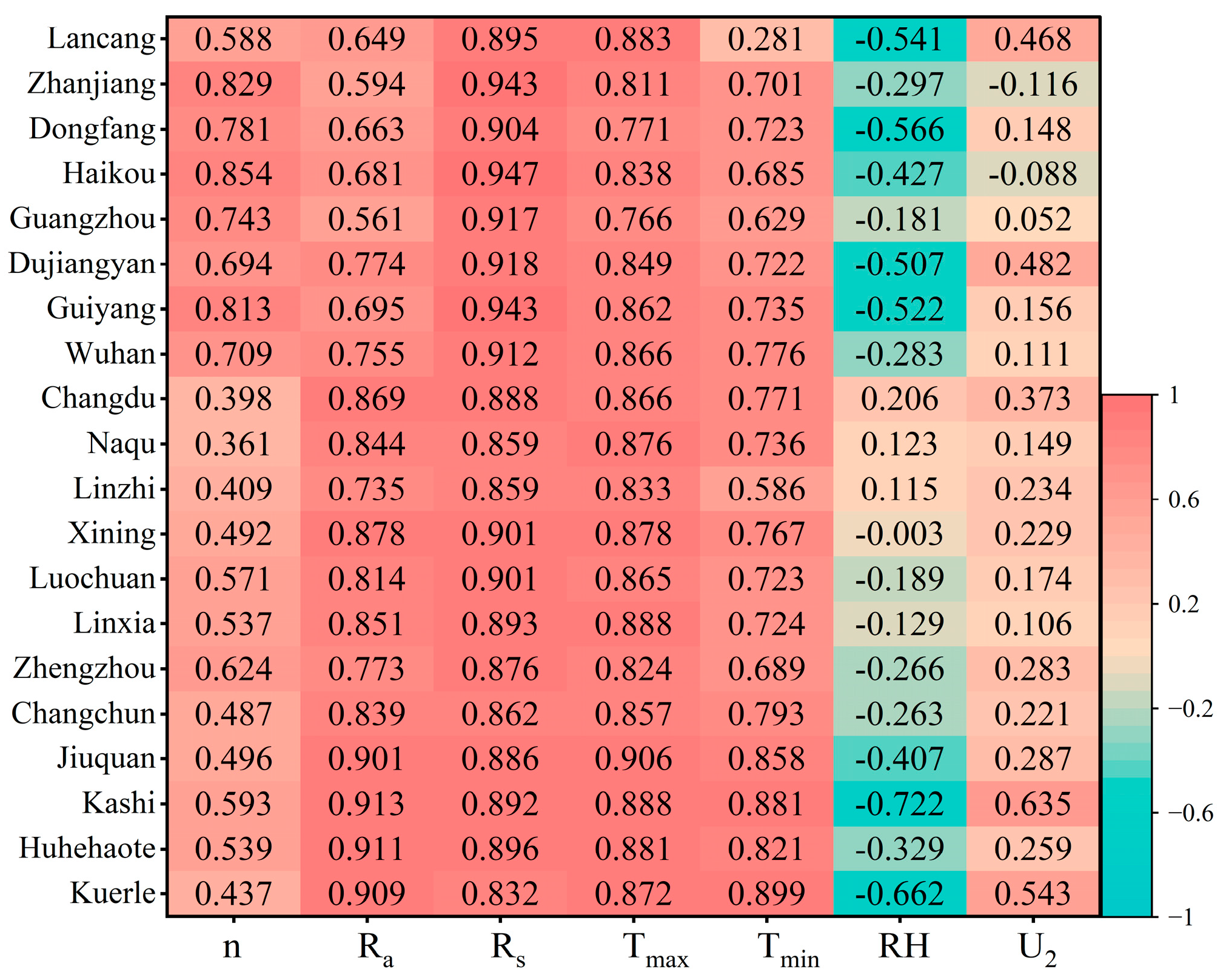
2.6. The Importance of Meteorological Factors for ET₀ as Determined by the Through Analysis Method

Figure 5 illustrates the importance of meteorological factors on ET₀ based on the path coefficient method. The study assessed the impact of seven meteorological factors on ET₀ at 20 stations using the path coefficient method. The results indicate that total solar radiation (Rs) and maximum temperature (T_max) are the most influential factors on ET₀, with importance ranges of 0.832–0.947 and 0.766–0.906, respectively, which are crucial across most meteorological stations. The U₂ factor shows significant importance only at the Kuerle and Kashi stations, while it is less influential at other stations. Additionally, the relative humidity (RH) factor exhibits an inverse effect on ET₀ at most stations, meaning that an increase in humidity leads to a decrease in ET₀. Therefore, the importance of each factor in influencing ET₀ can be ranked as follows: R_s > T_max > R_a > T_min > n > U₂ > RH.

In the present study, seven meteorological factors were combined based on their importance and ease of acquisition. The basic combination included T_max, T_min, and R_s. Additional factors such as R_a, RH, U₂, and n were then added individually to form four combinations. According to the principle of mass transfer, RH and U₂ were further added to the temperature factors to form a total of six input combinations. The detailed meteorological input combinations are presented in

Table 2. Input combinations of meteorological variables for various machine learning models.

Models				Input Combinations
ELM	TSO-ELM	SSA-ELM	AO-ELM
ELM1	TSO-ELM1	SSA-ELM1	AO-ELM1	Tmax, Tmin, Rs
ELM2	TSO-ELM2	SSA-ELM2	AO-ELM2	Tmax, Tmin, Rs, Ra
ELM3	TSO-ELM3	SSA-ELM3	AO-ELM3	Tmax, Tmin, Rs, RH
ELM4	TSO-ELM4	SSA-ELM4	AO-ELM4	Tmax, Tmin, Rs, U2
ELM5	TSO-ELM5	SSA-ELM5	AO-ELM5	Tmax, Tmin, Rs, n
ELM6	TSO-ELM6	SSA-ELM6	AO-ELM6	Tmax, Tmin, RH, U2

.

3. Results and Analysis

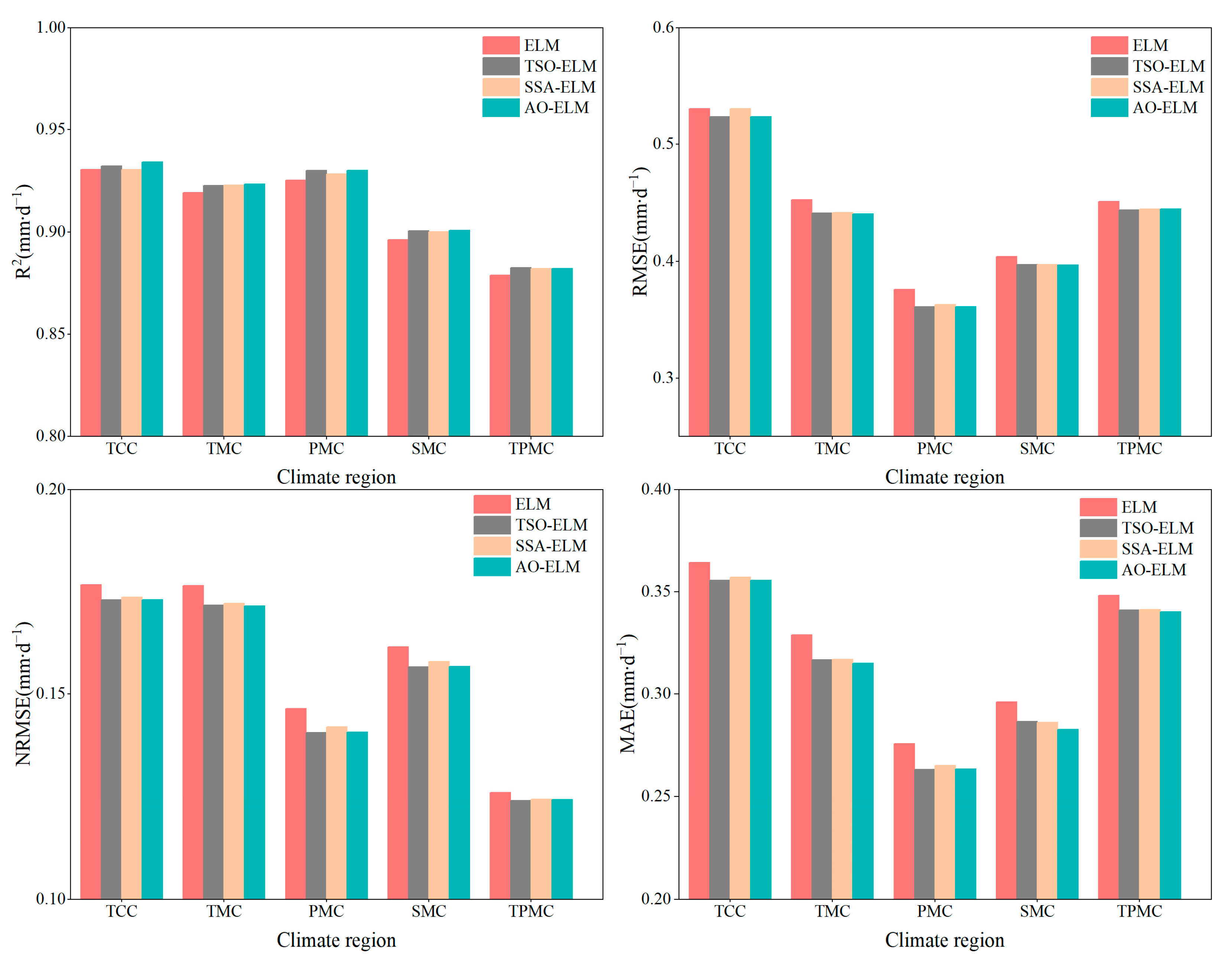
3.1. Comparison of Performance Differences of Machine Learning Models in Different Climate Regions

In this study, four evaluation indicators were used to assess the ET₀ prediction capability of the ELM model and the three hybrid machine learning models (TSO-ELM, SSA-ELM, AO-ELM) across five climate regions in China under various combinations of inputs. The evaluation indicators are shown in Figure 6. It was observed that all four of these models achieved satisfactory prediction accuracy, with the hybrid models demonstrating higher accuracy under the same meteorological input combinations compared to the ELM model. Notably, the combination5 yielded better predictions than the other combinations, while using combination1exhibited the worst performance in terms of R², indicating significant differences in model accuracy across different meteorological input scenarios.

To further evaluate the performance of each model, the statistical indicators from each climate region station during the training stage and the test stage were averaged, with the results presented in

Table 3. Average statistical values of mixed machine learning models with six different input parameters in the training and testing phases of TCC in China.

	Training				Testing
	R2	RMSE	NRMSE	MAE	R2	RMSE	NRMSE	MAE
ELM1	0.9022	0.6259	0.2178	0.4219	0.9046	0.6251	0.2060	0.4265
TSO-ELM1	0.9041	0.6197	0.2155	0.4155	0.9016	0.6402	0.2118	0.4151
SSA-ELM1	0.9038	0.6208	0.2160	0.4163	0.9010	0.6721	0.2123	0.4162
AO-ELM1	0.9043	0.6191	0.2153	0.4144	0.9015	0.6402	0.2117	0.4150
ELM2	0.9304	0.5233	0.1730	0.3592	0.9282	0.5475	0.1807	0.3659
TSO-ELM2	0.9337	0.5136	0.1771	0.3519	0.9280	0.5481	0.1807	0.3628
SSA-ELM2	0.9332	0.5157	0.1778	0.3546	0.9281	0.5478	0.1806	0.3637
AO-ELM2	0.9340	0.5127	0.1768	0.3522	0.9278	0.5489	0.1810	0.3644
ELM3	0.9349	0.5107	0.1773	0.3540	0.9238	0.5632	0.1924	0.3957
TSO-ELM3	0.9370	0.5021	0.1743	0.3466	0.9235	0.5642	0.1851	0.3929
SSA-ELM3	0.9372	0.5016	0.1742	0.3450	0.9150	0.5675	0.1862	0.3952
AO-ELM3	0.9375	0.5002	0.1736	0.3433	0.9230	0.5657	0.1856	0.3916
ELM4	0.9612	0.3794	0.1353	0.2527	0.9607	0.3948	0.1321	0.2720
TSO-ELM4	0.9667	0.3542	0.1259	0.2225	0.9658	0.3724	0.1242	0.2450
SSA-ELM4	0.9669	0.3537	0.1257	0.2214	0.9656	0.3734	0.1245	0.2466
AO-ELM4	0.9671	0.3524	0.1241	0.2205	0.9659	0.3717	0.1240	0.2445
ELM5	0.9317	0.5214	0.1797	0.3596	0.9277	0.5494	0.1812	0.3671
TSO-ELM5	0.9332	0.5154	0.1776	0.3531	0.9284	0.5467	0.1803	0.3620
SSA-ELM5	0.9333	0.5146	0.1777	0.3532	0.9279	0.5504	0.1815	0.3631
AO-ELM5	0.9336	0.5143	0.1773	0.3533	0.9280	0.5481	0.1807	0.3639
ELM6	0.9425	0.4715	0.1667	0.3535	0.9440	0.4818	0.1597	0.3635
TSO-ELM6	0.9463	0.4560	0.1612	0.3430	0.9467	0.4701	0.1560	0.3567
SSA-ELM6	0.9459	0.4578	0.1618	0.3448	0.9461	0.4728	0.1568	0.3583
AO-ELM6	0.9468	0.4538	0.1604	0.3408	0.9472	0.4677	0.1552	0.3545

Note: The best indicators under each combination in the table are highlighted in bold.

,

Table 4. Average statistical values of mixed machine learning models with six different input parameters in the training and testing phases of TMC in China.

	Training				Testing
	R2	RMSE	NRMSE	MAE	R2	RMSE	NRMSE	MAE
ELM1	0.8833	0.5658	0.2173	0.4026	0.8866	0.5426	0.2107	0.3924
TSO-ELM1	0.8869	0.5570	0.2140	0.3940	0.8901	0.5345	0.2076	0.3833
SSA-ELM1	0.8868	0.5573	0.2142	0.3945	0.8905	0.5338	0.2075	0.3838
AO-ELM1	0.8876	0.5555	0.2135	0.3930	0.8903	0.5340	0.2075	0.3844
ELM2	0.9289	0.4387	0.1676	0.3032	0.9458	0.3749	0.1462	0.2671
TSO-ELM2	0.9312	0.4312	0.1647	0.2988	0.9481	0.3666	0.1429	0.2625
SSA-ELM2	0.9311	0.4317	0.1648	0.2988	0.9479	0.3673	0.1432	0.2616
AO-ELM2	0.9319	0.4293	0.1639	0.2966	0.9482	0.3661	0.1426	0.2605
ELM3	0.9254	0.4561	0.1739	0.3259	0.9097	0.4769	0.1836	0.3509
TSO-ELM3	0.9299	0.4370	0.1684	0.3109	0.9092	0.4700	0.1786	0.3423
SSA-ELM3	0.9301	0.4366	0.1682	0.3105	0.9094	0.4799	0.1774	0.3517
AO-ELM3	0.9306	0.4351	0.1677	0.3105	0.9097	0.4743	0.1721	0.3412
ELM4	0.9324	0.4310	0.1690	0.3012	0.9195	0.4589	0.1802	0.3223
TSO-ELM4	0.9341	0.4104	0.1610	0.2763	0.9243	0.4447	0.1746	0.3001
SSA-ELM4	0.9378	0.4139	0.1623	0.2789	0.9241	0.4455	0.1749	0.3026
AO-ELM4	0.9394	0.4083	0.1601	0.2735	0.9249	0.4431	0.1738	0.2987
ELM5	0.9288	0.4391	0.1678	0.3042	0.9455	0.3762	0.1467	0.2676
TSO-ELM5	0.9313	0.4315	0.1649	0.2985	0.9473	0.3695	0.1440	0.2629
SSA-ELM5	0.9310	0.4323	0.1871	0.2992	0.9476	0.3682	0.1436	0.2628
AO-ELM5	0.9322	0.4286	0.1637	0.2962	0.9486	0.3649	0.1423	0.2590
ELM6	0.9215	0.4566	0.1865	0.3522	0.9089	0.4874	0.1919	0.3731
TSO-ELM6	0.9290	0.4352	0.1714	0.3305	0.9181	0.4631	0.1825	0.3505
SSA-ELM6	0.9284	0.4378	0.1720	0.3325	0.9176	0.4644	0.1830	0.3509
AO-ELM6	0.9294	0.4338	0.1708	0.3292	0.9194	0.4595	0.1810	0.3468

Note: The best indicators under each combination in the table are highlighted in bold.

,

Table 5. Average statistical values of mixed machine learning models with six different input parameters in the training and testing stages of PMC in China.

	Training				Testing
	R2	RMSE	NRMSE	MAE	R2	RMSE	NRMSE	MAE
ELM1	0.9018	0.3669	0.1505	0.2734	0.8935	0.4895	0.1658	0.3187
TSO-ELM1	0.9032	0.3638	0.1492	0.2699	0.9017	0.4483	0.1522	0.2950
SSA-ELM1	0.9034	0.3635	0.1491	0.2698	0.8990	0.4503	0.1564	0.2979
AO-ELM1	0.9036	0.3630	0.1489	0.2693	0.9020	0.4440	0.1516	0.2943
ELM2	0.9570	0.2368	0.0973	0.1744	0.9608	0.2594	0.1122	0.2216
TSO-ELM2	0.9619	0.2128	0.0880	0.1717	0.9614	0.2580	0.1117	0.2158
SSA-ELM2	0.9582	0.2336	0.0961	0.1724	0.9613	0.2580	0.1115	0.2155
AO-ELM2	0.9587	0.2321	0.0954	0.1710	0.9618	0.2575	0.1111	0.2149
ELM3	0.9265	0.3182	0.1304	0.2399	0.9219	0.3672	0.1689	0.2721
TSO-ELM3	0.9311	0.3083	0.1260	0.2300	0.9284	0.3507	0.1598	0.2517
SSA-ELM3	0.9306	0.3085	0.1264	0.2309	0.9268	0.3512	0.1608	0.2520
AO-ELM3	0.9315	0.3065	0.1256	0.2287	0.9245	0.3522	0.1614	0.2541
ELM4	0.9344	0.3018	0.1237	0.2127	0.9317	0.3649	0.1589	0.3018
TSO-ELM4	0.9387	0.2920	0.1196	0.2015	0.9358	0.3592	0.1561	0.2954
SSA-ELM4	0.9383	0.2932	0.1201	0.2031	0.9338	0.3619	0.1571	0.3004
AO-ELM4	0.9390	0.2912	0.1193	0.2003	0.9346	0.3619	0.1562	0.2955
ELM5	0.9559	0.2396	0.0985	0.1774	0.9615	0.3313	0.1070	0.2149
TSO-ELM5	0.9580	0.2338	0.0961	0.1722	0.9652	0.3155	0.1017	0.2032
SSA-ELM5	0.9580	0.2342	0.0963	0.1725	0.9638	0.3180	0.1029	0.2049
AO-ELM5	0.9582	0.2125	0.0959	0.1724	0.9650	0.3148	0.1014	0.2028
ELM6	0.8839	0.4036	0.1649	0.3172	0.8825	0.4436	0.1658	0.3248
TSO-ELM6	0.8917	0.3887	0.1588	0.3020	0.8867	0.4354	0.1621	0.3180
SSA-ELM6	0.8903	0.3914	0.1600	0.3037	0.8852	0.4387	0.1635	0.3201
AO-ELM6	0.8921	0.3882	0.1587	0.3009	0.8868	0.4352	0.1617	0.3171

Note: The best indicators under each combination in the table are highlighted in bold.

,

Table 6. Average statistical values of mixed machine learning models with six different input parameters in the training and testing stages of SMC in China.

	Training				Testing
	R2	RMSE	NRMSE	MAE	R2	RMSE	NRMSE	MAE
ELM1	0.8486	0.5191	0.2049	0.3722	0.8326	0.5707	0.2181	0.4119
TSO-ELM1	0.8529	0.5116	0.2019	0.3622	0.8344	0.5659	0.2168	0.4009
SSA-ELM1	0.8533	0.5111	0.2017	0.3628	0.8363	0.5627	0.2152	0.4005
AO-ELM1	0.8534	0.5109	0.2016	0.3619	0.8361	0.5629	0.2159	0.3882
ELM2	0.9678	0.2386	0.0953	0.1639	0.9671	0.2360	0.0891	0.1605
TSO-ELM2	0.9690	0.2346	0.0938	0.1606	0.9678	0.2335	0.0881	0.1608
SSA-ELM2	0.9686	0.2349	0.0939	0.1609	0.9676	0.2344	0.0884	0.1611
AO-ELM2	0.9692	0.2340	0.0936	0.1601	0.9678	0.2341	0.0882	0.1606
ELM3	0.8853	0.4521	0.1778	0.3254	0.8770	0.4450	0.1830	0.3335
TSO-ELM3	0.8941	0.4361	0.1713	0.2818	0.8858	0.4318	0.1744	0.3146
SSA-ELM3	0.8941	0.4359	0.1717	0.3081	0.8866	0.4298	0.1745	0.3082
AO-ELM3	0.8939	0.4365	0.1717	0.3072	0.8851	0.4329	0.1753	0.3076
ELM4	0.8753	0.4754	0.1868	0.3476	0.8632	0.5013	0.1982	0.3546
TSO-ELM4	0.8851	0.4548	0.1788	0.3238	0.8701	0.4853	0.1945	0.3421
SSA-ELM4	0.8845	0.4564	0.1794	0.3254	0.8684	0.4884	0.1960	0.3456
AO-ELM4	0.8859	0.4536	0.1784	0.3222	0.8693	0.4872	0.1956	0.3421
ELM5	0.9679	0.2392	0.0957	0.1649	0.9675	0.2281	0.0937	0.1586
TSO-ELM5	0.9689	0.2347	0.0938	0.1609	0.9705	0.2329	0.0896	0.1539
SSA-ELM5	0.9689	0.2352	0.0948	0.1609	0.9705	0.2320	0.0918	0.1565
AO-ELM5	0.9691	0.2343	0.0937	0.1605	0.9707	0.2304	0.0882	0.1533
ELM6	0.8758	0.4789	0.1889	0.3621	0.8705	0.4425	0.1870	0.3585
TSO-ELM6	0.8850	0.4595	0.1813	0.3477	0.8754	0.4328	0.1775	0.3477
SSA-ELM6	0.8849	0.4596	0.1813	0.3431	0.8719	0.4354	0.1817	0.3460
AO-ELM6	0.8857	0.4583	0.1807	0.3426	0.8764	0.4289	0.1762	0.3435

Note: The best indicators under each combination in the table are highlighted in bold.

and

Table 7. Average statistical values of mixed machine learning models with six different input parameters in the training and testing phases of TPMC in China.

	Training				Testing
	R2	RMSE	NRMSE	MAE	R2	RMSE	NRMSE	MAE
ELM1	0.8047	0.5948	0.1697	0.4685	0.8097	0.5892	0.1647	0.4656
TSO-ELM1	0.8056	0.5881	0.1679	0.4607	0.8140	0.5825	0.1629	0.4578
SSA-ELM1	0.8050	0.5889	0.1681	0.4620	0.8129	0.5843	0.1634	0.4601
AO-ELM1	0.8058	0.5877	0.1678	0.4599	0.8137	0.5830	0.1631	0.4577
ELM2	0.9626	0.2524	0.0712	0.1807	0.9579	0.2765	0.0762	0.2006
TSO-ELM2	0.9653	0.2438	0.0689	0.1726	0.9599	0.2700	0.0745	0.1952
SSA-ELM2	0.9651	0.2444	0.0691	0.1731	0.9598	0.2703	0.0745	0.1954
AO-ELM2	0.9656	0.2427	0.0684	0.1715	0.9601	0.2691	0.0743	0.1942
ELM3	0.8573	0.5025	0.1446	0.3897	0.8637	0.4969	0.1392	0.3823
TSO-ELM3	0.8632	0.4918	0.1416	0.3859	0.8664	0.4920	0.1380	0.3749
SSA-ELM3	0.8625	0.4930	0.1419	0.3799	0.8643	0.4960	0.1391	0.3796
AO-ELM3	0.8639	0.4905	0.1412	0.3767	0.8653	0.4938	0.1386	0.3778
ELM4	0.8148	0.5742	0.1638	0.4511	0.8218	0.5708	0.1594	0.4532
TSO-ELM4	0.8244	0.5593	0.1596	0.4380	0.8311	0.5555	0.1552	0.4397
SSA-ELM4	0.8243	0.5593	0.1423	0.4379	0.8308	0.5561	0.1554	0.4362
AO-ELM4	0.8257	0.5572	0.1591	0.4358	0.8295	0.5584	0.1560	0.4353
ELM5	0.9638	0.2491	0.0704	0.1779	0.9592	0.2725	0.0752	0.1973
TSO-ELM5	0.9649	0.2475	0.0692	0.1735	0.9596	0.2707	0.0747	0.1961
SSA-ELM5	0.9650	0.2449	0.0692	0.1733	0.9600	0.2697	0.0744	0.1946
AO-ELM5	0.9653	0.2427	0.0688	0.1717	0.9601	0.2693	0.0743	0.1948
ELM6	0.8531	0.5098	0.1467	0.3957	0.8609	0.5003	0.1408	0.3905
TSO-ELM6	0.8573	0.5023	0.1446	0.3883	0.8647	0.4936	0.1388	0.3830
SSA-ELM6	0.8578	0.5014	0.1444	0.3876	0.8653	0.4925	0.1386	0.3820
AO-ELM6	0.8587	0.4999	0.1439	0.3859	0.8645	0.4936	0.1389	0.3819

Note: The best indicators under each combination in the table are highlighted in bold.

. The R², RMSE, NRMSE, and MAE values ranged from 0.7654 to 0.9864, 0.1271 to 0.7842 mm∙d⁻¹, 0.0409 to 0.2647, and 0.0886 to 0.5757 mm∙d⁻¹, respectively. Based on the test stage data, the AO-ELM model exhibited the best performance, with R², RMSE, NRMSE, and MAE values of 0.9139, 0.4333 mm∙d⁻¹, 0.1532, and 0.3114 mm∙d⁻¹, respectively. The TSO-ELM and SSA-ELM models followed, while the ELM model showed the poorest performance, with R², RMSE, NRMSE, and MAE values of 0.9089, 0.4429 mm∙d⁻¹, 0.1574, and 0.3227 mm∙d⁻¹, respectively.

The AO, TSO, and SSA models all possess strong global search capabilities, rapid convergence rates, and good robustness, characterized by stable performance across diverse optimization problems and datasets, along with concise algorithmic structures and straightforward implementation. The findings indicate that the three bionic algorithms enhance the ELM model with varying degrees of optimization performance, suggesting a certain level of rationality in the bionic algorithms’ optimization of the ELM model.

Despite the superior performance of all three bionic algorithms, there are notable differences. This is attributed to the AO algorithm’s ability to incorporate global information during the optimization process, allowing the AO-ELM model to more effectively avoid overfitting and thereby exhibit stronger generalization abilities. Consequently, the AO-ELM model maintains higher prediction accuracy when faced with new, unseen data. Although the SSA algorithm is also an effective global optimization method, it may become trapped in local optima when dealing with complex problems, limiting the model’s prediction accuracy. Additionally, the convergence speed of the SSA algorithm may be influenced by the initial population and the number of iterations, impacting training efficiency and prediction performance. In practice, the TSO algorithm may be constrained by problem size and complexity. These advantages enable the AO-ELM model to demonstrate higher prediction accuracy and stability in addressing complex prediction tasks.

In summary, the machine learning models in this study achieved commendable accuracy in simulating and predicting ET₀ across the five climate regions, indicating a strong correlation between the predicted and measured values. Furthermore, the performance of the hybrid models varied, suggesting that the simulation performance of the ELM model was improved to varying extents after optimization by the bionic algorithms.

In the five different climate regions, the PMC stations showed good performance in the test stage (mean R² = 0.9281, RMSE = 0.3653 mm∙d⁻¹, NRMSE = 0.1424, MAE = 0.2668 mm∙d⁻¹). The TPMC sites showed the worst performance (mean R² = 0.8815, RMSE = 0.4461 mm∙d⁻¹, NRMSE = 0.1246, MAE = 0.3427 mm∙d⁻¹). In the five distinct climate regions, the PMC (plateau mountain climate) stations exhibited a strong performance during the testing phase, with a mean R² of 0.9281, RMSE of 0.3653 mm∙d⁻¹, NRMSE of 0.1424, and MAE of 0.2668 mm∙d⁻¹. Conversely, the TPMC (tropical and subtropical monsoon climate) stations demonstrated the weakest performance, with a mean R² of 0.8815, RMSE of 0.4461 mm∙d⁻¹, NRMSE of 0.1246, and MAE of 0.3427 mm∙d⁻¹. PMC regions are typically characterized by intense solar radiation and significant diurnal temperature variations. In contrast, TPMC regions are generally marked by high temperatures, elevated humidity levels, and concentrated, heavy rainfall events. Given that the primary meteorological inputs are temperature and solar radiation, factors such as solar radiation (R_s), temperature (T), and sunshine duration (n) have a more pronounced effect on ET₀ prediction in PMC regions. On the other hand, in TPMC regions, rainfall and humidity play a more critical role. The substantial fluctuations in rainfall and humidity can lead to overfitting or underfitting of the model during training, thereby affecting prediction accuracy.

For instance, Dong et al. [38] reported that four hybrid models based on KNEA (K-Nearest Neighbor Evolutionary Algorithm) performed worst at PMC sites when predicting ET₀ across various climate regions in China. Similarly, Wu et al. [23] found that the prediction accuracy of their optimized model was significantly higher in TMC and SMC regions compared to TCC and PMC regions. The discrepancy between our results and those of previous studies may be attributed to differences in the overall performance of the various hybrid machine learning models, the specific combinations of input factors, and the selection of sites within the same climate regions. It is evident that the prediction accuracy of the same hybrid model can vary depending on the climate region of the station, indicating that local climate and environmental conditions influence model performance.

During the testing phase, scatter plots were generated to compare the predicted values and P-M (Penman–Monteith) measured values for the four machine learning models under different input combinations, using Linxia Station as a representative example (Figure 7). Most data points are closely aligned with the 1:1 line, suggesting that the model’s predicted values are in close agreement with the measured values and indicating a strong correlation. However, it is apparent that varying input combinations affect the accuracy of the ET₀ predictions. The R² values for the combination of two and five variables are consistently higher than those of other combinations, and the scatter plots exhibit less dispersion, indicating a better fit between the predicted and measured values and higher prediction accuracy. In contrast, the scatter plots for the input combination of six variables show a high degree of dispersion and less ideal prediction outcomes, suggesting that while introducing solar radiation (R_a) and sunshine duration (n) as input parameters yields reliable prediction performance, incorporating relative humidity (RH) and wind speed (U₂) tends to degrade the model performance.

These findings are consistent with earlier research, confirming that Ra and n are critical parameters for accurate ET₀ prediction [8,39]. The variation in model performance across different climate regions is closely linked to local climate conditions. Sunshine duration indirectly reflects solar radiation, which provides the necessary energy for evapotranspiration, converting liquid water into water vapor [31]. Additionally, some studies have highlighted solar radiation as the primary factor influencing ET₀ variations in China [40]. This further supports the notion that Ra and n are more critical than RH and U₂ for ET₀ prediction.

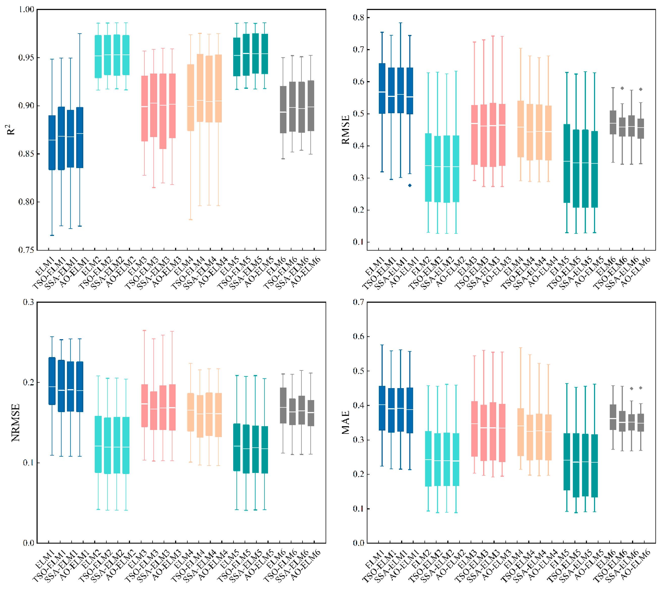
3.2. Comparison of the Stability of Each Machine Learning Model

In general, the four models demonstrated good accuracy across the five climate regions, as shown in Table 3, Table 4, Table 5, Table 6 and Table 7. Figure 8 presents the average RMSE values of the ELM model and the mixed model. The results indicate that the average RMSE values and their growth rates during both the training and testing stages are higher than those observed during the training stage. Fan et al. [25] and Wu et al. [41] also reported similar findings when predicting ET₀. In terms of growth rate, the RMSE growth rates of the three mixed models are higher than that of the ELM model; among them, the AO-ELM model exhibits the largest growth rate (1.5–7.2%), while the ELM model shows the lowest growth rate (0.3–5.9%). However, it is observed that the mixed models all exhibit lower RMSE values than the ELM model in the testing phase. Despite the ELM model having a smaller RMSE increase and a more stable performance, the RMSE value of the AO-ELM model is more satisfactory. Therefore, it is recommended to use the AO-ELM model for simulating and predicting ET₀. Compared to the model performance during the training stage, the model performance at the stations in each climate region declined during the testing stage. The primary reason for this performance difference is the distribution discrepancy between the climatic environment and meteorological data samples during the training and testing stages. McVicar et al. [42] previously discussed in their study that the environment and climate of stations in each region would change over time, resulting in differences in ET₀ prediction accuracy between the two stages.

Figure 9 illustrates the changes in statistical indicators for the mixed model based on the ELM model. As shown in the figure, R² increases by 0.0022–0.5188%, RMSE decreases by −0.0079–3.9794%, NRMSE decreases by 1.3139–4.0016%, and MAE decreases by 1.3139–4.0016% across all the climate regions. This suggests that the mixed model’s performance is improved compared to the ELM model, consistent with the conclusion that the mixed model can achieve better performance in predicting ET₀ than the original model, as noted by Muhammad et al. [43], Zhu et al. [31], and Reham et al. [44]. In particular, in the PMC region, the performance improvement is the most obvious (R² increased by 0.3229–0.5188%, RMSE decreased by 3.9605–3.9794%, NRMSE decreased by 2.9798–4.0016%, MAE decreased by 2.9798–4.0016%). The TSO-ELM model exhibits the best improvement effect (R² increased by 0.5188%, RMSE decreased by 3.9605%, NRMSE decreased by 4.0016%, MAE decreased by 4.5507%). However, the performance improvement at the TCC sites is the poorest, and the RMSE error value of the SSA-ELM model even increases (RMSE increases by 0.0079%), indicating that the optimization effect of the SSA algorithm is not ideal in this area.

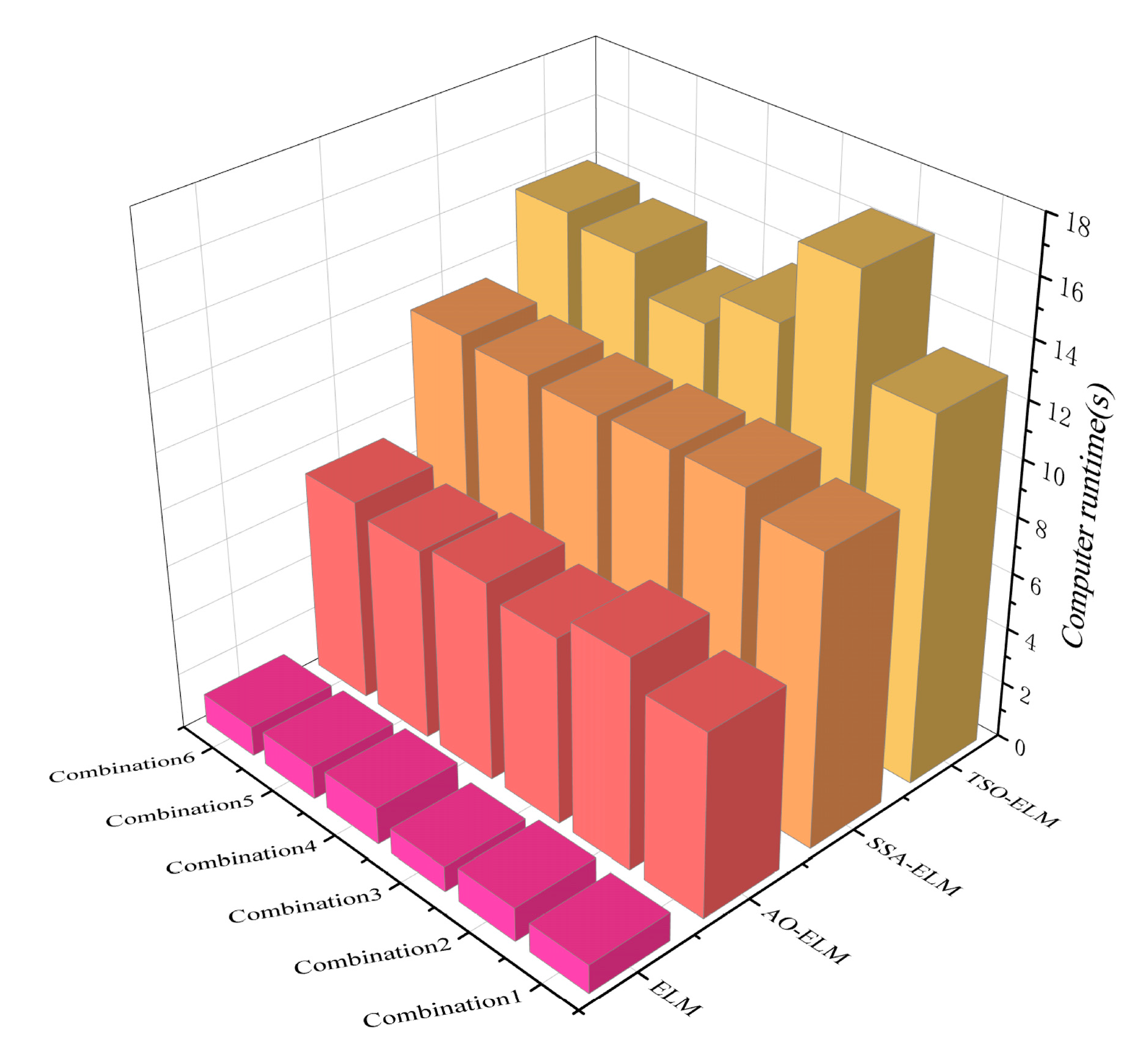
3.3. Comparison of Computational Costs of Various Machine Learning Models

Figure 10 describes the average computational runtime for the four models across combinations of six weather factors. From the figure, it is evident that the ELM model boasts the shortest runtime, which ranges from 0.91 to 1.32 s. The other three hybrid algorithms, however, exhibit longer runtimes, approximately 5.41 to 14.86 times those of the ELM model. This discrepancy is attributed to the larger number of parameters optimized by the hybrid models, which are run using bionic algorithms that necessitate more time to identify the optimal solution. The computational times of the models for various combinations of meteorological factors do not exhibit significant variations. Notably, the TSO-ELM model’s runtime shows slight fluctuations under different combinations. Among the three hybrid algorithms, the AO-ELM model records the shortest runtime. Despite the AO-ELM model’s runtime being increased by 5.41 to 7.34 times compared to the ELM model, its prediction accuracy surpasses that of the ELM model. Given the primary importance of prediction accuracy in estimating ET₀ by a machine learning model, the computational time of the AO-ELM model is deemed acceptable within this context.

3.4. Selection of the Best Model for Each Climate Region

Table 8. Error statistics of the combination of best-performing machine learning models for weather stations in different climate regions in China.

Regions	Station	Model ID	R2	RMSE	MAE	NRMSE
TCC	Kuerle	TSO-ELM4	0.9752	0.3453	0.2202	0.1055
	Kashi	AO-ELM4	0.9725	0.3717	0.2516	0.1163
	Jiuquan	AO-ELM4	0.9628	0.3651	0.2351	0.1267
	Huhehaote	TSO-ELM4	0.9537	0.4003	0.2648	0.1460
TMC	Changchun	TSO-ELM3	0.9307	0.4550	0.3199	0.1852
	Zhengzhou	AO-ELM5	0.9291	0.4485	0.3373	0.1488
	Linxia	AO-ELM5	0.9809	0.1942	0.1290	0.0869
	Luochuan	AO-ELM5	0.9569	0.3311	0.2311	0.1285
PMC	Xining	AO-ELM5	0.9864	0.1655	0.1306	0.0704
	Linzhi	AO-ELM5	0.9471	0.4417	0.2909	0.1231
	Naqu	AO-ELM2	0.9736	0.2219	0.2391	0.1022
	Changdu	AO-ELM5	0.9765	0.2098	0.0929	0.1201
SMC	Wuhan	TSO-ELM2	0.9803	0.2265	0.1542	0.0862
	Guangzhou	TSO-ELM5	0.9567	0.2617	0.1777	0.0865
	Guiyang	AO-ELM5	0.9733	0.2077	0.1365	0.0918
	Dujiangyan	SSA-ELM2	0.9739	0.1921	0.1286	0.0927
TPMC	Haikou	AO-ELM5	0.9532	0.3192	0.2167	0.0898
	Dongfang	SSA-ELM5	0.9387	0.3731	0.2883	0.0886
	Lancang	AO-ELM2	0.9834	0.1271	0.0886	0.0409
	Zhanjiang	AO-ELM5	0.9662	0.2536	0.1825	0.0768

presents the optimal statistical indicator values for the best-performing models derived from meteorological stations across the five climate regions in China, using different meteorological factor inputs (using the testing phase as an example). As indicated in the table, the statistical indices R², RMSE, NRMSE, and MAE range between 0.9291 and 0.9864, 0.1271 and 0.4550 mm·d⁻¹, 0.0886 and 0.3373, and 0.0409 and 0.1825 mm·d⁻¹, respectively, across the climate regions. The AO-ELM model excelled in predictive performance across the most sites (13 sites) among the five climate regions, suggesting that the AO-ELM model can achieve superior prediction performance across a broad range of applications. Our analysis revealed that the hybrid model in the TCC region exhibited the highest prediction accuracy under combination 4. Wind speed directly influences the velocity and direction of water molecule movement on the ground. In conditions of high wind speed, water molecules are more likely to diffuse from the evaporating surface into the atmosphere, thereby accelerating the evaporation rate. Additionally, when constructing the evapotranspiration model, wind speed serves as one of the critical input parameters, and the accuracy and reliability of the wind speed data significantly affect the model’s prediction outcomes. Furthermore, wind speed indirectly impacts the model’s evapotranspiration prediction accuracy by adjusting the model parameters. Given that meteorological stations in this climatic region are situated inland, near deserts and grasslands, characterized by year-round dry, less rainy, and windy conditions, the wind speed’s impact on evapotranspiration becomes more pronounced. This indicates that in this climatic region, ET₀ is more influenced by the U₂ factor, and thus combination 4, which includes the U₂ factor, is more suitable for the TCC region. The other four climate regions exhibited the best performance when using the combination2 and the combination5 as input factors, especially, combination5 notably achieving better prediction accuracy, underscoring the pivotal role of the meteorological factor n in predicting ET₀. This finding aligns with Yan et al.’s [39] conclusion regarding the prediction of ET₀ in arid and humid areas of China, where they observed that wind speed had a greater impact on arid areas, while sunshine duration was more critical in humid areas. In summary, when assessing the predictive performance of different models across various climate regions, the best results are achieved by selecting the most appropriate meteorological input parameters for the local stations.

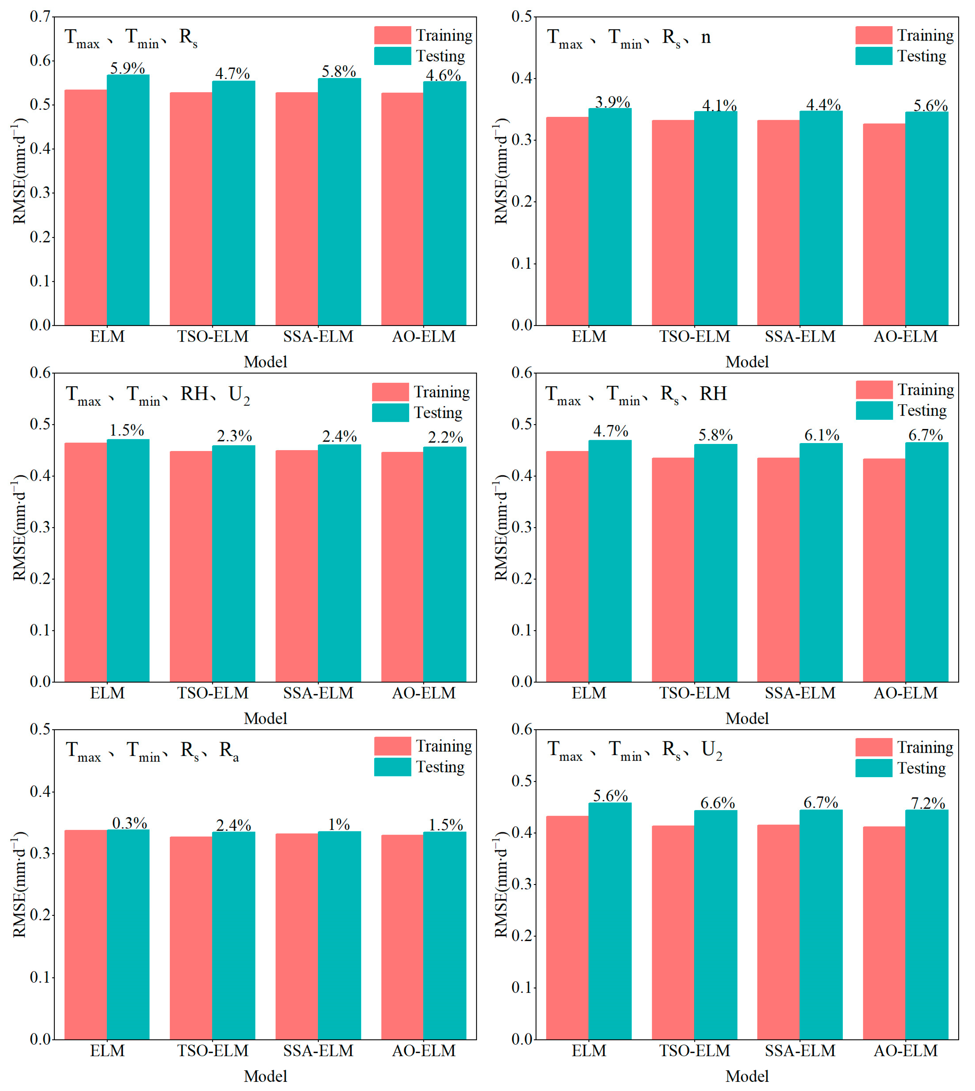
3.5. Improving ET₀ Predictions More Effectively

Although the hybrid algorithm in this study achieved good accuracy, the boosting performance is not satisfactory, for which the prediction of ET₀ can be further improved by the following methods. Firstly, before the introduction of advanced algorithms, it is necessary to carry out pre-processing work on the data, including data missing value processing, outlier detection, etc., which helps to improve the stability and accuracy of the algorithm. Secondly, the appropriate algorithm is selected according to the characteristics of the data and regional variability, and the parameters of the algorithm are tuned. This can be achieved by introducing optimization algorithms to optimize the model parameters; by combining multiple machine learning algorithms, using the advantages of each model to improve the accuracy of the prediction model; or by constructing the ET₀ prediction model through deep machine learning algorithms, integrated learning algorithms, and a series of other methods. After constructing the model, the model needs to be evaluated and verified to ensure its performance in practical applications.

4. Conclusions

In this study, the performance of ELM is optimized using three algorithms: the aquila optimizer (AO), tuna swarm optimization (TSO), and sparrow search algorithm (SSA). The optimized hybrid models, namely AO-ELM, TSO-ELM, and SSA-ELM, along with the standalone ELM model, were simulated to predict the reference evapotranspiration (ET₀) at stations located in various climatic regions across China. The models were trained and tested using daily meteorological data (T_max, T_min, R_s, R_a, RH, U₂, and n) collected from 20 meteorological stations spanning five distinct climatic regions. The models were evaluated with six different combinations of meteorological input factors, and the predicted ET₀ values were compared against those calculated using the FAO-56 Penman–Monteith (PM) equation to assess the degree of fit. The results indicate the following:

(1)

During the testing phase, the three hybrid models demonstrated satisfactory prediction accuracy across different climatic regions. Among them, the AO-ELM model exhibited superior predictive performance compared to the SSA-ELM and TSO-ELM models.

(2)

In scenarios where complete meteorological data are unavailable, the combination of the T_max, T_min, and R_s parameters with U₂ as an input parameter yield better ET₀ predictions in temperate continental monsoon climate regions. Conversely, using n as an input parameter provided satisfactory ET₀ predictions in the other climate regions.

(3)

Stations located in highland mountain climate regions exhibited excellent simulation performance, while those in tropical monsoon climate regions showed the poorest performance. This suggests that local climate conditions significantly influence the overall model performance.

(4)

For model selection, the AO-ELM model demonstrated superior predictive performance when applied on a large scale. Regarding the optimal combination of input parameters, apart from the superior prediction accuracy of the combination4 in the temperate continental monsoon (TCC) region, the combination5 performed better in the remaining four climatic regions. Therefore, AO-ELM4 (utilizing T_max, T_min, R_s, and U₂ as inputs) was chosen for the temperate continental climate (TCC) region, and AO-ELM5 (utilizing T_max, T_min, R_s and n as inputs) was chosen for the tropical monsoon climate (TMC), plateau mountain climate (PMC), subtropical monsoon climate (SMC), and temperate monsoon climate (TPMC) regions when determining the most suitable model for each climatic region with limited meteorological data.

The findings of this study provide valuable insights for predicting ET₀ in diverse climatic regions. However, due to the limited number of bio-inspired algorithms employed in this research, the study has certain limitations. For more in-depth and rigorous research, it is recommended to explore a broader range of meteorological factors, input combinations, or advanced bio-inspired algorithms to develop more reliable methods for ET₀ prediction.

References

1. Allen, R.G. Crop Evapotranspiration-Guidelines for computing crop water requirements. FAO Irrig. Drain. Pap. 1998, 56, 147–151. [Google Scholar]
2. Shiri, J.; Kisi, Ö.; Landeras, G.; López, J.J.; Nazemi, A.H.; Stuyt, L. Daily reference evapotranspiration modeling by using genetic programming approach in the Basque Country (Northern Spain). J. Hydrol. 2012, 414, 302–316. [Google Scholar] [CrossRef]
3. Zhang, Q.; Cui, N.; Feng, Y.; Gong, D.; Hu, X. Improvement of Makkink model for reference evapotranspiration estimation using temperature data in Northwest China. J. Hydrol. 2018, 566, 264–273. [Google Scholar] [CrossRef]
4. Feng, Y.; Jia, Y.; Cui, N.; Zhao, L.; Li, C.; Gong, D. Calibration of Hargreaves model for reference evapotranspiration estimation in Sichuan basin of southwest China. Agric. Water Manag. 2017, 181, 1–9. [Google Scholar] [CrossRef]
5. Yang, Y.; Chen, R.S.; Han, C.T.; Liu, Z.W. Evaluation of 18 models for calculating potential evapotranspiration in different climatic zones of China. Agric. Water Manag. 2021, 244, 106545. [Google Scholar] [CrossRef]
6. Guo, X.H.; Sun, X.H.; Ma, J.J. Prediction of daily crop reference evapotranspiration (ET0) values through a least-squares support vector machine model. Hydrol. Res. 2011, 42, 268–274. [Google Scholar] [CrossRef]
7. Feng, Y.; Jia, Y.; Zhang, Q.; Gong, D.; Cui, N. National-scale assessment of pan evaporation models across different climatic zones of China. J. Hydrol. 2018, 564, 314–328. [Google Scholar] [CrossRef]
8. Gao, L.L.; Gong, D.Z.; Cui, N.B.; Lv, M.; Feng, Y. Evaluation of bio-inspired optimization algorithms hybrid with artificial neural network for reference crop evapotranspiration estimation. Comput. Electron. Agric. 2021, 190, 106466. [Google Scholar] [CrossRef]
9. Ferreira, L.B.; Da Cunha, F.F.; de Oliveira, R.A.; Fernandes, E.I. Estimation of reference evapotranspiration in Brazil with limited meteorological data using ANN and SVM—A new approach. J. Hydrol. 2019, 572, 556–570. [Google Scholar] [CrossRef]
10. Fan, J.L.; Zheng, J.; Wu, L.F.; Zhang, F.C. Estimation of daily maize transpiration using support vector machines, extreme gradient boosting, artificial and deep neural networks models. Agric. Water Manag. 2021, 245, 106547. [Google Scholar] [CrossRef]
11. Mohammadi, B.; Mehdizadeh, S. Modeling daily reference evapotranspiration via a novel approach based on support vector regression coupled with whale optimization algorithm. Agric. Water Manag. 2020, 237, 106145. [Google Scholar] [CrossRef]
12. Tejada, A.T.; Ella, V.B.; Lampayan, R.M.; Reaño, C.E. Modeling Reference Crop Evapotranspiration Using Support Vector Machine (SVM) and Extreme Learning Machine (ELM) in Region IV-A, Philippines. Water 2022, 14, 754. [Google Scholar] [CrossRef]
13. Wen, X.H.; Si, J.H.; He, Z.B.; Wu, J.; Shao, H.B.; Yu, H.J. Support-Vector-Machine-Based Models for Modeling Daily Reference Evapotranspiration With Limited Climatic Data in Extreme Arid Regions. Water Resour. Manag. 2015, 29, 3195–3209. [Google Scholar] [CrossRef]
14. Ladlani, I.; Houichi, L.; Djemili, L.; Heddam, S.; Belouz, K. Modeling daily reference evapotranspiration (ET0) in the north of Algeria using generalized regression neural networks (GRNN) and radial basis function neural networks (RBFNN): A comparative study. Meteorol. Atmos. Phys. 2012, 118, 163–178. [Google Scholar] [CrossRef]
15. Feng, Y.; Peng, Y.; Cui, N.B.; Gong, D.Z.; Zhang, K.D. Modeling reference evapotranspiration using extreme learning machine and generalized regression neural network only with temperature data. Comput. Electron. Agric. 2017, 136, 71–78. [Google Scholar] [CrossRef]
16. Feng, Y.; Cui, N.B.; Gong, D.Z.; Zhang, Q.W.; Zhao, L. Evaluation of random forests and generalized regression neural networks for daily reference evapotranspiration modelling. Agric. Water Manag. 2017, 193, 163–173. [Google Scholar] [CrossRef]
17. Wang, S.; Lian, J.J.; Peng, Y.Z.; Hu, B.Q.; Chen, H.S. Generalized reference evapotranspiration models with limited climatic data based on random forest and gene expression programming in Guangxi, China. Agric. Water Manag. 2019, 221, 220–230. [Google Scholar] [CrossRef]
18. Yang, Y.; Sun, H.W.; Xue, J.; Liu, Y.; Liu, L.G.; Yan, D.; Gui, D.W. Estimating evapotranspiration by coupling Bayesian model averaging methods with machine learning algorithms. Environ. Monit. Assess. 2021, 193, 156. [Google Scholar] [CrossRef]
19. Gul, S.; Ren, J.; Wang, K.; Guo, X. Estimation of reference evapotranspiration via machine learning algorithms in humid and semiarid environments in Khyber Pakhtunkhwa, Pakistan. Int. J. Environ. Sci. Technol. 2023, 20, 5091–5108. [Google Scholar] [CrossRef]
20. Spontoni, T.A.; Ventura, T.M.; Palacios, R.S.; Curado, L.; Fernandes, W.A.; Capistrano, V.B.; Fritzen, C.L.; Pavao, H.G.; Rodrigues, T.R. Evaluation and Modelling of Reference Evapotranspiration Using Different Machine Learning Techniques for a Brazilian Tropical Savanna. Agronomy 2023, 13, 2056. [Google Scholar] [CrossRef]
21. Agrawal, Y.; Kumar, M.; Ananthakrishnan, S.; Kumarapuram, G. Evapotranspiration Modeling Using Different Tree Based Ensembled Machine Learning Algorithm. Water Resour. Manag. 2022, 36, 1025–1042. [Google Scholar] [CrossRef]
22. Nagappan, M.; Gopalakrishnan, V.; Alagappan, M. Prediction of reference evapotranspiration for irrigation scheduling using machine learning. Hydrol. Sci. J. 2020, 65, 2669–2677. [Google Scholar] [CrossRef]
23. Wu, L.F.; Peng, Y.W.; Fan, J.L.; Wang, Y.C.; Huang, G.M. A novel kernel extreme learning machine model coupled with K-means clustering and firefly algorithm for estimating monthly reference evapotranspiration in parallel computation. Agric. Water Manag. 2021, 245, 106624. [Google Scholar] [CrossRef]
24. Feng, Y.; Cui, N.B.; Zhao, L.; Hu, X.T.; Gong, D.Z. Comparison of ELM, GANN, WNN and empirical models for estimating reference evapotranspiration in humid region of Southwest China. J. Hydrol. 2016, 536, 376–383. [Google Scholar] [CrossRef]
25. Fan, J.L.; Yue, W.J.; Wu, L.F.; Zhang, F.C.; Cai, H.J.; Wang, X.K.; Lu, X.H.; Xiang, Y.Z. Evaluation of SVM, ELM and four tree-based ensemble models for predicting daily reference evapotranspiration using limited meteorological data in different climates of China. Agric. For. Meteorol. 2018, 263, 225–241. [Google Scholar] [CrossRef]
26. Feng, Y.; Gong, D.Z.; Mei, X.R.; Cui, N.B. Estimation of maize evapotranspiration using extreme learning machine and generalized regression neural network on the China Loess Plateau. Hydrol. Res. 2017, 48, 1156–1168. [Google Scholar] [CrossRef]
27. Yin, Z.L.; Feng, Q.; Yang, L.S.; Deo, R.C.; Wen, X.H.; Si, J.H.; Xiao, S.C. Future Projection with an Extreme-Learning Machine and Support Vector Regression of Reference Evapotranspiration in a Mountainous Inland Watershed in North-West China. Water 2017, 9, 880. [Google Scholar] [CrossRef]
28. Abdullah, S.S.; Malek, M.A.; Abdullah, N.S.; Kisi, O.; Yap, K.S. Extreme Learning Machines: A new approach for prediction of reference evapotranspiration. J. Hydrol. 2015, 527, 184–195. [Google Scholar] [CrossRef]
29. Chia, M.Y.; Huang, Y.F.; Koo, C.H. Swarm-based optimization as stochastic training strategy for estimation of reference evapotranspiration using extreme learning machine. Agric. Water Manag. 2021, 243, 106447. [Google Scholar] [CrossRef]
30. Liu, Q.S.; Wu, Z.J.; Cui, N.B.; Zhang, W.J.; Wang, Y.S.; Hu, X.T.; Gong, D.Z.; Zheng, S.S. Genetic Algorithm-Optimized Extreme Learning Machine Model for Estimating Daily Reference Evapotranspiration in Southwest China. Atmosphere 2022, 13, 971. [Google Scholar] [CrossRef]
31. Zhu, B.; Feng, Y.; Gong, D.Z.; Jiang, S.Z.; Zhao, L.; Cui, N.B. Hybrid particle swarm optimization with extreme learning machine for daily reference evapotranspiration prediction from limited climatic data. Comput. Electron. Agric. 2020, 173, 105430. [Google Scholar] [CrossRef]
32. Xie, L.; Han, T.; Zhou, H.; Zhang, Z.R.; Han, B.; Tang, A.D. Tuna Swarm Optimization: A Novel Swarm-Based Metaheuristic Algorithm for Global Optimization. Comput. Intell. Neurosci. 2021, 2021, 9210050. [Google Scholar] [CrossRef] [PubMed]
33. Abualigah, L.; Yousri, D.; Abd Elaziz, M.; Ewees, A.A.; Al-qaness, M.; Gandomi, A.H. Aquila Optimizer: A novel meta-heuristic optimization algorithm. Comput. Ind. Eng. 2021, 157, 107250. [Google Scholar] [CrossRef]
34. Xue, J.; Shen, B. A novel swarm intelligence optimization approach: Sparrow search algorithm. Syst. Sci. Control Eng. 2020, 8, 22–34. [Google Scholar] [CrossRef]
35. Fan, J.L.; Wu, L.F.; Zhang, F.C.; Xiang, Y.Z.; Zheng, J. Climate change effects on reference crop evapotranspiration across different climatic zones of China during 1956–2015. J. Hydrol. 2016, 542, 923–937. [Google Scholar] [CrossRef]
36. Huang, G.; Zhu, Q.; Siew, C. Extreme learning machine: A new learning scheme of feedforward neural networks. In Proceedings of the 2004 IEEE International Joint Conference on Neural Networks, Budapest, Hungary, 25–29 July 2004. [Google Scholar]
37. Ding, S.F.; Zhao, H.; Zhang, Y.N.; Xu, X.Z.; Nie, R. Extreme learning machine: Algorithm, theory and applications. Artif. Intell. Rev. 2015, 44, 103–115. [Google Scholar] [CrossRef]
38. Dong, J.H.; Liu, X.G.; Huang, G.M.; Fan, J.L.; Wu, L.F.; Wu, J. Comparison of four bio-inspired algorithms to optimize KNEA for predicting monthly reference evapotranspiration in different climate zones of China. Comput. Electron. Agric. 2021, 186, 106211. [Google Scholar] [CrossRef]
39. Yan, S.C.; Wu, L.F.; Fan, J.L.; Zhang, F.C.; Zou, Y.F.; Wu, Y. A novel hybrid WOA-XGB model for estimating daily reference evapotranspiration using local and external meteorological data: Applications in arid and humid regions of China. Agric. Water Manag. 2021, 244, 106594. [Google Scholar] [CrossRef]
40. Jiang, S.Z.; Liang, C.; Cui, N.B.; Zhao, L.; Du, T.S.; Hu, X.T.; Feng, Y.; Guan, J.; Feng, Y. Impacts of climatic variables on reference evapotranspiration during growing season in Southwest China. Agric. Water Manag. 2019, 216, 365–378. [Google Scholar] [CrossRef]
41. Wu, L.F.; Fan, J.L. Comparison of neuron-based, kernel-based, tree-based and curve-based machine learning models for predicting daily reference evapotranspiration. PLoS ONE 2019, 14, e0217520. [Google Scholar] [CrossRef]
42. McVicar, T.R.; Roderick, M.L.; Donohue, R.J.; Li, L.T.; Van Niel, T.G.; Thomas, A.; Grieser, J.; Jhajharia, D.; Himri, Y.; Mahowald, N.M.; et al. Global review and synthesis of trends in observed terrestrial near-surface wind speeds: Implications for evaporation. J. Hydrol. 2012, 416, 182–205. [Google Scholar] [CrossRef]
43. Adnan, R.M.; Dai, H.L.; Mostafa, R.R.; Islam, A.; Kisi, O.; Elbeltagi, A.; Zounemat-Kermani, M. Application of novel binary optimized machine learning models for monthly streamflow prediction. Appl. Water Sci. 2023, 13, 110. [Google Scholar] [CrossRef]
44. Mostafa, R.R.; Kisi, O.; Adnan, R.M.; Sadeghifar, T.; Kuriqi, A. Modeling Potential Evapotranspiration by Improved Machine Learning Methods Using Limited Climatic Data. Water 2023, 15, 486. [Google Scholar] [CrossRef]
Figure 1. Geographical distribution of meteorological stations in different climatic regions of China.
Water 16 03349 g001
Figure 2. Topology structure of ELM.
Water 16 03349 g002
Figure 3. Input, optimization, and output flow of optimized ELM model.
Water 16 03349 g003
Figure 4. Flow chart of bionic optimization algorithm.
Water 16 03349 g004
Figure 5. Importance of meteorological factors to ET0 based on the through-coefficient method.
Water 16 03349 g005
Figure 6. Statistical indicators of each model under different input combinations.
Water 16 03349 g006
Figure 7. Scatter plot of ET0 prediction and corresponding FAO-56 P-M values of four machine learning models in Linxia Station under six different input combinations (Note: thin lines represent 1:1 lines).
Water 16 03349 g007
Figure 8. Percentage increase in RMSE values in the test phase of four machine learning models compared to the RMSE values in the training phase (average of the five climate regions sites).
Water 16 03349 g008
Figure 9. Changes in statistical index values (average values of four weather stations in each climate regions) of the mixed model compared with those of the ELM model in different climate regions.
Water 16 03349 g009
Figure 10. Computational cost (model runtime) of four machine learning models with different input combinations (Combination1: Tmax, Tmin, Rs; Combination2: Tmax, Tmin, Rs, Ra; Combination3: Tmax, Tmin, Rs, RH; Combination4: Tmax, Tmin, Rs, U2; Combination5: Tmax, Tmin, Rs, n; Combination6: Tmax, Tmin, RH, U2).
Water 16 03349 g010