Article

Machine Learning Based Inversion of Water Quality Parameters in Typical Reach of Rural Wetland by Unmanned Aerial Vehicle Images

1
State Key Laboratory of Subtropical Silviculture, Zhejiang A&F University, Hangzhou 311300, China
2
Key Laboratory of Carbon Cycling in Forest Ecosystems and Carbon Sequestration of Zhejiang Province, Zhejiang A&F University, Hangzhou 311300, China
3
College of Environment and Resource Sciences, Zhejiang A&F University, Hangzhou 311300, China
4
Key Laboratory of National Geographic Census and Monitoring, Ministry of Natural Resources, Wuhan 430072, China
*
Author to whom correspondence should be addressed.
These authors contributed equally to this work.
Water 2024, 16(22), 3163; https://doi.org/10.3390/w16223163
Submission received: 20 September 2024 / Revised: 25 October 2024 / Accepted: 26 October 2024 / Published: 5 November 2024

Abstract

:
Rural wetlands are complex landscapes where rivers, croplands, and villages coexist, making water quality monitoring crucial for the well-being of nearby residents. UAV-based imagery has proven effective in capturing detailed features of water bodies, making it a popular tool for water quality assessments. However, few studies have specifically focused on drone-based water quality monitoring in rural wetlands and their seasonal variations. In this study, Xiangfudang Rural Wetland Park, Jiaxin City, Zhejiang Province, China, was taken as the study area to evaluate water quality parameters, including total nitrogen (TN), total phosphors (TP), chemical oxygen demand (COD), and turbidity degree (TUB). We assessed these parameters across summer and winter seasons using UAV multispectral imagery and field sample data. Four machine learning algorithms were evaluated and compared for the inversion of the water quality parameters, based on the situ sample survey data and UAV multispectral images. The results show that ANN algorithm yielded the best results for estimating TN, COD, and TUB, with validation R2 of 0.78, 0.76, and 0.57, respectively; CatBoost performed best in TP estimation, with validation R2 and RMSE values of 0.72 and 0.05 mg/L. Based on spatial estimation results, the average COD concentration in the water body was 16.05 ± 9.87 mg/L in summer, higher than it was in winter (13.02 ± 8.22 mg/L). Additionally, mean TUB values were 18.39 Nephelometric Turbidity Units (NTU) in summer and 20.03 NTU in winter. This study demonstrates the novelty and effectiveness of using UAV multispectral imagery for water quality monitoring in rural wetlands, providing critical insights into seasonal water quality variations in these areas.

1. Introduction

Wetlands are one of the three most important natural ecosystems on Earth, providing valuable habitat for nearly 40% of the world’s terrestrial organisms, despite covering only 6.4% of the global land area [1]. Meanwhile, wetlands hold 5–8 times more water than other terrestrial ecosystems and play an irreplaceable role in regulating runoff, improving regional climate and maintaining ecological balance [2]. In China, rural wetlands are one of the most valuable wetland types, due to its unique hyroecological condition (usually connected with rivers, croplands, and villages), as well as important ecological and economic benefits [3,4,5]. Unfortunately, water quality in many rural wetland areas has been gradually deteriorating over the past decades through various anthropogenic factors such as agricultural fertilizers, industrial discharges, urban activities, and domestic waste [6]. Deterioration of water quality, such as eutrophication, not only affects the water security of the surrounding residents but also may cause the loss of biodiversity and irreversible damage to ecosystems [7]. In recent years, water quality conditions in rural wetlands are of critical concern [8]. Rapid and accurate monitoring of water quality and understanding changes in the water environment are particularly important for the management and protection of rural wetlands [9,10,11,12].
Water quality monitoring in China is generally based on the Environmental Quality Standards for Surface Water [13], which assesses the chemical composition and condition of water bodies at the required temporal and spatial gaps. The water quality parameters and concentrations specified in the standards are the most commonly assessment metrics to characterize the quality of wetland waters, such as total nitrogen concentration (TN), total phosphorus concentration (TP), chemical oxygen demand (COD), and turbidity degree (TUB) [14]. Among them, TN and TP are critical to understanding the processes of nutrient enrichment and eutrophication that can lead to the formation of harmful algal blooms and degradation of water quality [15]. COD is an important parameter for evaluating the organic pollutant loads and overall oxidizing capacity of the water body, reflecting the presence of biodegradable and non-biodegradable substances in the water [16]. Additional, TUB serves as an important indicator of particulate matter and suspended solids, affecting light penetration as well as the quality of aquatic habitats [15]. It is important to quantitatively analyze these indicators while investigating their seasonal variations, as they can fluctuate significantly throughout the year due to changes in temperature, precipitation, and biological activity. Moreover, they can help to better assess water quality trends, identify critical periods when management interventions are needed, and develop more effective strategies to maintain or improve the ecological integrity of wetland ecosystems [17].
Traditional water quality monitoring relies on field sampling and laboratory measurements, which are accurate but labor-intensive, time-consuming, and make it difficult to provide continuous spatial and temporal dynamics of water quality throughout the region. In contrast, satellite-based sensors can provide high-frequency remote sensing images over long time series [18,19]. And remote sensing data have been widely used for regional water quality monitoring in the last decade [20,21]. For example, Jiang et al. [22] utilized remote sensing images to reflect the spatial pattern of water quality parameters in river channels, demonstrating the effectiveness of satellite data in large-scale water quality assessment. However, satellite remote sensing often requires trade-offs between spatial, temporal, and spectral resolution [23], and rainy weather and climatic conditions limit the application of satellite remote sensing data for small-scale water quality monitoring [24].
The advent of Unmanned Aerial Vehicles (UAVs) has introduced a new platform for remote sensing technology, which provides ultra-high-resolution imagery with great flexibility and efficiency [25,26,27]. Meanwhile, near-surface observations are less affected by clouds and weather conditions [28]. Equipping drones with panchromatic or multispectral sensors to capture near-surface images; this method is widely used for ground monitoring in various small regions [29]. Recent advancements in UAV technology have significantly improved the capabilities of water quality monitoring through high-resolution multispectral imaging [15,26,30,31,32,33,34,35]. Based on UAV images, some studies have analyzed the effect of different spectral vegetation indices on the inversion of water quality parameters [14], and some studies have investigated the use of UAV aerial photography for water quality monitoring in medium-sized waters [36] or the comparison of the modeling effects of different algorithms [26]. The studies have all concluded that coupled with ground sampling data, recent research has shown that high-resolution drone imagery can offer a comprehensive understanding of water quality parameters over a given area [37].
Currently, most studies on water quality monitoring using UAVs focus primarily on analyzing single-period aerial imagery to assess the effectiveness of water quality parameter estimation [38]. For instance, using the bio-optical algorithm, Kwon et al. [37] estimated the vertical distribution of the cyanobacterial pigment phycocyanin chlorophyll-a in a water column based on drone images. Based on aerial imagery captured by drones, various studies have employed different algorithms to investigate parameters such as chlorophyll content, suspended solids (SS), total organic carbon (TOC), total nitrogen (TN), and total phosphorus (TP) as detection targets [14,15,27,29,36,39]. Despite this, few studies have investigated whether aerial drone imagery can capture seasonal or temporal variations in water quality. There is limited analysis on whether water quality parameter retrieval results from UAV images can effectively reflect dynamic changes in water conditions. However, rural wetlands, in particular, demand dynamic, multi-temporal monitoring due to their sensitive and fluctuating water conditions. Given the unique ecological characteristics of rural wetlands, understanding their water quality over time is crucial, and further research is needed to determine the effectiveness of UAV-based multi-temporal monitoring in capturing these temporal variations.
Meanwhile, due to their powerful data analysis and modeling capabilities, machine learning models are widely used for estimating various ecological and hydrological indicators and achieving significantly better results compared to traditional regression models [36,40,41,42]. In many water quality remote sensing monitoring studies, Lu et al. [27] systematically evaluated nine machine learning algorithms (including CatBoost Regression, Adaboost regression, Extremely Randomized Trees, Extreme Gradient Boosting Regression, Random Forest (RF), Gradient Boost Regression tree, Support Vector Regression (SVR), Multi-Layer Perceptron Regression, and Elastic Net) for the inversion of water quality parameters, including chlorophyll-a (Chl-a) and suspended solids (SS), using unmanned aerial hyperspectral data. The results showed that machine learning exhibited better simulation performance.
Therefore, this study aims to utilize machine learning algorithms, leveraging UAV imagery and corresponding water quality sampling data, to achieve the spatial–temporal simulation and seasonal dynamic analysis of water quality in rural wetlands. Xiangfudang Rural Wetland Park, Jiaxin City, Zhejiang Province, China, was taken as the study area to evaluate water quality parameters, as well as their summer and winter variations. Earlier, excessive agricultural and fishery development had caused deterioration of regional water quality. Then, in 2019, Jiaxing City launched the “Clear Water Project” for the Xiangfudang Rural Wetland to restore the regional ecosystem through ecological restoration, landscape optimization, and water purification [43]. Currently, Xiangfudang Rural Wetland Park has thus become a famous ecological recreational area, and its ecological water quality has received sustained and intensive attention.
In light of this context, four important water quality parameters were selected, including total nitrogen (TN), total phosphors (TP), chemical oxygen demand (COD), and turbidity degree (TUB). We conducted ground-based water quality sample surveys in the area during the summer and winter of 2023, as well as drone aerial photography, to obtain panchromatic and multispectral imagery of the region. Then, four machine learning algorithms (RF, CatBoost Regression, SVR, and Artificial Neural Network) were employed to construct estimation models, and the optimal performance model of each index was selected for accurate water quality inversion in the study region. Based on the estimation results, the dynamics of water quality in the study area were analyzed, ultimately contributing to better water resource management and protection.

2. Materials and Methods
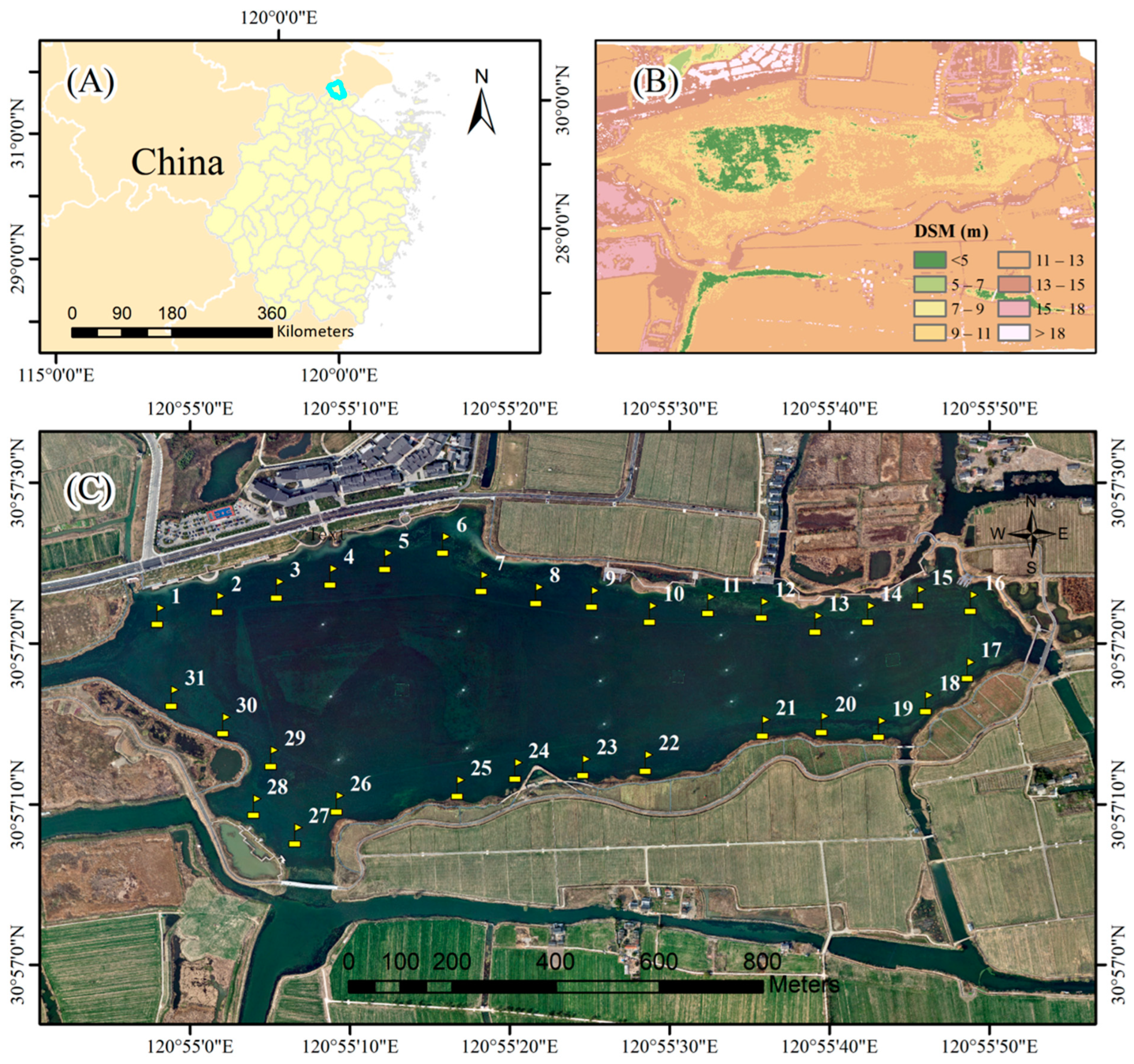
2.1. Study Area

Xiangfudang Wetland Park is a typical rural wetland in the Yangtze River Delta region, with center geographical coordinates of 30°57′17″ N latitude and 120°55′20″ E longitude (Figure 1A). The study area is approximately cover 180 ha2, of which the central lake area of the wetland is about 62 ha2 in size, with an average water depth of 7.5 m. The average annual temperature in the region is 15.4~16.4 °C; the number of hours of sunshine per year for 2007~2179 h. The average annual precipitation is close to 2000 mm, but the distribution is uneven, with rain concentrated from May to June. In general, the climate is mild and humid with abundant rainfall, which is typical of a subtropical monsoon climate, with flat terrain, rich species, and favorable ecological conditions.

2.2. Data Collection

2.2.1. In Situ Water Quality Parameters Data Collection

On June 15 (summer day) and November 26 (winter day) of 2023, two water quality surveys were conducted at Xiangfudang Wetland Park. The sampling periods were strategically chosen to correspond with the wet and dry seasons in the study area. Then, a total of 62 water quality sampling points were established, with 31 samples collected in June and another 31 in November. Based on satellite remote sensing images, 35 sampling points were initially evenly distributed, with the straight-line distance between neighboring sampling points greater than 100 m. After the field investigation, the points interfered by vegetation and other environmental factors were excluded, a total of 31 sample points were retained and set up, and their spatial distribution is shown in Figure 1C.
At each sampling point, 200 mL of water was taken at a depth of 50 cm below the water surface using a specialized water sampler, and water quality was then analyzed in the laboratory. The water quality parameters included TN [44], TP [45], COD [46], and TUB [47]. The detection of TN and TP employed the spectrophotometry method, utilizing the absorbance at specific wavelengths to determine the concentrations of nitrogen and phosphorus in the water samples. The determination of COD were carried out using the permanganate oxidation method. This method employed potassium permanganate as an oxidizing agent to digest the residues in the solution under neutral pH conditions. TUB was measured using the nephelometric method to assess the turbidity of suspended and colloidal particles in water. The TUB detection instrument used was the TU5200 benchtop turbidimeter, and the unit of measurement for the results is expressed in Nephelometric Turbidity Units (NTU).

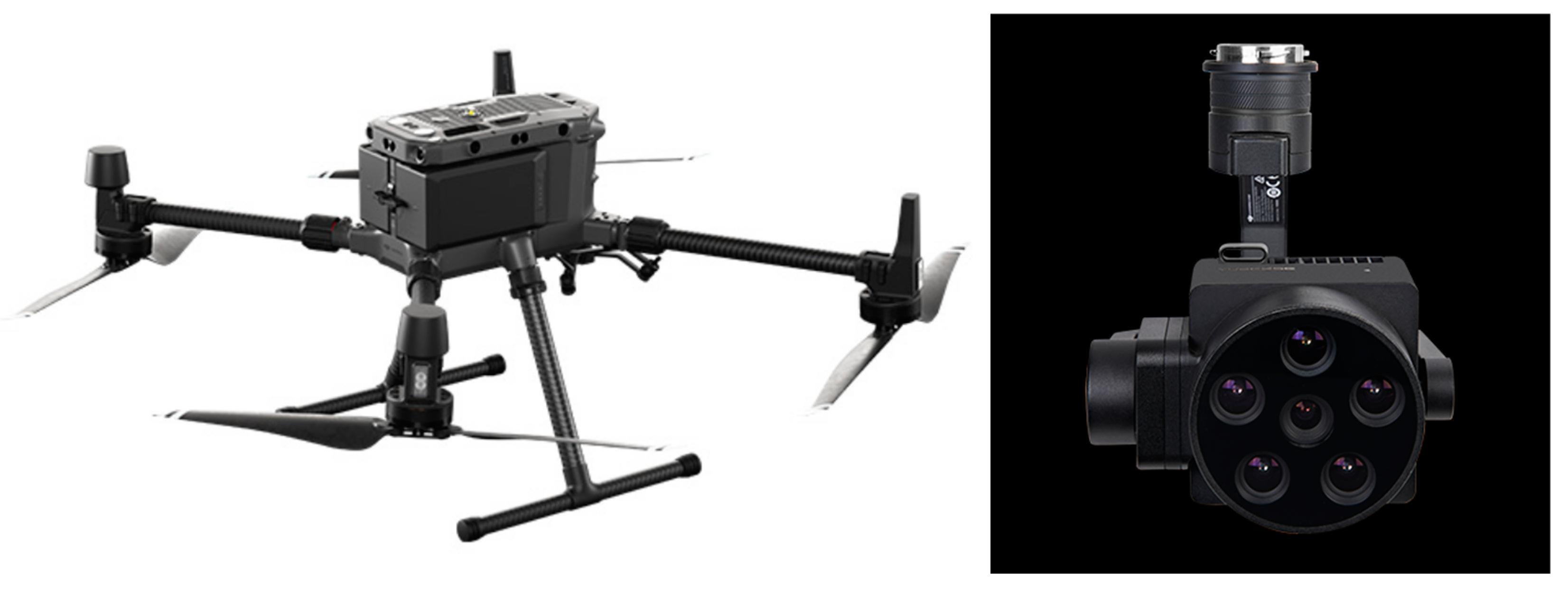
2.2.2. Drone Aerial Imagery Data Collection

In this study, a DJI Matrice300 RTK UAV (DJI, Shenzhen, Guangdong, China) equipped with a Changguang Yuchen AQ600 Pro multispectral camera (YUSENSE Information Technology and Equipment (Qingdao) Co., Ltd., Qingdao City, Shandong Province, China) was used to acquire high-resolution images (Figure 2). The Changguang Yuchen AQ600 Pro has five 3.2 M-pixel multispectral CMOS sensors, collects reflectance information in the following five narrow wavelength bands (Table 1), and has one 12.3 M-pixel color sensor, acquire full-color RGB images. The drone aerial photography and water quality field sampling were conducted simultaneously. The flight altitude of the UVA was set at 200 m, and the flight speed was 8 m/s. To facilitate data splicing in the later stage, the overlap degree of the heading was set at 60%, and the overlap degree of the side direction was set at 70%. Ultimately, a total of four flight paths were completed over two aerial surveys, yielding 3304 × 6 RAW images of the study area, with a spatial resolution of 8.8 cm.
After completing the drone flight operations, Yusense Map software, version 2.2.5 (Changguang Yuchen company, Qingdao City, Shandong Province, China) was used for image stitching and geometric correction, as well as radiometric correction. Then, considering that individual pixels are easily affected by specular reflection and water splashing, it was difficult to reflect the spectral differences caused by actual changes in water quality at the sampling sites [48]. We normalized the DN values for each band based on the following equation.
Spectral Response = (DN − DNmin)/(DNmax − DNmin)
where DN represents the digital number of each pixel, and the DNmin means the minimum DN of the band; similarly, the DNmax represents the maximum DN of the band. The standardized spectral response values were between 0 and 1. After normalizing the band data, mean filtering was applied to further mitigate the impact of speckle noise in the images. Finally, the water body regions were extracted for subsequent water quality estimation.

2.3. Water Quality Parameters Estimation

The objective of this study was the inversion and change analysis of water quality parameters using UAV aerial images and water quality ground sampling data; the specific technical route is shown in Figure 3. First, based on drone aerial imagery, the water bodies in the study area were extracted by the image segmentation algorithm. And then, combining the water quality sampling measured data and the corresponding visible and multispectral images taken by UAV aerial photography, machine learning algorithms were used to construct the model for water quality parameters’ estimation. Finally, the optimal modeling method was selected to realize water quality parameters mapping in the study area.

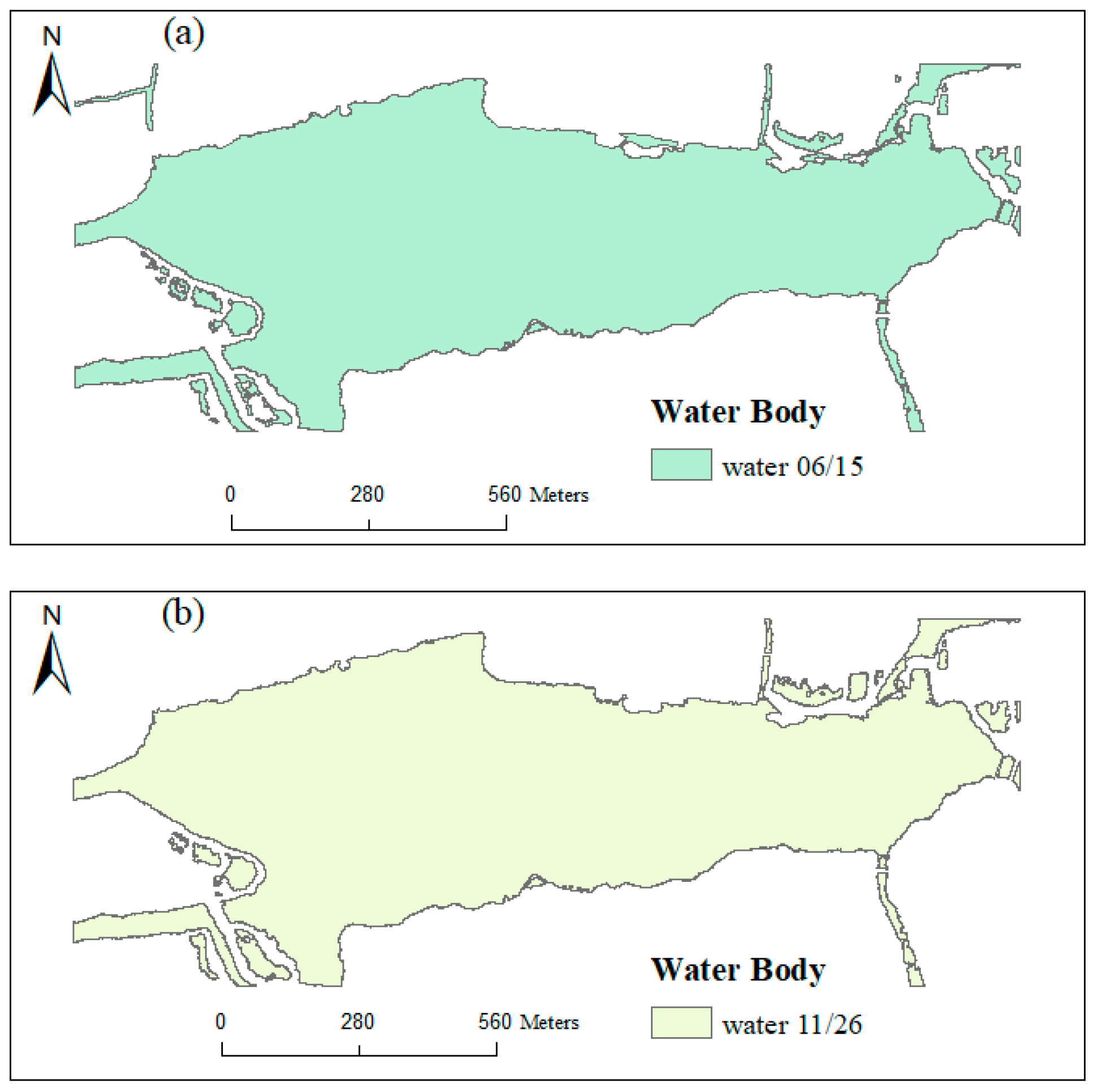
2.3.1. Extracted Water Body Area

Based on panchromatic RGB image, image segmentation was performed by the simple linear iterative clustering (SLIC) algorithm. The SLIC is a hyperpixel segmentation algorithm that efficiently generates hyperpixels by an iterative clustering method, with better boundary adhesion, speed, memory efficiency, and improves segmentation performance [49]. Then, water body patches were merged using visual discrimination to obtain 2 periods of complete vector data of water bodies within the study area. Based on the UAV image analysis, the extracted spatial distribution of waters in summer (15 June) and winter (26 November) in 2023 is shown in Figure 4. The statistical results show that the watershed area was about 69.54 hm2 in summer and 66.29 hm2 in winter. The change of water body area mainly occurred in the western part of the study area, as well as in the northeastern region, where the main body of water extended to the edge of the surrounding wetlands.

2.3.2. Feature Variable Dataset Construction and Feature Selection

In water quality remote sensing, typical spectral indices often involve dual-band combinations. Compared to single-band modeling, dual-band combinations can mitigate noise interference and emphasize the spectral characteristics of water quality parameters, thereby enhancing the accuracy of water quality inversion models [50]. In this study, we utilized summation, subtraction, and ratio operations on any two or three out of five single spectral bands to construct a dataset of 51 features as candidate predictor variables (Table 2).
In this study, the Recursive Feature Elimination (RFE) algorithm was employed for feature selection. Utilizing a Random Forest model, Recursive Feature Elimination with Cross-Validation (RFECV) was applied to determine feature importance [51]. Then, the top six feature variables were selected based on their importance ranking. This method ensures that the most significant features are retained, enhancing the model’s predictive performance while reducing overfitting and improving interpretability.

2.3.3. Machine Learning Methods

Based on the experience of related research, four ML algorithms, including Random Forest (RF), Support Vector Regression (SVR), Post-feedback neural network (ANN), and CatBoost regression, were employed to build estimation models for each target variable (TN, TP, COD and TUB). All of them are common models that have performed relatively well in previous research [42,52,53]. We employed a systematic hyperparameter tuning process using a grid search [15] to identify the optimal settings for each algorithm. Meanwhile, considering the limited sample data on which the model relies, we preferred to simplify the model structure and tried our best to avoid overfitting when setting the model parameters.
RF is an ML algorithm based on decision trees that was developed by Breiman in 2001 [54]. It operates by constructing a multitude of decision trees during training and outputting the mean prediction (regression) or the mode of the predictions (classification) of the individual trees [55]. RF is known for its robustness and ability to handle large datasets with high dimensional, making it a popular choice across various machine learning applications. In this study, the RF model construction was based on the sklearn.ensemble package for Python, and the chosen parameters were n_estimators (800), min_sample_split (2), min_sample_leaf (1), max_features (auto), and max_depth (50) for the RF model used for water quality parameters’ estimation.
Support Vector Regression (SVR) is a supervised learning algorithm used for regression tasks. It works by finding a hyperplane in a high-dimensional space that best fits the training data [56]. The objective is to minimize the error between the predicted and actual values while maximizing the margin, which is the distance between the hyperplane and the closest data points. SVR is effective for handling non-linear relationships in data through the use of kernel functions, allowing it to capture complex patterns and achieve robust regression performance [57]. The regularization parameter (C = 1.0), kernel type (default = ‘rbf’), and epsilon (epsilon = 0.1).
ANN is a type of neural network algorithm [58]. It iteratively adjusts weights based on prediction errors, making it effective for modeling complex relationships in data for tasks like regression and classification. The BP involves input, hidden, and output layers and operates in two main stages: forward propagation and error back-propagation [15]. During back-propagation, errors are propagated from the output layer back through the hidden layers, adjusting the weights iteratively across all units in each layer. This process continues until the error is minimized to an acceptable level through repeated training. The number of features selected determines the number of input nodes of the BP model. The input variables used in this study were 5 dimensional, and after testing and improving different hidden layer structures, the final ANN model used had 4 hidden layers, and the number of nodes was 64–32–16–4, with learning rate (0.01) and activation functions (ReLU).
CatBoost regression is a gradient boosting algorithm designed to handle categorical features effectively [59]. It sequentially builds an ensemble of trees where each subsequent tree corrects errors made by the previous ones, enhancing the model’s predictive power. It utilizes efficient methods to convert categorical features into numerical values during training and incorporates regularization techniques such as learning rate shrinkage and feature importance computation to prevent over fitting [60]. The CatBoost regression model in this study was constructed based on the “CatBoost” package for Python. The chose parameters were n_estimators (600), learning_rate (0.01), eval_metric (RMSE), and max_depth (4) for the CatBoost model in this study.

2.3.4. Accuracy Evaluation

During the model construction process, 70% of the data with a certain concentration gradient were chosen for the training dataset, 15% were chosen for the validation dataset, and 15% were chose for the testing. The performance of the models was assessed based on the coefficient of determination (R2), and Root Mean Square Error (RMSE). The default assumption for the model’s errors is that they follow an independent normal distribution. The formulas for various error evaluation metrics are as follows:
R 2 = 1 y _ t r u e y _ p r e d 2 / y _ t r u e y _ m e a n 2
R M S E = 1 / n × y _ p r e d y _ t r u e
where y_true represents the measured value of the water quality parameters, y_pred represents the predicted values of the water quality parameters, and n is the number of the sampling points.

2.3.5. Spatiotemporal Analysis of Water Quality in Xiangfudang

The machine learning model with the best validation results was selected and inputted into the raster feature data of the UAV to realize the estimation of water quality parameters at the regional scale. Afterward, based on the environmental quality standards for surface water in China [13] and Quality Standard of Reclaimed Water [61] (Table 3), we analyzed the water quality characteristics of the Xiangfudang region and its seasonal changes through spatial and temporal statistics.

3. Results

3.1. Data Overview

Table 4 lists the statistical values of the TP, TN, COD, and TUB, along with their corresponding data in the five bands (Blue, Green, Red, Edge_red, and NIR) of the UAV multispectral data. The dataset was analyzed using the maximum, minimum, mean, standard deviation, 25% quantile, 50% quantile, and 75% quantile. A total of 62 sample points, the average value of the TN was 1.19 ± 0.83 gm/L, TP was 0.14 ± 0.07 gm/L, COD was 9.10 ± 6.98 gm/L, and TUB was 17.76 ± 5.83 NTU, which were all within the nationally defined safety limits according to China’s water quality testing standards.
The statistical information of water quality measurements data for the two sampling periods (15 June and 26 November 2023 are shown in Figure 5. Most of the four water quality parameters (TN, TP, COD, and TUB) are show non-normal distributions. The comparison of parameter characteristics between the two periods reveals that the most significant difference was observed in COD, which were higher in summer (11.14 mg/L) compared to winter (6.97 mg/L). The average TN concentration in both summer and autumn was approximately 1 mg/L, while the TP concentration was around 0.1 mg/L. The average TUB for both seasons was 17 UNT.

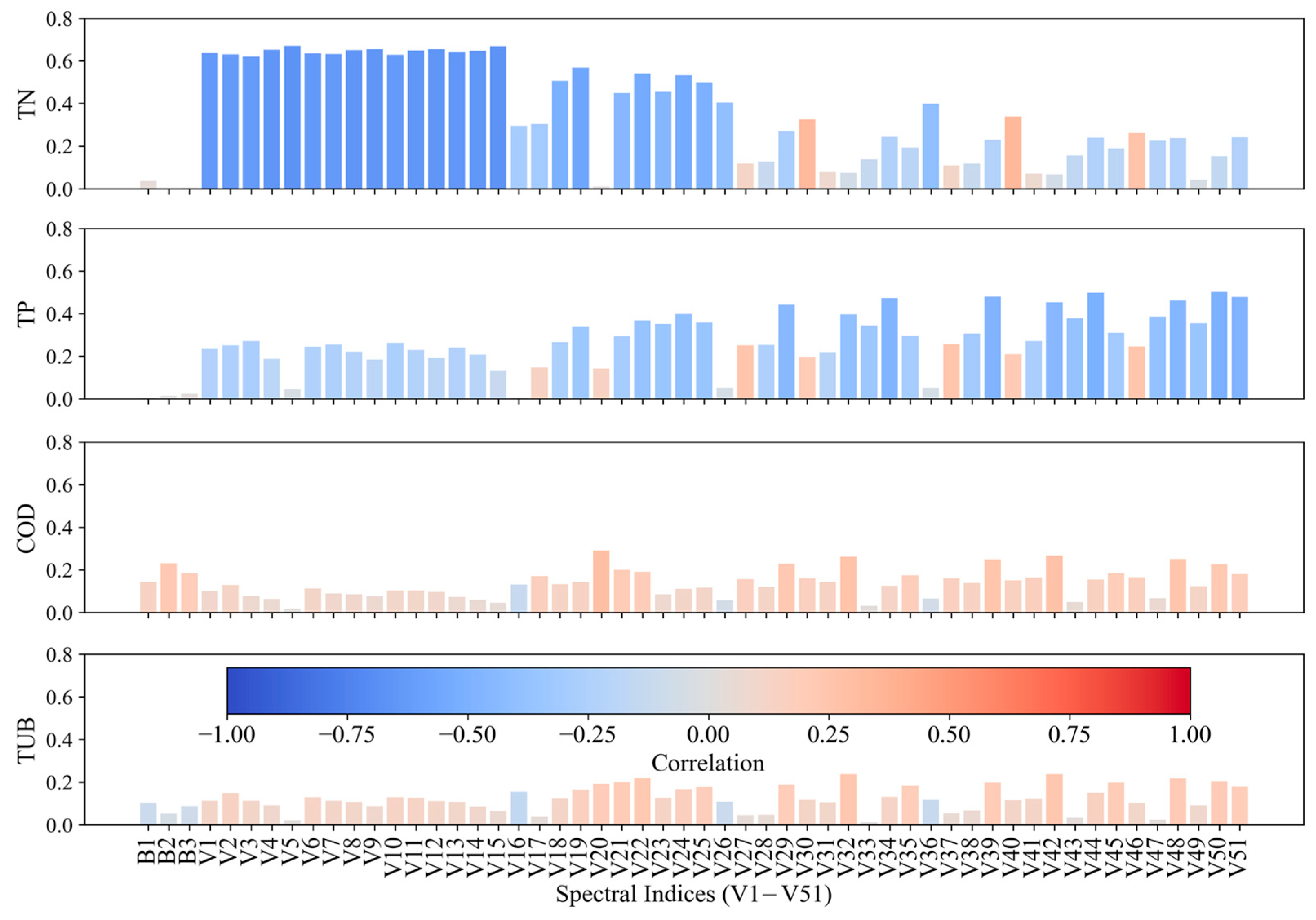
3.2. Spectral Index and Water Quality Parameters’ Correlation Analysis

Pearson correlation analysis was used to identify the most relevant features in the water quality parameters and spectral indices. Figure 6 presents the magnitude of the correlation between the three panchromatic image bands (R, G, B), the 51 spectral characteristic indices, and each of the water quality parameters. Among the four water parameters, TN had the highest correlation coefficients with spectra indices, where the highest correlated spectral index was V5 (NIR) with a −0.64 correlation values. V44 ((red − NIR)/(red + NIR)) was the most correlated spectral index for TP, with a value of −0.47, and V20 (green − red) was the most correlated spectral index for COD (with a values of 0.26). The TN and TP concentrations were correlated negatively with most of the spectral indices, while both COD and TUB and most of the spectral values showed weak positively correlation. Compared to TN and TP, the three panchromatic image bands (RGB) showed higher correlations with COD and TUB, indicating that panchromatic images may be less suitable for estimating TN and TP concentrations.

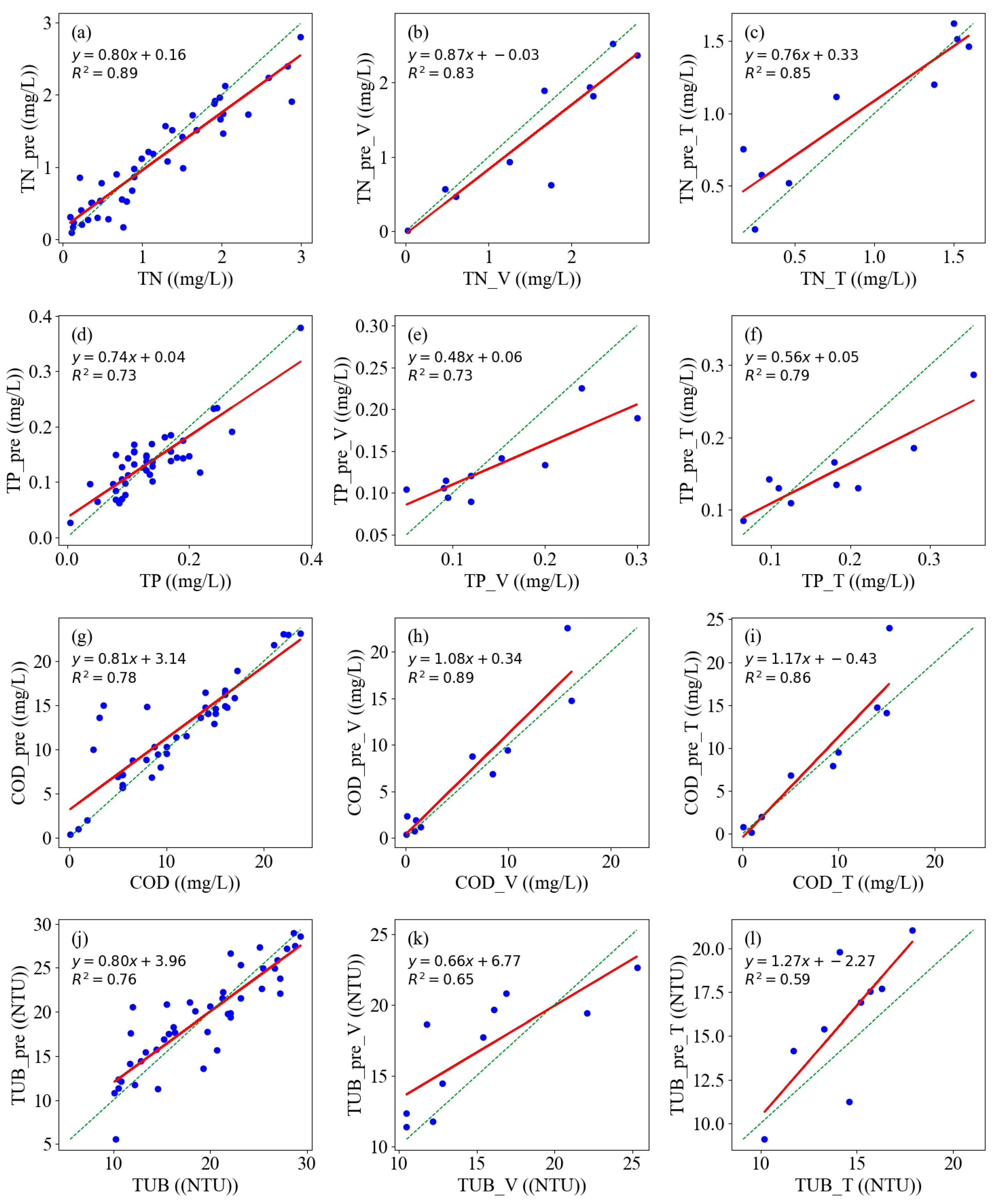
3.3. The Performance of Estimation Models

Utilizing the Recursive Feature Elimination with Cross-Validation (RFECV) model, the selected feature variables for TN were identified as V4 (Edge_red), V5 (NIR), V11 (green + Edge_red), V15 (green + NIR), and V48 ((blue + Edge_red − NIR)/(blue + Edge_red + NIR)). For TP, the selected features are V29 (blue/NIR), V32 (green/NIR), V44 ((red − NIR)/(red + NIR)), V50 ((green + red − NIR)/(green + red + NIR)), and V51 ((red + Edge_red − NIR)/(red + Edge_red + NIR)). In the case of COD, the variables B2 (G), V20 (green − red), V32 (green/NIR), V39 ((blue − NIR)/(blue + NIR), and V42 ((green − NIR)/(green + NIR)) were determined to be significant. Meanwhile, for TUB, the relevant features were V2 (green), V6 (blue + green), V28 (blue/Edge_red), V32 (green/NIR), and V42 ((green − NIR)/(green + NIR)). Using the selected variables, models were constructed with 70% of the data allocated for training and the remaining 30% reserved for validation. Four distinct machine learning algorithms were employed to build these models. The specific performance metrics and outcomes of these models are detailed in Table 5.
Overall, the models achieved satisfactory performance, with the R2 values for the models of all four water quality parameters exceeding 0.6 (Figure 7). Notably, the models constructed using the ANN algorithm yielded the best results for estimating TN, COD, and TUB; the R2 values of the model validation (Testing) were 0.83 (0.85) (Figure 7b,c), 0.89 (0.86) (Figure 7h,i), and 0.65 (0.59) (Figure 7k,l), respectively. Conversely, the CatBoost algorithm demonstrated superior performance in estimating TP, with validation R2 and RMSE values of 0.73 and 0.02 mg/L (Figure 7e), and Testing R2 and RMSE values of 0.79 and 0.03 mg/L (Figure 7f).

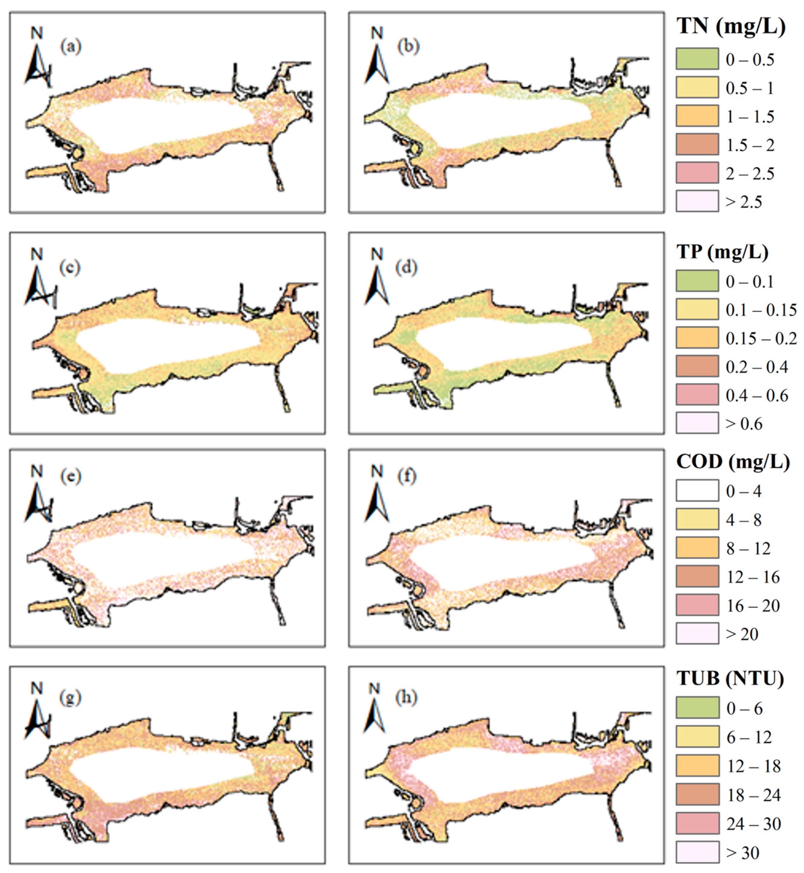
3.4. Water Quality Parameters’ Inversion by UAV Images

Figure 8 shows the regional estimation results of the four water quality parameters in two periods, including the TN (Figure 8a,b), TP (Figure 8c,d), COD (Figure 8e,f), and TUB (Figure 8g,h). In terms of spatial patterns, none of the four water quality metrics showed significant variability between the summer (15 June) and winter (26 November) periods. The spatial results were analyzed only for the area surrounding the sample, taking into account the errors caused by specular reflections from the water column. The mean TN concentration was 1.34 mg/L during the summer, with a variance of 0.86, and 1.16 mg/L during the winter (variance of 0.75). For TP, the mean concentrations were 0.16 ± 0.06 mg/L in the summer and 0.14 ± 0.07 mg/L in the winter. Similar to the site survey data, the COD was slightly higher in summer than in winter, with values of 16.05 ± 9.87 mg/L and 13.02 ± 8.22 mg/L, respectively. The mean TUB in the summer was 18.39 NTU with a variance of 7.23 NTU, while in the winter, the mean was 20.03 NTU with a variance of 7.52 NUT.

4. Discussion

4.1. Water Quality Monitoring Based on UAV Images

In the traditional wetland monitoring index survey, only the actual laboratory measurements of water samples actually obtained are the most accurate, but it requires a lot of human and material resources and financial resources, is confined to the range of sample points, and the estimation of water quality indexes at the non-sample points is more subjective and with larger errors [62,63]. The remote sensing image looks down on the overall structure of the wetland from above, and the spliced and reconstructed data can reflect the spectral information of the waters well [35,64,65]. The inverse monitoring of wetland water quality using intermediate products generated from remote sensing image data was significantly better than the field sampling and detection methods, both in terms of efficiency and accuracy.
Both the current experiment and previous studies have demonstrated that UAVs are indeed suitable systems for monitoring water bodies and water quality. The near-ground remote sensing data obtained through UAVs can effectively estimate water quality parameters [29,66,67]. The water quality parameters examined in this study, including TN, TP, COD, and TUB, RGB three bands of panchromatic images, and spectral indices constructed from five multispectral bands (blue, green, red, Edge_red, and NIR), were used as candidate feature variables. Both the correlation analysis between the candidate independent variables and the four water quality parameters, as well as the feature selection based on the RFECV algorithm, indicated that multispectral data better reflected water quality conditions, particularly the Edge_red and NIR bands (Figure 6 and Table 4). Multispectral sensors are more costly than panchromatic image sensors but are also really more suitable for water quality monitoring [15,26,68].
The superior performance of Edge_red and NIR bands in the inversion of water quality parameters may be the greater light penetration of these bands compared to visible light (blue, red and green), which allows for the detection of deeper information about the water body [69]. As a result, these bands were able to capture the overall condition of the water body, including potential water quality problems. Meanwhile, the Edge_red (690–750 nm) and NIR (750–2500 nm) are very sensitive to the reflectance of plant leaves and algae [70]. The concentration and distribution of phytoplankton (e.g., algae) in the water column tends to influence water quality parameters, such as chlorophyll content, as well as suspended and organic matter content [71]. The Edge_red and NIR bands can more accurately capture changes in the biosignatures of these plants [72], thus providing more effective water quality estimates.
However, the comparative analysis of the inversion results from two different periods revealed that environmental factors could introduce errors in water quality monitoring. Although this study employed normalized filtering to minimize salt-and-pepper noise in water body area, some uncertainty persisted in the spatial estimation results. Subsequently, methods such as data class analysis can be considered to reduce the impact of salt-and-pepper noise [73]. Meanwhile, it is recommended to conduct aerial surveys under similar climatic conditions and preferably in the late afternoon to reduce the effects of specular reflection [74]. Additionally, higher-frequency data collection using UAV imagery is advised to mitigate the uncertainties in result comparisons caused by environmental and other influencing factors.

4.2. Water Quality Monitoring in Xiangfudang Wetland Park

In order to promote the integrated development of the Yangtze River Delta (YRD) region, the Yangtze River Delta Eco-Green Integration Demonstration Zone was formally approved and established on October 25, 2019, by China’s State Council. The demonstration zone emphasizes green and ecological development, and its ecological environment, air quality, and water quality conditions have been given key attention. Ying et al. [29] tested and analyzed the water quality of Qingshan Lake, which is also in the Yangtze River Delta region, and showed that its suspended solids was 30.21 (mg/L), and the average value of TUB was 18.07 UNT. Lu et al. [75] analyzed the quality of rural cited water in the Yangtze River Delta region during the abundant (summer) and dry (winter) periods, showing that TP was about 0.149 mg/L during the abundant period and 0.047 mg/L during the dry period, and TN was 0.344 mg/L during the abundant period and 0.208 mg/L during the dry period.
Based on our investigations, the water quality of the water bodies in the Xiangfudang area after the 2019 retrofit project has generally conformed to the surface water quality requirements [11]. Comparison of water quality parameters between summer and winter showed that TN, TP, and COD were slightly higher in summer than in winter (Figure 8). Summer is usually accompanied by frequent rainfall, and especially when the intensity of rainfall is high, surface runoff will carry nitrogen and phosphorus carried by soil, agricultural fertilizers, and livestock and poultry excreta into the water body [76]. This process significantly increases the TN and TP loads in the water body, while the organic matter carried in the runoff also elevates COD levels. In addition, abundant sunlight and warmer water temperatures in summer favor the rapid growth and reproduction of phytoplankton and algae [77]. These plants absorb nitrogen and phosphorus from the water during their growth and release them back into the water after their death and decomposition, further increasing the concentrations of TN and TP [78]. Meanwhile, the overpopulation of algae may trigger eutrophication of the water body, which increases the content of organic matter, thus elevating the COD value. However, the lower TUB in summer compared to winter may be due to the fact that more people come to the wetland park in summer for recreation and cooling, and more frequent water cleaning is conducted manually.
For this water quality monitoring study in the Xiangfudang Wetland Park, we also interviewed people in the neighborhood during the water quality sampling period. After the water body project renovation, the community had strengthened the management of the wetland park, not only the water quality of the water body but also the surrounding vegetation and ecological communities. By transforming the environment, it really enhanced the well-being of the people living in the neighborhood. At the same time, the beautiful environment radiated the surrounding, attracting more tourists and bringing the community economic enhancement. Local residents also had more motivation and awareness to protect the water quality of the region, and this virtuous cycle will become the support of regional ecological sustainable development [79].

5. Conclusions

The objective of this study was to achieve water quality parameter (TN, TP, COD, and TUB) estimation based on UAV aerial images in the Xiangfudang Wetland Park. Combined sampling data from water quality monitoring stations and UAV images of two periods in 2023 and four machine learning algorithms were employed to construct parameter estimation models. ANN performed best for TN, COD, and TUB, with validation R2 values of 0.78, 0.76, and 0.57, respectively, while CatBoost yielded the highest accuracy for TP estimation (R2 = 0.72, RMSE = 0.05 mg/L). The red edge and near-infrared bands were most effective for water quality monitoring. Spatial results showed average TN concentrations of 1.34 mg/L (summer) and 1.16 mg/L (winter), while TP levels were 0.16 ± 0.06 mg/L (summer) and 0.14 ± 0.07 mg/L (winter). COD was higher in summer (16.05 ± 9.87 mg/L) compared to winter (13.02 ± 8.22 mg/L), with TUB at 18.39 NTU (summer) and 20.03 NTU (winter). The water quality met surface water standards, with slight seasonal variations. Our findings highlight the value of UAV-based multispectral imagery for efficient rural wetland water quality monitoring and recommend higher-frequency data collection to reduce uncertainties due to environmental factors.

Author Contributions

Conceptualization, N.Z. and Y.W.; methodology, H.Z.; software, N.Z. and S.D.; validation, L.M., Y.Z. and Z.H.; data curation, H.Z.; writing—original draft preparation, L.M.; writing—review and editing, Y.W. All authors have read and agreed to the published version of the manuscript.

Funding

This research was funded by “PIONEER” and “LEADING GOOSE” R&D Program of Zhejiang, grant number No. 2022C02038; Key Laboratory of National Geographic Census and Monitoring, Ministry of Natural Resources, grant number of 2023NGCM10.

Data Availability Statement

Data are contained within the article.

Conflicts of Interest

The authors declare no conflicts of interest.

References

  1. Sharma, S.; Singh, P. Wetlands Conservation: Current Challenges and Future Strategies; John Wiley & Sons: Hoboken, NJ, USA, 2021. [Google Scholar]
  2. Cao, C.X.; Zhao, J.; Gong, P.; Ma, G.R.; Bao, D.M.; Tian, K.; Tian, R.; Niu, Z.G.; Zhang, H.; Xu, M.; et al. Wetland changes and droughts in southwestern China. Geomat. Nat. Hazards Risk 2012, 3, 79–95. [Google Scholar] [CrossRef]
  3. Li, Y.; Liu, F.; Zhang, C. Analysis of change trend of water environment and cause in the Dongting Lake wetland. Ecol. Environ. 2011, 20, 1295. [Google Scholar]
  4. Bhateria, R.; Jain, D. Water quality assessment of lake water: A review. Sustain. Water Resour. Manag. 2016, 2, 161–173. [Google Scholar] [CrossRef]
  5. Uddin, M.G.; Nash, S.; Rahman, A.; Olbert, A.I. A comprehensive method for improvement of water quality index (WQI) models for coastal water quality assessment. Water Res. 2022, 219, 118532. [Google Scholar] [CrossRef] [PubMed]
  6. Akhtar, N.; Syakir Ishak, M.I.; Bhawani, S.A.; Umar, K. Various Natural and Anthropogenic Factors Responsible for Water Quality Degradation: A Review. Water 2021, 13, 2660. [Google Scholar] [CrossRef]
  7. Verma, A.K.; Singh, T.N. Prediction of water quality from simple field parameters. Environ. Earth Sci. 2013, 69, 821–829. [Google Scholar] [CrossRef]
  8. Whigham, D.F.; Chitterling, C.; Palmer, B. Impacts of freshwater wetlands on water quality: A landscape perspective. Environ. Manag. 1988, 12, 663–671. [Google Scholar] [CrossRef]
  9. Pimparkar, A.M.; Patil, S.N.; Patil, B.D.; Kadam, A.K. Comparative assessment of wetland water quality from rural and urban area of Aurangabad District, Maharashtra, India using water quality index. HydroResearch 2023, 6, 269–278. [Google Scholar] [CrossRef]
  10. Pachepsky, Y.; Kierzewski, R.; Stocker, M.; Sellner, K.; Mulbry, W.; Lee, H.; Kim, M. Temporal Stability of Escherichia coli Concentrations in Waters of Two Irrigation Ponds in Maryland. Appl. Environ. Microbiol. 2018, 84, e01876-17. [Google Scholar] [CrossRef]
  11. Zhou, G.; Xu, J.; Hu, H.; Liu, Z.; Zhang, H.; Xu, C.; Zhou, X.; Yang, J.; Nong, X.; Song, B.; et al. Off-Axis Four-Reflection Optical Structure for Lightweight Single-Band Bathymetric LiDAR. IEEE Trans. Geosci. Remote Sens. 2023, 61, 1000917. [Google Scholar] [CrossRef]
  12. Zhou, G.; Tang, Y.; Zhang, W.; Liu, W.; Jiang, Y.; Gao, E.; Zhu, Q.; Bai, Y. Shadow Detection on High-Resolution Digital Orthophoto Map Using Semantic Matching. IEEE Trans. Geosci. Remote Sens. 2023, 61, 4504420. [Google Scholar] [CrossRef]
  13. State Environmental Protection Administration of China. GB 3838-2002. Environmental Quality Standards for Surface Water; Ministry of Environmental Protection of the People’s Republic of China: Beijing, China, 2002.
  14. Zhao, X.; Li, Y.; Chen, Y.; Qiao, X.; Qian, W. Water Chlorophyll a Estimation Using UAV-Based Multispectral Data and Machine Learning. Drones 2023, 7, 2. [Google Scholar] [CrossRef]
  15. Xiao, Y.; Guo, Y.; Yin, G.; Zhang, X.; Shi, Y.; Hao, F.; Fu, Y. UAV Multispectral Image-Based Urban River Water Quality Monitoring Using Stacked Ensemble Machine Learning Algorithms—A Case Study of the Zhanghe River, China. Remote Sens. 2022, 14, 3272. [Google Scholar] [CrossRef]
  16. Li, J.; Luo, G.; He, L.; Xu, J.; Lyu, J. Analytical Approaches for Determining Chemical Oxygen Demand in Water Bodies: A Review. Crit. Rev. Anal. Chem. 2018, 48, 47–65. [Google Scholar] [CrossRef]
  17. Anh, N.T.; Can, L.D.; Nhan, N.T.; Schmalz, B.; Luu, T.L. Influences of key factors on river water quality in urban and rural areas: A review. Case Stud. Chem. Environ. Eng. 2023, 8, 100424. [Google Scholar] [CrossRef]
  18. Behmel, S.; Damour, M.; Ludwig, R.; Rodriguez, M.J. Water quality monitoring strategies—A review and future perspectives. Sci. Total Environ. 2016, 571, 1312–1329. [Google Scholar] [CrossRef]
  19. Chebud, Y.; Naja, G.M.; Rivero, R.G.; Melesse, A.M. Water Quality Monitoring Using Remote Sensing and an Artificial Neural Network. Water Air Soil Pollut. 2012, 223, 4875–4887. [Google Scholar] [CrossRef]
  20. Yang, H.; Kong, J.; Hu, H.; Du, Y.; Gao, M.; Chen, F. A Review of Remote Sensing for Water Quality Retrieval: Progress and Challenges. Remote Sens. 2022, 14, 1770. [Google Scholar] [CrossRef]
  21. Sun, X.; Zhang, Y.; Shi, K.; Zhang, Y.; Li, N.; Wang, W.; Huang, X.; Qin, B. Monitoring water quality using proximal remote sensing technology. Sci. Total Environ. 2022, 803, 149805. [Google Scholar] [CrossRef]
  22. Jiang, Y.; Kong, J.; Zhong, Y.; Zhang, J.; Zheng, Z.; Wang, L.; Liu, D. The optimal method for water quality parameters retrieval of urban river based on machine learning algorithms using remote sensing images. Int. J. Remote Sens. 2023, 45, 7297–7317. [Google Scholar] [CrossRef]
  23. Zeng, N.; He, H.; Ren, X.; Zhang, L.; Zeng, Y.; Fan, J.; Li, Y.; Niu, Z.; Zhu, X.; Chang, Q. The utility of fusing multi-sensor data spatio-temporally in estimating grassland aboveground biomass in the three-river headwaters region of China. Int. J. Remote Sens. 2020, 41, 7068–7089. [Google Scholar] [CrossRef]
  24. Sagan, V.; Peterson, K.T.; Maimaitijiang, M.; Sidike, P.; Sloan, J.; Greeling, B.A.; Maalouf, S.; Adams, C. Monitoring inland water quality using remote sensing: Potential and limitations of spectral indices, bio-optical simulations, machine learning, and cloud computing. Earth-Sci. Rev. 2020, 205, 103187. [Google Scholar] [CrossRef]
  25. Qin, H.; Zhou, W.; Yao, Y.; Wang, W. Individual tree segmentation and tree species classification in subtropical broadleaf forests using UAV-based LiDAR, hyperspectral, and ultrahigh-resolution RGB data. Remote Sens. Environ. 2022, 280, 113143. [Google Scholar] [CrossRef]
  26. Chen, B.; Mu, X.; Chen, P.; Wang, B.; Choi, J.; Park, H.; Xu, S.; Wu, Y.; Yang, H. Machine learning-based inversion of water quality parameters in typical reach of the urban river by UAV multispectral data. Ecol. Indic. 2021, 133, 108434. [Google Scholar] [CrossRef]
  27. Lu, Q.; Si, W.; Wei, L.; Li, Z.; Xia, Z.; Ye, S.; Xia, Y. Retrieval of Water Quality from UAV-Borne Hyperspectral Imagery: A Comparative Study of Machine Learning Algorithms. Remote Sens. 2021, 13, 3928. [Google Scholar] [CrossRef]
  28. Arroyo-Mora, J.P.; Kalacska, M.; Løke, T.; Schläpfer, D.; Coops, N.C.; Lucanus, O.; Leblanc, G. Assessing the impact of illumination on UAV pushbroom hyperspectral imagery collected under various cloud cover conditions. Remote Sens. Environ. 2021, 258, 112396. [Google Scholar] [CrossRef]
  29. Ying, H.; Xia, K.; Huang, X.; Feng, H.; Yang, Y.; Du, X.; Huang, L. Evaluation of water quality based on UAV images and the IMP-MPP algorithm. Ecol. Inform. 2021, 61, 101239. [Google Scholar] [CrossRef]
  30. Kageyama, Y.; Takahashi, J.; Nishida, M.; Kobori, B.; Nagamoto, D. Analysis of water quality in Miharu dam reservoir, Japan, using UAV data. IEEJ Trans. Electr. Electron. Eng. 2016, 11, S183–S185. [Google Scholar] [CrossRef]
  31. Su, T.-C. A study of a matching pixel by pixel (MPP) algorithm to establish an empirical model of water quality mapping, as based on unmanned aerial vehicle (UAV) images. Int. J. Appl. Earth Obs. Geoinf. 2017, 58, 213–224. [Google Scholar] [CrossRef]
  32. Zeng, C.; Richardson, M.; King, D.J. The impacts of environmental variables on water reflectance measured using a lightweight unmanned aerial vehicle (UAV)-based spectrometer system. ISPRS J. Photogramm. Remote Sens. 2017, 130, 217–230. [Google Scholar] [CrossRef]
  33. Zhang, R.; Wang, Z.; Li, X.; She, Z.; Wang, B. Water Quality Sampling and Multi-Parameter Monitoring System Based on Multi-Rotor UAV Implementation. Water 2023, 15, 2129. [Google Scholar] [CrossRef]
  34. Hou, Y.; Zhang, A.; Lv, R.; Zhang, Y.; Ma, J.; Li, T. Machine learning algorithm inversion experiment and pollution analysis of water quality parameters in urban small and medium-sized rivers based on UAV multispectral data. Environ. Sci. Pollut. Res. 2023, 30, 78913–78932. [Google Scholar] [CrossRef] [PubMed]
  35. Liu, Y.; Xia, K.; Feng, H.; Fang, Y. Inversion of water quality elements in small and micro-size water region using multispectral image by UAV. Acta Sci. Circumstantiae 2019, 39, 1241–1249. [Google Scholar]
  36. Lo, Y.; Fu, L.; Lu, T.; Huang, H.; Kong, L.; Xu, Y.; Zhang, C. Medium-Sized Lake Water Quality Parameters Retrieval Using Multispectral UAV Image and Machine Learning Algorithms: A Case Study of the Yuandang Lake, China. Drones 2023, 7, 244. [Google Scholar] [CrossRef]
  37. Kwon, Y.S.; Pyo, J.; Kwon, Y.-H.; Duan, H.; Cho, K.H.; Park, Y. Drone-based hyperspectral remote sensing of cyanobacteria using vertical cumulative pigment concentration in a deep reservoir. Remote Sens. Environ. 2020, 236, 111517. [Google Scholar] [CrossRef]
  38. Altenburger, R.; Ait-Aissa, S.; Antczak, P.; Backhaus, T.; Barceló, D.; Seiler, T.-B.; Brion, F.; Busch, W.; Chipman, K.; de Alda, M.L.; et al. Future water quality monitoring—Adapting tools to deal with mixtures of pollutants in water resource management. Sci. Total Environ. 2015, 512–513, 540–551. [Google Scholar] [CrossRef] [PubMed]
  39. Irie, M.; Manabe, Y.; Yamashita, M. Estimation Method of Chlorophyll Concentration Distribution Based on UAV Aerial Images Considering Turbid Water Distribution in a Reservoir. Drones 2024, 8, 224. [Google Scholar] [CrossRef]
  40. Zeng, N.; Ren, X.; He, H.; Zhang, L.; Li, P.; Niu, Z. Estimating the grassland aboveground biomass in the Three-River Headwater Region of China using machine learning and Bayesian model averaging. Environ. Res. Lett. 2021, 16, 114020. [Google Scholar] [CrossRef]
  41. Zeng, N.; Ren, X.; He, H.; Zhang, L.; Zhao, D.; Ge, R.; Li, P.; Niu, Z. Estimating grassland aboveground biomass on the Tibetan Plateau using a random forest algorithm. Ecol. Indic. 2019, 102, 479–487. [Google Scholar] [CrossRef]
  42. Zhu, M.; Wang, J.; Yang, X.; Zhang, Y.; Zhang, L.; Ren, H.; Wu, B.; Ye, L. A review of the application of machine learning in water quality evaluation. Eco-Environ. Health 2022, 1, 107–116. [Google Scholar] [CrossRef]
  43. Fan, Z. Research of Low-Carbon Urban Area Planning for Carbon Peaking and Carbon Neutrality Goals—A Case Study of XiangFu Dang District in Jianshan. Master’s Thesis, Beijing University of Civil Engineering and Architecture, Beijing, China, 2023. [Google Scholar]
  44. Ministry of Environmental Protection of China. GB 11894-89. Water Quality-Determination of Total Nitrogen-Alkaline Potassium Persulfate Digestion-UV Spectrophotometric Method; China Standard Press: Beijing, China, 1989.
  45. Ministry of Environmental Protection of China. GB 11893-89. Water Quality-Determination of Total Phosphorus-Ammonium Molybdate Spectrophotometric Method; China Standard Press: Beijing, China, 1989.
  46. Ministry of Environmental Protection of China. GB 11914-89. Water Quality-Determination of Chemical Oxygen Demand-Dichromate Method; China Environmental Science Press: Beijing, China, 1989.
  47. Ministry of Environmental Protection of China. GB/T 13200. Water Quality-Determination of Turbidity-Nephelometric Method; China Standard Press: Beijing, China, 1994.
  48. Guo, Y.; Wang, H.; Wu, Z.; Wang, S.; Sun, H.; Senthilnath, J.; Wang, J.; Robin Bryant, C.; Fu, Y. Modified Red Blue Vegetation Index for Chlorophyll Estimation and Yield Prediction of Maize from Visible Images Captured by UAV. Sensors 2020, 20, 5055. [Google Scholar] [CrossRef] [PubMed]
  49. Achanta, R.; Shaji, A.; Smith, K.; Lucchi, A.; Fua, P.; Süsstrunk, S. SLIC Superpixels Compared to State-of-the-Art Superpixel Methods. IEEE Trans. Pattern Anal. Mach. Intell. 2012, 34, 2274–2282. [Google Scholar] [CrossRef]
  50. Wang, L.; Yue, X.; Wang, H.; Ling, K.; Liu, Y.; Wang, J.; Hong, J.; Pen, W.; Song, H. Dynamic Inversion of Inland Aquaculture Water Quality Based on UAVs-WSN Spectral Analysis. Remote Sens. 2020, 12, 402. [Google Scholar] [CrossRef]
  51. Awad, M.; Fraihat, S. Recursive Feature Elimination with Cross-Validation with Decision Tree: Feature Selection Method for Machine Learning-Based Intrusion Detection Systems. J. Sens. Actuator Netw. 2023, 12, 67. [Google Scholar] [CrossRef]
  52. Chiu, M.S.; Wang, J. Evaluation of Machine Learning Regression Techniques for Estimating Winter Wheat Biomass Using Biophysical, Biochemical, and UAV Multispectral Data. Drones 2024, 8, 287. [Google Scholar] [CrossRef]
  53. Haghiabi, A.H.; Nasrolahi, A.H.; Parsaie, A. Water quality prediction using machine learning methods. Water Qual. Res. J. 2018, 53, 3–13. [Google Scholar] [CrossRef]
  54. Breiman, L. Random Forests. Mach. Learn. 2001, 45, 5–32. [Google Scholar] [CrossRef]
  55. Park, J.; Kim, H.-C.; Bae, D.; Jo, Y.-H. Data Reconstruction for Remotely Sensed Chlorophyll-a Concentration in the Ross Sea Using Ensemble-Based Machine Learning. Remote Sens. 2020, 12, 1898. [Google Scholar] [CrossRef]
  56. Ding, S.; Zhang, N.; Zhang, X.; Wu, F. Twin support vector machine: Theory, algorithm and applications. Neural Comput. Appl. 2017, 28, 3119–3130. [Google Scholar] [CrossRef]
  57. Li, N.; Ning, Z.; Chen, M.; Wu, D.; Hao, C.; Zhang, D.; Bai, R.; Liu, H.; Chen, X.; Li, W.; et al. Satellite and Machine Learning Monitoring of Optically Inactive Water Quality Variability in a Tropical River. Remote Sens. 2022, 14, 5466. [Google Scholar] [CrossRef]
  58. Cockburn, J.; Holroyd, C.B. Feedback information and the reward positivity. Int. J. Psychophysiol. 2018, 132, 243–251. [Google Scholar] [CrossRef] [PubMed]
  59. Elith, J.; Leathwick, J.R.; Hastie, T. A working guide to boosted regression trees. J. Anim. Ecol. 2008, 77, 802–813. [Google Scholar] [CrossRef]
  60. Prokhorenkova, L.; Gusev, G.; Vorobev, A.; Dorogush, A.V.; Gulin, A. Catboost: Unbiased Boosting with Categorical Features. In Proceedings of the 32nd International Conference on Neural Information Processing Systems, Montréal, QC, Canada, 3–8 December 2018; pp. 6639–6649. [Google Scholar]
  61. Ministry of Water Resources of China. SL 368-2006. Water Quality Standard for Sewage Recycling; China Water & Power Press: Beijing, China, 2006.
  62. Horowitz, A.J. A Review of Selected Inorganic Surface Water Quality-Monitoring Practices: Are We Really Measuring What We Think, and If So, Are We Doing It Right? Environ. Sci. Technol. 2013, 47, 2471–2486. [Google Scholar] [CrossRef]
  63. Gray, M.J.; Chamberlain, M.J.; Buehler, D.A.; Sutton, W.B. Wetland Wildlife Monitoring and Assessment. In Wetland Techniques: Volume 2: Organisms; Anderson, J.T., Davis, C.A., Eds.; Springer: Dordrecht, The Netherlands, 2013; pp. 265–318. [Google Scholar]
  64. Adeli, S.; Salehi, B.; Mahdianpari, M.; Quackenbush, L.J.; Brisco, B.; Tamiminia, H.; Shaw, S. Wetland Monitoring Using SAR Data: A Meta-Analysis and Comprehensive Review. Remote Sens. 2020, 12, 2190. [Google Scholar] [CrossRef]
  65. Davranche, A.; Lefebvre, G.; Poulin, B. Wetland monitoring using classification trees and SPOT-5 seasonal time series. Remote Sens. Environ. 2010, 114, 552–562. [Google Scholar] [CrossRef]
  66. Matsui, K.; Shirai, H.; Kageyama, Y.; Yokoyama, H. Improving the resolution of UAV-based remote sensing data of water quality of Lake Hachiroko, Japan by neural networks. Ecol. Inform. 2021, 62, 101276. [Google Scholar] [CrossRef]
  67. Zhang, Y.; Jing, W.; Deng, Y.; Zhou, W.; Yang, J.; Li, Y.; Cai, Y.; Hu, Y.; Peng, X.; Lan, W.; et al. Water quality parameters retrieval of coastal mariculture ponds based on UAV multispectral remote sensing. Front. Environ. Sci. 2023, 11, 1079397. [Google Scholar] [CrossRef]
  68. Román, A.; Tovar-Sánchez, A.; Gauci, A.; Deidun, A.; Caballero, I.; Colica, E.; D’Amico, S.; Navarro, G. Water-Quality Monitoring with a UAV-Mounted Multispectral Camera in Coastal Waters. Remote Sens. 2023, 15, 237. [Google Scholar] [CrossRef]
  69. Timmer, B.; Reshitnyk, L.Y.; Hessing-Lewis, M.; Juanes, F.; Costa, M. Comparing the Use of Red-Edge and Near-Infrared Wavelength Ranges for Detecting Submerged Kelp Canopy. Remote Sens. 2022, 14, 2241. [Google Scholar] [CrossRef]
  70. Xie, Q.; Dash, J.; Huang, W.; Peng, D.; Qin, Q.; Mortimer, H.; Casa, R.; Pignatti, S.; Laneve, G.; Pascucci, S.; et al. Vegetation Indices Combining the Red and Red-Edge Spectral Information for Leaf Area Index Retrieval. IEEE J. Sel. Top. Appl. Earth Obs. Remote Sens. 2018, 11, 1482–1493. [Google Scholar] [CrossRef]
  71. Singh, R.K.; Shanmugam, P.; He, X.; Schroeder, T. UV-NIR approach with non-zero water-leaving radiance approximation for atmospheric correction of satellite imagery in inland and coastal zones. Opt. Express 2019, 27, A1118–A1145. [Google Scholar] [CrossRef]
  72. Chen, Z.; Zhang, M.; Zhang, H.; Liu, Y. Mapping Mangrove Using a Red-Edge Mangrove Index (REMI) Based on Sentinel-2 Multispectral Images. IEEE Trans. Geosci. Remote Sens. 2023, 61, 4409511. [Google Scholar] [CrossRef]
  73. Yan, P.; Zhao, J.; Hou, R.; Duan, X.; Cai, S.; Wang, X. Clustered remote sensing target distribution detection aided by density-based spatial analysis. Int. J. Appl. Earth Obs. Geoinf. 2024, 132, 104019. [Google Scholar] [CrossRef]
  74. Yang, Z.; Lu, X.; Wu, Y.; Miao, P.; Zhou, J. Retrieval and model construction of water quality parameters for UAV hyperspectral remote sensing. Sci. Surv. Mapp. 2020, 45, 60–64. [Google Scholar]
  75. Lu, H.; Zhu, J.; Xu, W.; Lv, X. Analysis on the safety of rural drinking water quality in Yangtze River Delta region. Sci. Technol. Innov. Appl. 2015, 26, 172. [Google Scholar]
  76. Xu, G.; Li, P.; Lu, K.; Tantai, Z.; Zhang, J.; Ren, Z.; Wang, X.; Yu, K.; Shi, P.; Cheng, Y. Seasonal changes in water quality and its main influencing factors in the Dan River basin. CATENA 2019, 173, 131–140. [Google Scholar] [CrossRef]
  77. Dey, S.; Botta, S.; Kallam, R.; Angadala, R.; Andugala, J. Seasonal variation in water quality parameters of Gudlavalleru Engineering College pond. Curr. Res. Green Sustain. Chem. 2021, 4, 100058. [Google Scholar] [CrossRef]
  78. Cui, F.; Zhou, Q.; Wang, Y.; Zhao, Y.Q. Application of constructed wetland for urban lake water purification: Trial of Xing-qing Lake in Xi’an city, China. J. Environ. Sci. Health Part A 2011, 46, 795–799. [Google Scholar] [CrossRef]
  79. Zhang, K.; Li, Y.; Yu, Z.; Yang, T.; Xu, J.; Chao, L.; Ni, J.; Wang, L.; Gao, Y.; Hu, Y.; et al. Xin’anjiang Nested Experimental Watershed (XAJ-NEW) for Understanding Multiscale Water Cycle: Scientific Objectives and Experimental Design. Engineering 2022, 18, 207–217. [Google Scholar] [CrossRef]
Figure 1. Geography location of Xiangfudang Rural Wetland Park: (A) Zhejiang Province in China; (B) the surface elevation model of the study area; (C) satellite image of the study area and the locations of the sampling points at Xiangfudang Wetland Park. Yellow dots numbered from 1 to 31 indicate sampling locations.
Water 16 03163 g001
Figure 2. UAV platform (DJI Matrice300) and multispectral sensor (AQ600 Pro) for image acquisition in this study.
Water 16 03163 g002
Figure 3. Flowchart detailing the strategies of the machine learning framework used to predict water quality based on UVA images.
Water 16 03163 g003
Figure 4. Water body in the study area of 15 June (a) and 26 November (b) 2023.
Water 16 03163 g004
Figure 5. Analysis of water quality measurement data for two sampling periods: 0615 represents 15 June 2023, and 1126 represents 26 November 2023. The white dots represent median values, the black thick bars indicate the interquartile range (from 25th to 75th percentile), and the colored areas’ width represents the density distribution of data points at different levels. The four subplots from left to right display the distributions of Total Nitrogen (TN), Total Phosphorus (TP), Chemical Oxygen Demand (COD), and Turbidity (TUB).
Water 16 03163 g005
Figure 6. The correlation between the spectral index and water quality parameters.
Water 16 03163 g006
Figure 7. Scatter plot between simulated and predicted values of water quality parameters. Subplots (ac) demonstrate the prediction results of Total Nitrogen (TN) for training set, validation set (TN_V), and testing set (TN_T); (df) demonstrate the prediction results of Total Phosphorus (TP) for training set, validation set (TP_V), and testing set (TP_T); (gi) demonstrate the prediction results of Chemical Oxygen Demand (COD) for training set, validation set (COD_V), and testing set (COD_T); (jl) demonstrate the prediction results of Turbidity (TUB) for training set, validation set (TUB_V), and testing set (TUB_T). In each subplot, blue dots represent actual data points, red solid lines represent linear regression fitting lines with their equations, green dashed lines represent the ideal prediction line (y = x), and R2 values indicate the model fitting goodness.
Water 16 03163 g007
Figure 8. TN, TP, COD, and TUB inversion results of the study area at two periods. Regional estimation results of four water quality parameters during summer (15 June 2023) and winter (26 November 2023) periods. Spatial distribution of total nitrogen (TN) in (a) summer and (b) winter; total phosphorus (TP) in (c) summer and (d) winter; chemical oxygen demand (COD) in (e) summer and (f) winter; and turbidity (TUB) in (g) summer and (h) winter. Different colors represent concentration ranges: TN (0–2.5 mg/L), TP (0–0.6 mg/L), COD (0–20 mg/L), and TUB (0–30 NTU).
Water 16 03163 g008
Table 1. Spectral region and wavelength range of the UAV-derived multispectral images.
BandWavelength Range (nm)
Blue450 ± 35
Green555 ± 27
Red660 ± 22
Edge_red720 ± 10
NIR840 ± 30
Table 2. Band combination construction and calculation.
IndexFormulaIndexFormulaIndexFormula
B1RGB−RV16V1 − V2V34V3/V5
B2RGB−GV17V1 − V3V35V4/V5
B3RGB−BV18V1 − V4V36V16/V6
V1blueV19V1 − V5V37V17/V7
V2greenV20V2 − V3V38V18/V8
V3redV21V2 − V4V39V19/V9
V4Edge_redV22V2 − V5V40V20/V10
V5NIRV23V3 − V4V41V21/V11
V6V1 + V2V24V3 − V5V42V22/V12
V7V1 + V3V25V4 − V5V43V23/V13
V8V1 + V4V26V1/V2V44V24/V14
V9V1 + V5V27V1/V3V45V25/V15
V10V2 + V3V28V1/V4V46(V1 + V2 − V3)/(V1 + V2 + V3)
V11V2 + V4V29V1/V5V47(V1 + V3 − V4)/(V1 + V2 + V3)
V12V2 + V5V30V2/V3V48(V1 + V4 − V5)/(V1 + V4 + V5)
V13V3 + V4V31V2/V4V49(V2 + V3 − V4)/(V2 + V3 + V4)
V14V3 + V5V32V2/V5V50(V2 + V3 − V5)/(V2 + V3 + V5)
V15V4 + V5V33V3/V4V51(V3 + V4 − V5)/(V3 + V4 + V5)
Table 3. The acceptable range of the parameters for water quality in China.
No.IndicatorAcceptable Range
1TP0.4 mg/L
2TN2.0 mg/L
3COD40
2TUB30
Table 4. Analysis of all water quality measurement data and the corresponding spectral band characteristics.
TN
(gm/L)
TP
(mg/L)
COD
(gm/L)
TUB
(NTU)
V1
(Blue)
V2
(Green)
V3
(Red)
V4
(Edge_Red)
V5
(NIR)
count626262626262626262
mean1.190.149.1017.760.380.390.350.260.19
std0.830.076.985.830.190.180.180.120.079
min0.020.000.089.40.140.160.110.100.08
25%0.460.092.6512.420.240.260.200.170.14
50%1.100.138.3716.40.330.360.340.220.16
75%1.860.181522.10.470.470.450.340.23
max2.990.3824.2529.30.820.830.780.610.38
Table 5. Performance of estimation models for the water quality in the Xiangfudang Wetland Park.
Output VariableModelInput VariableTrainingValidationTesting
R2RMSER2RMSER2RMSE
TNRFV4, V5, V11, V15, V480.880.300.750.420.690.49
CatBoost0.860.320.800.400.820.38
ANN0.890.240.830.340.850.19
SVR0.820.360.650.490.720.45
TPRFV29, V32, V44, V50, V510.710.040.690.070.690.06
CatBoost0.730.030.730.020.790.03
ANN0.720.040.690.070.650.06
SVR0.650.070.590.110.640.08
CODRFB2, V20, V32, V39, V420.743.000.692.900.712.96
CatBoost0.732.970.703.200.663.32
ANN0.782.580.892.310.862.74
SVR0.663.420.593.620.623.50
TUBRFV2, V6, V28, V32, V420.733.760.573.800.553.83
CatBoost0.763.520.553.820.563.72
ANN0.762.710.652.290.592.34
SVR0.623.970.504.030.474.22
Note: Bold numbers indicate the optimal training data for the corresponding models.
Disclaimer/Publisher’s Note: The statements, opinions and data contained in all publications are solely those of the individual author(s) and contributor(s) and not of MDPI and/or the editor(s). MDPI and/or the editor(s) disclaim responsibility for any injury to people or property resulting from any ideas, methods, instructions or products referred to in the content.

