Inversion Model for Permeability Coefficient Based on Random Forest–Secretary Bird Optimization Algorithm: Case Study of Lower Reservoir of C-Pumped Storage Power Station

Abstract

The geological complexity of the karst regions presents significant challenges, with the permeability coefficient being a critical parameter for accurately analyzing seepage behavior in hydraulic engineering projects. To overcome the limitations of traditional inversion methods, which often exhibit low computational efficiency, poor accuracy, and instability, this study utilizes a finite-element forward model and orthogonal experimental design to establish a sample set for permeability-coefficient inversion. A surrogate model for seepage calculation based on the Random Forest (RF) algorithm is subsequently developed. Furthermore, the Secretary Bird Optimization Algorithm (SBOA) is incorporated to propose an intelligent RF–SBOA inversion method for permeability-coefficient estimation, which is validated through a case study of the C-pumped storage power station. The results demonstrate that the RF model’s predictions for water levels at four boreholes closely align with the measured data, outperforming models such as CART, BP, and SVR. The SBOA effectively identifies the optimal geological permeability coefficient, with the borehole water-level inversion achieving a maximum relative error of only 0.128%, which meets the accuracy requirements for engineering applications. Additionally, the computed distribution of the natural seepage field is consistent with the typical distribution patterns observed in mountain seepage systems. During the normal water-storage phase, both the calculated seepage flow and gradient comply with engineering standards, while the seepage-field distribution aligns with empirical observations. This inversion model provides a rapid and accurate method for estimating the permeability coefficient of strata in the project area, with potential applicability to permeability inversion in other engineering geology contexts, thus demonstrating considerable practical value for engineering applications.

1. Introduction

Karst regions account for over one-third of China’s land area and contain abundant hydropower resources [1]. In recent years, an increasing number of large-scale hydraulic and hydroelectric projects [2,3,4,5], including pumped storage power stations, have been constructed in areas with extensive karst development. The soluble rock formations in karst geology often exhibit pronounced heterogeneity and anisotropy [6,7,8], while the groundwater storage conditions and transfer pathways are highly complex. Additionally, the temporal and spatial distribution of groundwater in these regions is highly uneven, and the permeability characteristics of the rock masses show significant spatial variability. Such complex geological environments frequently lead to hydraulic engineering accidents, such as reservoir and dam leakage, dam foundation instability, slope deformation, and even dam failure [9,10,11,12,13,14]. To ensure the safe construction and reliable operation of infrastructure projects in karst areas, it is crucial to conduct a thorough analysis of the seepage distribution in the project area during the planning phase of the engineering.

The permeability coefficient is one of the key hydrogeological parameters. Common methods for obtaining the permeability coefficient include theoretical analysis, experimental approaches, and inversion techniques [15,16,17]. With the development and application of numerical methods and optimization algorithms, inversion methods have become the mainstream approach for determining the permeability coefficient. Various methods have been proposed both domestically and internationally for permeability-coefficient inversion, including the forward–backward algorithm [18], the extended-head potential function method [19], sequential quadratic programming [20], and methods integrating permeability tensor theory with sequential-quadratic-programming inversion techniques [21]. However, these traditional inversion methods require numerous iterations of forward and inverse seepage models, making them time-consuming and computationally inefficient, resulting in relatively low accuracy in parameter estimation. Therefore, adopting measures to improve the computational efficiency of parameter inversion is meaningful, especially in the context of preliminary investigations in engineering areas.

In recent times, surrogate models based on intelligent algorithms have emerged as an innovative approach to optimizing inversion efficiency and have been extensively utilized. Surrogate models based on algorithms such as Support Vector Machines [22], BP Neural Networks [23], Extreme Learning Machines [24], Particle Swarm Optimization [25], and Multivariate Adaptive Regression Splines [26] have been progressively established. Surrogate-model methodologies generate training samples through finite-element forward models and leverage the robust nonlinear fitting capabilities of algorithms to establish the mapping relationship between permeability coefficients (input variables) and borehole water levels (output variables), thereby enabling rapid solutions in place of traditional seepage forward models. While surrogate-model methodologies enhance computational efficiency, they essentially remain traditional “forward problem-solving” parameter-inversion techniques. Building upon surrogate models, integrating optimization algorithms to invert for optimal parameters has emerged as a new approach in parameter inversion. Scholars both domestically and internationally have conducted extensive research on this topic. Xu Li [27] proposed an inversion model combining Extreme Learning Machine (ELM) and Genetic Algorithm (GA), which shows superior prediction accuracy and computational efficiency compared to traditional methods. QianWuwen [28] combined differential evolution algorithms and reduced-order models to solve the inverse problem of seepage fields, enhancing the prediction and analysis capabilities of seepage-field characteristics. He Yiyang and colleagues [29] used inverse analysis methods to investigate the time-dependent variation of the permeability coefficient of composite geomembranes in practical engineering, helping to more accurately assess the performance and durability of the geomembranes.

However, it has been observed that nonlinear modeling for hydrogeological permeability coefficients exhibit issues such as low prediction accuracy, poor robustness, slow convergence, limited generalization capability, and a tendency to converge to local minima [30]. To address the aforementioned issues, scholars both domestically and internationally have introduced deep learning and other advanced machine learning models, which possess strong nonlinear modeling capabilities, high prediction accuracy, the ability to handle complex data types, and the capacity for large-scale data processing. Gaur, H. [31] proposed a novel integral formulation for structural-mechanics analysis that effectively solves linear and nonlinear parameter-inversion problems by employing neural networks as a regression tool. Liu, B.K. [32] proposed a five-step surrogate-model computational framework that systematically addresses stochastic multi-scale issues in composite design and enhances computational efficiency through machine learning, successfully applying it to nano-composites with results that align well with experimental data, thereby validating its effectiveness in designing new complex nano-composites. Khalil, Z.H. [33] presents a multilayer perceptron (MLP) model for crop yield prediction using satellite-image time series, employing NDVI histogram transformation for information integrity, analyzing various activation functions, and demonstrating the model’s ability to accurately predict winter crop yields in Iraq up to nine weeks in advance, outperforming traditional methods. Chao, Q. [34] proposed a hybrid model-driven and data-driven approach for assessing the health status of axial piston pumps, validating its effectiveness under various health conditions through the establishment of a physical-flow loss model and a support vector data description (SVDD) model. Clearly, deep learning and other advanced models may achieve higher predictive performance on certain tasks, but they typically have larger datasets, greater computational resources, and more complex hyperparameter tuning processes, which can be burdensome for the parameter inversion of permeability coefficients in engineering areas. At the same time, there are very few models for the inversion of geological permeability coefficients in karst areas. Therefore, it is necessary to seek a more suitable algorithm.

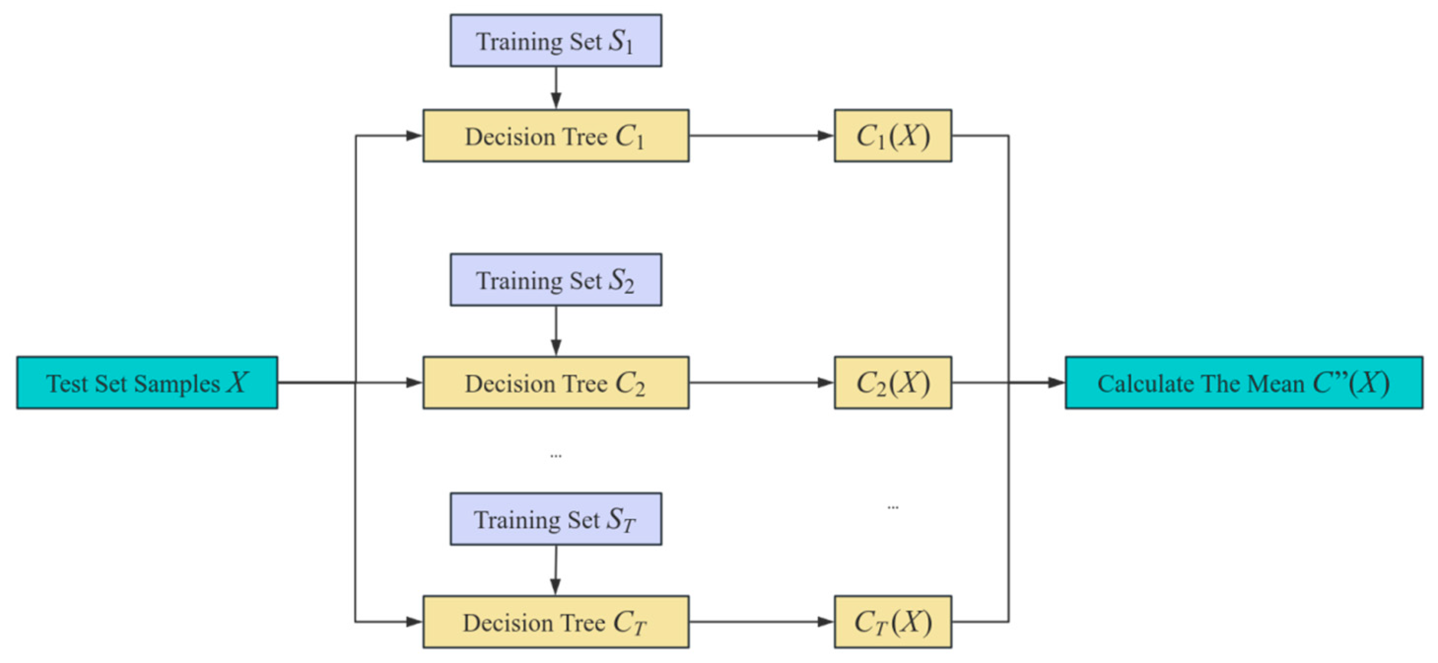
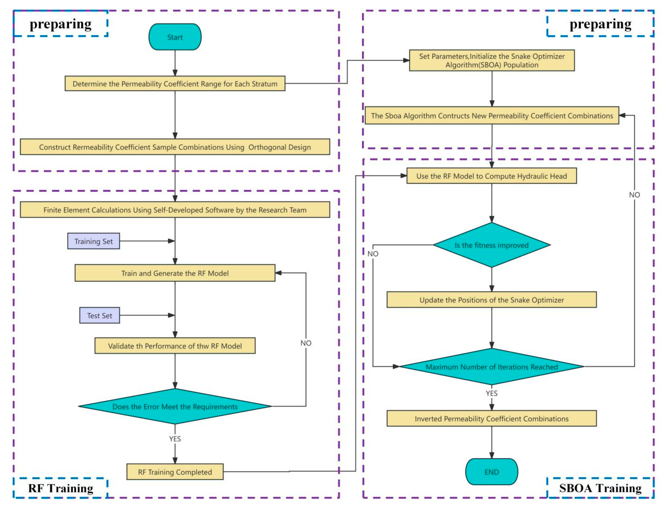
In response to these challenges, this study incorporates the Random Forest algorithm to develop a surrogate model for seepage analysis. The Random Forest algorithm offers high accuracy, strong noise resistance, and excellent capability in handling high-dimensional data. Also, it effectively prevents overfitting, demonstrates strong adaptability in regression tasks, and exhibits good robustness [35]. Compared to deep learning or other advanced machine learning models, Random Forest (RF) has lower computational complexity and better interpretability, making it particularly suitable for small sample data. Furthermore, to improve optimization efficiency, this paper introduces a swarm intelligence optimization algorithm—the Secretary Bird Optimization Algorithm—in the optimization process to establish an RF–SBOA intelligent inversion model for permeability coefficients. The feasibility and effectiveness of the proposed model are validated through a case study of the C-pumped storage power station.

2. Principles

2.1. Basic Principles of the Random Forest Algorithm

Random Forest is composed of numerous independent decision trees, and it forms the final prediction by aggregating the predictions of all the decision trees. It is an ensemble learning model based on the bagging strategy, which can effectively the handle nonlinear regression problem. The basic concept is illustrated in Figure 1, and it is executed according to the following four steps:

(1)

Let the training sample set be denoted as $S=\left\{x_1,x_1,\dots ,x_n\right\}$. Utilizing the bootstrap method, $n$ samples are drawn with replacement from $S$, resulting in the generation of $T$ new training datasets $S_i\left(i=1,2,\dots ,T\right)$. The total number of samples in each new dataset is the same as in $S$, but each dataset contains only about two-thirds of the samples from $S$.

(2)

Based on each training dataset $S_i(i=1, 2, \dots , T)$, generate the corresponding decision tree models $C_1$, $C_2$, …, $C_T$.

(3)

Each of the $T$ decision tree models is used to test the samples in the test set $X$, yielding corresponding results denoted as $C_1\left(X\right)$, $C_2\left(X\right)$, …, $C_T\left(X\right)$;

(4)

Compute the mean of the outputs from the decision tree models to obtain the final prediction result for $X$.

The Random Forest (RF) model has three key parameters: the number of decision trees $N_{tree}$, the number of random features considered for node splitting $M_{try}$, and the minimum number of samples required at the leaf nodes $Nod{e}_{size}$. Among these, $Nod{e}_{size}$ has a relatively minor impact on the performance, and the efficiency of the RF model is typically set to its default value. The underlying concept is illustrated in Figure 1 below.

2.2. Basic Principles of the Vulture Algorithm

The Secretary Bird Optimization Algorithm (SBOA) is an advanced metaheuristic algorithm, rooted in the survival strategies of the secretary bird and engineered to address complex real-world optimization problems [36]. This algorithm was proposed by Youfa Fu and others in April of this year.

Based on the biological statistics of the secretary bird’s predation stages and the duration of each stage, the entire predation process is divided into three equal time intervals: $t\le {\displaystyle \frac{1}{3}}T$, ${\displaystyle \frac{1}{3}}T\le t\le {\displaystyle \frac{2}{3}}T$, and ${\displaystyle \frac{2}{3}}T\le t\le T$. These intervals correspond to the three key phases of the secretary bird’s predatory behavior: searching for prey, consuming prey, and attacking prey.

2.2.1. Initialization Phase

In the SBOA method, the position of the secretary bird represents the candidate solution to the current problem. During the SBOA process, Equation (1) is employed to randomly initialize the position of the secretary bird within the search space.

$$X_{i,j}=l{b}_j+r\times (u{b}_j-l{b}_j),i=1,2,\dots ,N,j=1,2,\dots ,Dim$$

(1)

Let $X_i$ indicate the position of the $i$th secretary bird, $l{b}_j$ and $u{b}_j$ denote the lower and upper bounds, respectively, and $r$ indicate a random number within the range of 0 to 1.

2.2.2. Hunting Strategy of Secretary Bird

The hunting behavior of the secretary bird when preying on snakes is typically divided into three sub-actions: locating, consuming, and attracting.

(a)

Locating.

During the locating phase, the update of the secretary bird’s position can be modeled using Equations (2) and (3).

$$\mathit{While}t\le {\displaystyle \frac{1}{3}}T,x_{i,j}^{newP1}=x_{i,j}+(x_{random\_1}-x_{random\_2})\times R_1$$

(2)

$$X_i=\left\{\begin{array}{l}{X}_i^{new,P1},if F_i^{new,P1}\le F_i\\ X_i,else\end{array}\right.$$

(3)

Let $t$ denote the current iteration. $T$ represents the maximum number of iterations, $X_i^{new,P1}$ indicates the new state of the $i\mathrm{th}$ secretary bird in the first stage, and $x_{random\_1}$ and $x_{random\_2}$ are the random candidate solutions for the first-phase iteration. $R_1$ represents an array with dimensions $1\times Dim$ randomly generated with the interval [0, 1], where $Dim$ is the dimensionality of the solution space. $x_{i,j}^{newP1}$ denotes the value of the $j$th dimension, and $F_i^{new,P1}$ represents the fitness value of its objective function.

(b)

Consuming.

In this stage, the concept of ‘$x_{best}$’ (the historical best position) and Brownian motion (RB) are utilized. By employing ‘$x_{best}$’, individuals can conduct local searches around previously identified optimal positions, thereby facilitating a more thorough exploration of the surrounding solution space. The introduction of Brownian motion randomness enables individuals to explore the solution space more effectively and provides opportunities to avoid local optima, thus yielding better results when solving complex problems. Brownian motion can be modeled using Equation (4). The position updates during the predation phase can be modeled using Equations (5) and (6).

$$RB=randn(1,Dim)$$

(4)

$$\mathit{While}{\displaystyle \frac{1}{3}}T\le t\le {\displaystyle \frac{2}{3}}T,x_{i,j}^{newP1}=x_{best}+\exp ((t/T)\wedge 4)\times (RB-0.5)\times (x_{best}-x_{i,j})$$

(5)

$$X_i=\left\{\begin{array}{l}{X}_i^{new,P1},if F_i^{new,P1}\le F_i\\ X_i,else\end{array}\right.$$

(6)

Let $randn(1,Dim)$ denote a randomly generated array of dimension $1\times Dim$, randomly generated from a standard normal distribution (with a mean of 0 and a standard deviation of 1), and $x_{best}$ represents the current optimal value.

(c)

Attracting.

During the random search process, the integration of the Levy flight strategy enhances the optimizer’s global search capability, mitigates the risk of the SBOA converging to local solutions, and improves the algorithm’s convergence accuracy. The positions during the attack phase can be modeled using Equations (7) and (8).

$$\mathit{While}{\displaystyle \frac{2}{3}}T\le t\le T,x_{i,j}^{newP1}=x_{best}+((1-{\displaystyle \frac{t}{T}})\wedge (2\times {\displaystyle \frac{t}{T}}))\times x_{i,j}\times RL$$

(7)

$$X_i=\left\{\begin{array}{l}{X}_i^{new,P1},if F_i^{new,P1}\le F_i\\ X_i,else\end{array}\right.$$

(8)

2.2.3. Escape Strategy of Secretary Bird

The escape strategies of the secretary bird’s prey can be categorized into two main types: rapid escape and camouflage. A dynamic perturbation factor, denoted as ${\left(1-{\displaystyle \frac{t}{T}}\right)}^2$, is introduced. This dynamic perturbation aids the algorithm in achieving a balance between exploration, which involves searching for new solutions, and exploitation, which focuses on refining known solutions. By adjusting these factors, the level of exploration or exploitation can be enhanced at different stages. The model can be performed using Equations (9) and (10).

$$x_{i,j}^{new,P2}=\left\{\begin{array}{l}{C}_1:x_{best}+(2\times RB-1)\times {(1-{\displaystyle \frac{t}{T}})}^2\times x_{i,j},if rand\le r\\ C_2:x_{i,j}+R_2\times (x_{random}-K\times x_{i,j}),else\end{array}\right.$$

(9)

$$X_i=\left\{\begin{array}{l}{X}_i^{new,P2},if F_i^{new,P2}\le F_i\\ X_i,else\end{array}\right.$$

(10)

Here, r = 0.5. $R_2$ denotes an array with dimensions $1\times Dim$ randomly generated from a normal distribution, $x_{random}$ represents the random candidate solution in the current iteration, and $K$ indicates a randomly selected integer, either 1 or 2, which can be computed using Equation (11).

$$K=round(1+rand(1,1))$$

(11)

Here, $rand(1,1)$ means randomly generating a random number between 0 and 1.

A simplified SBOA flowchart is shown in Figure 2 below.

3. Permeability-Coefficient Inversion Model Based on RF–SBOA

3.1. The Fitness Function of the SBOA (Self-Balancing Optimization Algorithm)

The primary objective of seepage parameter inversion is to find the optimal values within their range, which is essentially an optimization problem. Therefore, optimization algorithms can be employed to solve this problem. This study employs the SBOA to search for the optimal permeability coefficients in the geological engineering area and establishes an inversion model based on RF–SBOA. During the inversion process, the fitness function for the SBOA is defined as the minimum mean-squared error (MSE) between the observed and calculated water levels at boreholes. The mathematical expression for this fitness function is provided in Equation (12).

$$f=\min MSE=\min \left[{\displaystyle \frac{1}{q}}{\displaystyle \sum _{k=1}^q{(H_k-H_k^{\prime })}^2}\right]$$

(12)

where $H_k$ represents the actual water-level measurement of the $k$th borehole, in meters (m); $H_k^{\prime }$ represents the finite element-calculated water level of the $k$th borehole, in meters (m); and $q$ denotes the total number of boreholes.

The constraint conditions of the objective function are given in Equation (13).

$$\mathrm{s}.\mathrm{t}. x_m^d\le x_m\le x_m^u (\mathrm{m}=1,2,\dots ,\mathrm{M})$$

(13)

where $x_m$ represents the permeability coefficient to be inverted, (m/s); $x_m^u$ and $x_m^d$ are the lower and upper bounds of the permeability coefficient, respectively, (m/s); and $M$ denotes the total number of permeability coefficients to be inverted.

3.2. Establishment of the RF–SBOA Inversion Model

This study establishes an inversion model for geological permeability coefficients in the engineering area based on the RF model and the SBOA. The model intelligently searches for the optimal values to accurately reflect the natural seepage characteristics of the area. The execution process of the inversion model is illustrated in the figure and is primarily completed in seven steps.

(1)

Generate permeability-coefficient combination samples using the orthogonal experimental method. Calculate the borehole water levels for each combination using the finite-element forward model. Establish an inversion sample set for the permeability coefficients.

(2)

Select 80% of the permeability-coefficient sample set as the training set, with the remaining 20% designed as the test set. In the RF model, define the input variables as permeability-coefficient combinations, while the output variable corresponds to the finite element-calculated borehole water levels. Simultaneously, the sample data are prepossessed using a normalization formula to constrain the variable data within the range [0, 1], thereby eliminating the influence of variable dimensions on the RF model. $x_m^{\prime }$ represents the normalized permeability-coefficient value.

$$x_m^{\prime }=(x_m-x_m^d)/(x_m^n-x_m^d)$$

(14)

(3)

Determine the optimal parameters $M_{try}$ and $N_{tree}$ of the RF model using ten cross-validations, and subsequently train the RF surrogate model.

(4)

Validate whether the training accuracy of the surrogate model established in step (3) meets the specified error threshold. If the accuracy satisfies the requirement, proceed to step (5); otherwise, repeat steps (3) and (4) until the threshold is met.

(5)

The output results are denormalized, and the performance of the surrogate model is evaluated using statistical metrics: mean absolute error (MAE), mean absolute percentage error (MAPE), root-mean-square error (RMSE), and the coefficient of determination ($R^2$).

(6)

During the SBOA search, the surrogate model iteratively calculates borehole water levels for newly generated permeability-coefficient combinations. If the fitness value for a given combination surpasses the current best fitness, the model updates the permeability-coefficient combination and fitness value to this new optimal state; otherwise, the process advances to step (7).

(7)

If the number of SBOA iterations has not yet reached the predefined maximum, repeat step (6). Otherwise, consider the current permeability-coefficient combination as the final inversion result and output it.

A simplified flow chart of the geological permeability coefficient inversion model is shown in Figure 3.

4. Engineering Case Study

4.1. Project Overview

A pumped storage power station is situated in Chongqing, China. It plays a critical role in the Chongqing power grid by performing tasks such as peak shaving, valley filling, energy storage, frequency regulation, voltage support, and providing emergency backup. The lower reservoir dam is a roller-compacted concrete gravity dam with a straight alignment of the dam axis, which is approximately orthogonal to the river flow. The elevation of the dam crest is 982 m, with the foundation elevation at the riverbed being 890 m, resulting in a maximum dam height of 92 m. The total length of the dam crest is 148 m, with a crest width of 8 m and a maximum base width of 68.10 m. The normal water level is 977 m, corresponding to a reservoir capacity of 10.77 m³.

The geological conditions in the lower reservoir’s catchment area are complex, featuring soluble rock layers that have undergone prolonged dissolution and erosional processes. This has led to the formation of a diverse array of subterranean karst landforms. The rock mass at the dam site of the lower reservoir is categorized into different layers based on rock type and permeability coefficients, including a weakly weathered layer, a strongly weathered layer, and a slightly altered rock mass. The geological cross-section of the riverbed is illustrated in Figure 4. The karst development in the reservoir area is notably intense, with numerous exposed caves and widespread surface dissolution phenomena. Vertical karst conduits are well-developed and align with the direction of structural lines, providing pathways for groundwater flow. This condition poses a risk of seepage around the dam, necessitating the implementation of effective seepage-control measures. The primary karst conduits in the reservoir area are illustrated in Figure 5. A schematic diagram of a typical borehole arrangement is shown in Figure 6.

4.2. Establishment of the Finite-Element Model

We define the coordinate system for the finite-element model as follows: the x-direction is aligned with the river flow direction, with positive values oriented downstream; the y-direction corresponds to the dam axis direction, with positive values directed towards the left bank; and the z-direction is the vertical axis, with positive values oriented upward. The computational model encompasses the entire lower reservoir structure and its impact area. The upstream and downstream boundaries are defined as follows: the upstream boundary extends approximately 200 m, equivalent to about 2.2 times the dam height, from the upstream toe of the lower reservoir’s concrete gravity dam. The downstream boundary extends approximately 155 m, equivalent to about 1.8 times the dam height, beyond the downstream apron. The left and right boundaries are defined as follows: the left boundary extends 265 m beyond the left abutment grout gallery. The right boundary extends 410 m beyond the right abutment grout gallery, encompassing the mountain masses on both sides. The top elevation is modeled according to the actual terrain, while the bottom elevation extends approximately 200 m, or about twice the dam height, below the foundation surface, reaching the slightly altered and fresh rock strata.

This study focuses on the detailed simulation of the strongly weathered layer, weakly weathered layer, slightly altered rock strata, and karst conduits within the lower reservoir site. The model was discretized using a mesh, resulting in the generation of 70,528 nodes and 70,632 elements. The prescribed hydraulic head boundaries are defined by the normal reservoir level of 977 m on the upstream side and a head boundary below 893 m on the downstream side. The seepage boundaries are represented by the water-level boundary of the Yangquan River channel. Impermeable boundaries are designated along the ground surface of the model and the lateral boundaries of the domain. The three-dimensional finite-element mesh division and boundary conditions are illustrated in Figure 7.

4.3. Rock Layer Permeability-Coefficient Inversion

4.3.1. Sample Construction Based on Orthogonal Design

In the inversion analysis, the permeability coefficients of each layer are considered isotropic, as detailed in

Table 1. Permeability-coefficient Ranges for Different Geological Layers.

Range of Rock Layers	Measure Range	Permeability Classification
Strongly Weathered Layer	1.00 × 10−8~1.00 × 10−7	Low Permeability
Weakly Weathered Layer	1.00 × 10−7~1.00 × 10−6	Weak Permeability
Slightly Altered Rock Mass	1.00 × 10−6~1.00 × 10−5	Very Low to Weak Permeability
Karst Caves	1.00 × 10−3~1.00 × 10−2	Extremely High Permeability

.

To ensure the accuracy of the RF model while not significantly increasing the computational workload of the finite-element forward analysis, this study employs a multi-factor, multi-level orthogonal design method to construct a representative sample set of permeability coefficients. The orthogonal table is a crucial component of orthogonal experimental design, typically denoted as $L_n\left(t^c\right)$. Here, $L$ represents the orthogonal table, $n$ indicates the total number of experimental runs, $t$ denotes the number of levels for each factor, and $c$ signifies the maximum number of factors that can be accommodated. For the micro-orthogonal experiment involving the permeability coefficients of the strongly weathered layer, weakly weathered layer, slightly altered rock mass, and karst conduits, each factor is assigned nine levels, as detailed in

Table 2. Permeability-coefficient Levels of Rock Layers Based on Orthogonal Design.

Level	Strongly Weathered Layer	Weakly Weathered Layer	Slightly Altered Rock Mass	Karst Conduits
1	1.00 × 10−8	1.00 × 10−7	1.00 × 10−6	1.00 × 10−3
2	2.13 × 10−8	2.13 × 10−7	2.13 × 10−6	2.13 × 10−3
3	3.25 × 10−8	3.25 × 10−7	3.25 × 10−6	3.25 × 10−3
4	4.38 × 10−8	4.38 × 10−7	4.38 × 10−6	4.38 × 10−3
5	5.50 × 10−8	5.50 × 10−7	5.50 × 10−6	5.50 × 10−3
6	6.63 × 10−8	6.63 × 10−7	6.63 × 10−6	6.63 × 10−3
7	7.75 × 10−8	7.75 × 10−7	7.75 × 10−6	7.75 × 10−3
8	8.88 × 10−8	8.88 × 10−7	8.88 × 10−6	8.88 × 10−3
9	1.00 × 10−7	1.00 × 10−6	1.00 × 10−5	1.00 × 10−2

. Therefore, the experimental samples are designed according to the orthogonal table $L_{81}\left(9^5\right)$, resulting in 81 combinations of permeability-coefficient schemes. On this basis, the finite-element forward model is used to calculate the water-level values for each permeability-coefficient combination, thereby constructing 81 sets of permeability-coefficient inversion samples. Among these sample, the first 80% of the dataset is selected as the training set to train the RF model, while the remaining 20% is used as the test set to validate the performance of the trained RF model.

4.3.2. Karst Region Seepage-Field Calculation Theory

The diversity of karst aquifer media determines the computational complexity of karst water-flow dynamics. This paper employs a self-developed finite-element forward calculation program based on the improved equivalent permeability method [37], which mathematically describes the non-Darcian flow behavior in karst media. This method can simultaneously reflect both laminar and turbulent flow types within the karst seepage field.

The fundamental differential equation for non-steady-state karst seepage incorporating the equivalent permeability coefficient is as follows:

$${\displaystyle \frac{\partial }{\partial x_i}}\left(k_{ij}{\displaystyle \frac{\partial h}{\partial x_j}}\right)=S_s{\displaystyle \frac{\partial h}{\partial t}}$$

(15)

where $k_{ij}$ represents the equivalent permeability tensor in the global coordinate system.

Combining the Galerkin finite-element method, the finite-element equation for seepage-field calculation in karst areas is as follows:

$$KP+(S+G)\left\{{\displaystyle \frac{\partial P}{\partial t}}\right\}=F$$

(16)

where $K$ represents the total permeability matrix; $P$ denotes the node pressure head array; $S$ is the storage matrix; $G$ refers to the water supply matrix; and $F$ signifies the imbalance flow array.

4.3.3. Validation of RF Model Performance

This study uses Borehole ZK118 as an example to evaluate the completeness, accuracy, and effectiveness of the RF model in the inversion of permeability coefficients. It also conducts a comparative analysis with classical models such as the classification and regression tree (CART), back propagation neural network (BP), and support vector regression (SVR). The prediction results of the RF, CART, BP and SVR models for the water level at Borehole ZK118 are shown in Figure 8 and Figure 9. Through ten-fold cross-validation, the optimal values for the RF parameters $N_{tree}$ and $M_{try}$ were determined to be 250 and 5, respectively. From Figure 8, it can be observed that the predicted curves of the four models are relatively close to the finite-element calculation curve, indicating a small prediction error. From Figure 9, it can be seen that the overall prediction residuals of the RF model are smaller than those of the CART, BP, and SVR models.

The prediction accuracy of the four models is quantitatively evaluated using the metrics MAE, MAPE, RMSE, and R². The detailed data are presented in

Table 3. Evaluation Metrics for the Prediction Results of Borehole ZK118 Water Levels by RF, CART, BP and SVR Models.

Model	Model Training				Model Validation
	MAE/m	MAPE/%	RMSE/m	R2	MAE/m	MAPE/%	RMSE/m	R2
RF	0.404	0.051	0.602	0.932	0.422	0.057	0.623	0.911
CART	0.666	0.063	0.778	0.921	0.678	0.068	0.795	0.897
BP	0.775	0.081	0.813	0.914	0.782	0.094	0.834	0.886
SVR	0.912	0.102	0.874	0.901	0.933	0.114	0.901	0.881

. From Table 3, it can be observed that the evaluation metrics of the RF model outperform those of the CART, BP, and SVR models. Specifically, the R² values for the training and test sets reach 0.932 and 0.911, respectively, and the other metrics also remain at relatively low levels. This indicates that the RF model has a significantly better fit to the calculated water levels of Borehole ZK118 and demonstrates higher predictive accuracy compared to the CART, BP, and SVR models.

To evaluate the generalization ability of the RF model, the test-sample water levels from boreholes ZK117, ZK116, and ZK115 were used for validation. The water-level prediction curves of the RF, CART, and BP models for these three boreholes are shown in Figure 10, Figure 11 and Figure 12. Among them, the RF model exhibited the smallest prediction errors for the water levels at all three boreholes. The trends of the prediction curves were also more consistent with the calculated water-level curves, indicating that the RF model demonstrates better robustness against noise and superior generalization ability compared to the other two models.

Table 4. Evaluation Metrics for the Prediction Results of Various Borehole Water Levels by RF, CART, BP and SVR Models.

Model	Borehole	Model Training				Model Validation
		MAE/m	MAPE/%	RMSE/m	R2	MAE/m	MAPE/%	RMSE/m	R2
RF	ZK117	0.458	0.050	0.573	0.923	0.559	0.061	0.787	0.912
	ZK116	0.437	0.048	0.543	0.934	0.486	0.053	0.559	0.931
	ZK115	0.426	0.046	0.519	0.938	0.428	0.046	0.525	0.937
CART	ZK117	0.962	0.106	1.112	0.869	0.683	0.075	0.869	0.907
	ZK116	0.542	0.059	0.693	0.912	0.577	0.063	0.675	0.911
	ZK115	1.026	0.110	1.116	0.864	1.203	0.129	1.304	0.861
BP	ZK117	1.033	0.114	1.265	0.847	0.840	0.092	0.983	0.907
	ZK116	0.706	0.077	0.844	0.903	0.673	0.074	0.820	0.915
	ZK115	0.811	0.087	0.937	0.896	0.463	0.050	0.618	0.932
SVR	ZK117	0.874	0.096	1.095	0.889	1.065	0.117	1.161	0.856
	ZK116	0.883	0.097	1.014	0.894	0.537	0.059	0.610	0.922
	ZK115	0.472	0.051	0.568	0.927	0.471	0.051	0.569	0.927

presents the evaluation metrics for the RF, CART, BP, and SVR models in predicting water levels at boreholes ZK117, ZK116, and ZK115. As shown in Table 4, the R² values of the RF model for the three boreholes are 0.912, 0.931, and 0.937, respectively. This indicates that the RF model exhibits superior generalization performance compared to the other models, demonstrating a markedly stronger ability to predict water levels accurately across the test sets.

In summary, the RF model developed in this study demonstrates superior performance at all six borehole locations, accurately predicting the borehole water levels. Thus, the RF model exhibits better predictive accuracy, generalization capability, and robustness, making it a suitable surrogate model for the inversion of seepage parameters.

4.3.4. Permeability-Coefficient Inversion Based on the SBOA

Based on the validation of the RF surrogate model’s accuracy, this study employs the SBOA for the global optimization of permeability coefficients. The optimal permeability coefficients for each geological layer and karst conduit obtained through inversion are presented in

Table 5. The inversion results of permeability coefficients.

Strata Range	Inversion Value (cm/s)	Permeability Classification
Highly Weathered Layer	1.26 × 10−4	Weakly Permeable
Weakly Weathered Layer	1.17 × 10−5	Weakly Permeable
Slightly New Rock Mass	1.30 × 10−6	Extremely Low to Weakly Permeable
Karst Conduit	1.10 × 10−1	Extremely Highly Permeable

.

To validate the reasonableness of the inverted permeability coefficients, these coefficients are substituted into the finite-element forward model to complete the water level at each borehole. The computed water levels are them compared with the measured water levels. The comparison results are presented in the

Table 6. Comparison between Measured and Inverted Water Levels of Boreholes.

Borehole	Calculated Water Level	Measured Water Level	Absolute Error/m	Relative Error/%
ZK118	914.11	913.04	1.07	0.117
ZK117	911.89	911.66	0.23	0.025
ZK116	912.42	911.50	0.92	0.101
ZK115	929.77	928.58	1.19	0.128

.

To further demonstrate the competitiveness of the inversion model, RF–PSO, RF–GWO, and RF–SSA were also employed to perform inversion analysis on the material with undetermined permeability coefficients. The relative errors between the predicted and actual borehole water levels, calculated using a finite-element model, are shown in

Table 7. Relative errors of the models.

Model	Borehole with the Largest Error	Absolute Error/m	Relative Error/%	Training Time/s
RF–SBOA	ZK115	1.19	0.117	0.74
RF–PSO	ZK118	4.78	0.47	1.25
RF–GWO	ZK115	3.88	0.38	1.68
RE-SSA	ZK115	2.74	0.26	2.27

. The relative error based on the RF–SBOA model in Table 7 is the smallest, indicating that this model has a clear advantage over other traditional intelligent algorithm models in seepage parameter-inversion analysis. Meanwhile, the built-in MATLAB timing function was used to compare the training times of the four models mentioned above. The RF–SBOA model had the shortest training time for sample data at 0.74 s. This clearly demonstrates that RF–SBOA also has a faster convergence speed during sample data training compared to the other models.

4.4. Analysis of Groundwater Flow Field

4.4.1. Natural Period

Figure 13 illustrates the distribution of groundwater-head contour lines within the model calculation area. It is evident from Figure 13 that the groundwater level is relatively lower near the river channel and dam site area, while it is higher in the mountainous areas towards the riverbed. Within the dam site area, the groundwater level decreases progressively from the mountainous areas towards the riverbed. The contour lines of groundwater levels on the left bank are denser, indicating a steeper hydraulic gradient, whereas those on the right bank are sparser, reflecting a gentler gradient. The groundwater level in the dam-site area is lower and more gradual near the river channel, with higher and more rapidly changing levels on the left bank. The presence of karst channels causes rapid changes in the groundwater-level contour lines within the distribution area, leading to a steeper hydraulic gradient and faster decline in groundwater levels. The simulation results show that the groundwater gradient in the right bank’s mountainous area is relatively uniform, with a smaller gradient near the river channel, resulting in a more gradual change in groundwater levels. The groundwater flow and level distribution within the calculation domain align with engineering principles and are consistent with the topographical and geological conditions. The finite-element model effectively simulates the engineering geological conditions of the hub area and the permeability zoning of the rock mass. The distribution of the natural groundwater seepage field in the simulation is generally consistent with the actual conditions observed during investigations.

4.4.2. Normal Storage-Level Operational Period

Under the normal reservoir water level, the contour map of groundwater levels is shown in Figure 14, and the maximum cross-sectional groundwater-level contours are shown in Figure 15. The potential distribution pattern of the seepage field after reservoir filling is clear: on the right bank, the groundwater level outside the seepage cutoff curtain is 10 m higher than the normal reservoir water level, at 985 m; on the left bank, the groundwater level outside the seepage cutoff curtain is 10 m lower than the normal reservoir water level, at 965 m. The presence of underground caverns on the right bank, which are intercepted by the seepage cutoff curtain, results in an uneven distribution of groundwater-level contours between the left and right banks, with minor seepage occurring at the dam foundation.

The permeation flow and permeation gradient at various locations in the reservoir area are presented in

Table 8. Results of Calculations During Normal Reservoir Water-level Period (Where Average permeation gradient is only considered for impermeation curtains).

Rock Layer	Permeation Flow (m3/d)	Average Permeation Gradient	Location
Left Bank Curtain	234.56	10.22	Downstream groundwater surface beneath the left dam segment curtain
Left Bank Bedrock	896.73	——	——
Riverbed Curtain	352.37	19.64	Top of the highest dam slope curtain in the riverbed
Riverbed Bedrock	675.24	——	——
Right Bank Curtain	289.93	11.09	Near the downstream groundwater surface beneath the right dam end curtain
Right Bank Bedrock	984.52	——	——
Total Permeation Flow	3433.35	——	——

. During the normal water-level period, the total permeation flow of the reservoir is 3433.35 m³/d, with the riverbed permeation flow accounting for 34% of the total. Given that the hydraulic conditions reflect stable seepage, the preliminary seepage-control plan shows that the permeation flow through the dam body and dam foundation drainage holes are 110.5 m³/d and 112.7 m³/d, respectively. The maximum average permeation gradients are within the regulatory range of 10–30, indicating that the results derived from the inversion parameter calculations align with engineering experience and meet the standard requirements.

5. Conclusions

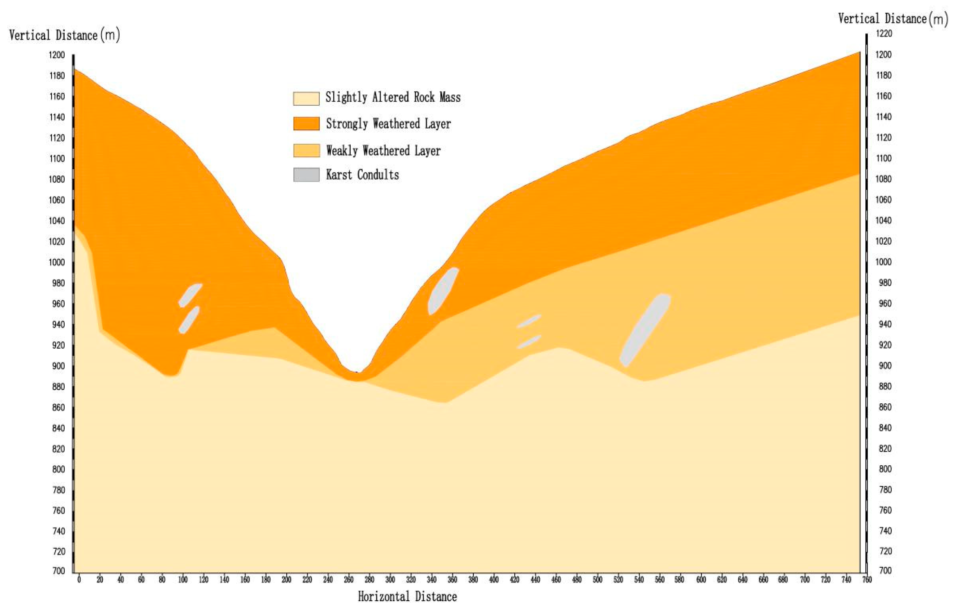
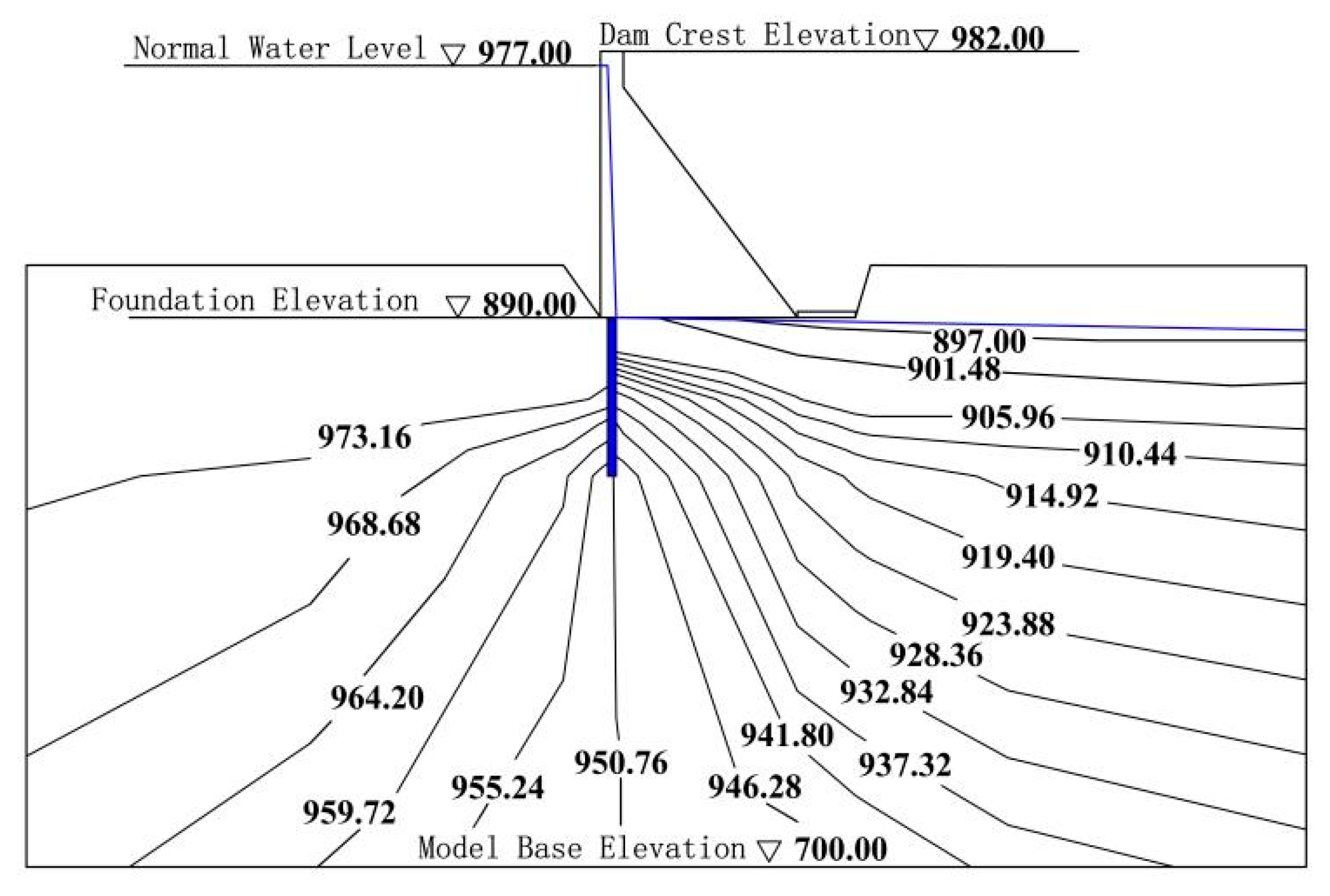
This paper establishes an intelligent inversion model for geological permeability coefficients based on the RF–SBOA. The model successfully addresses the inversion problem of geological permeability coefficients for the C-pumped storage power station, revealing the overall distribution characteristics of its natural seepage field and validating the reasonableness of seepage flow and permeability gradient under normal water-storage conditions.

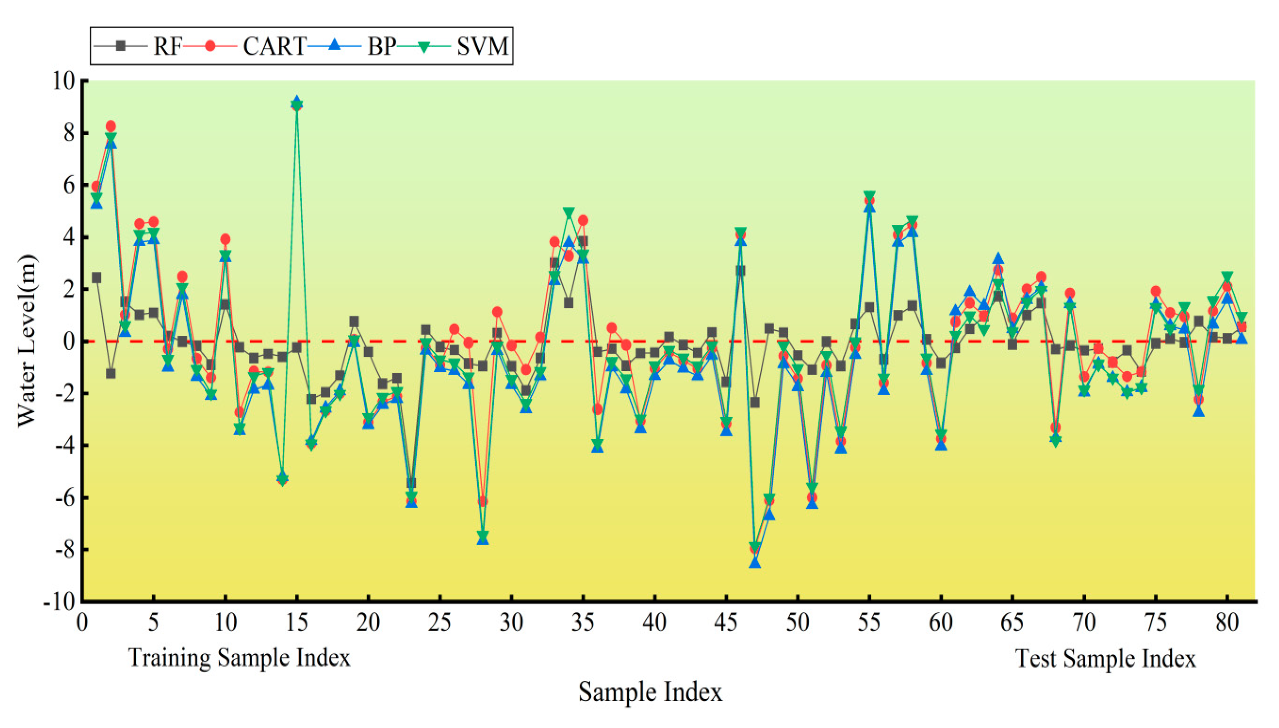
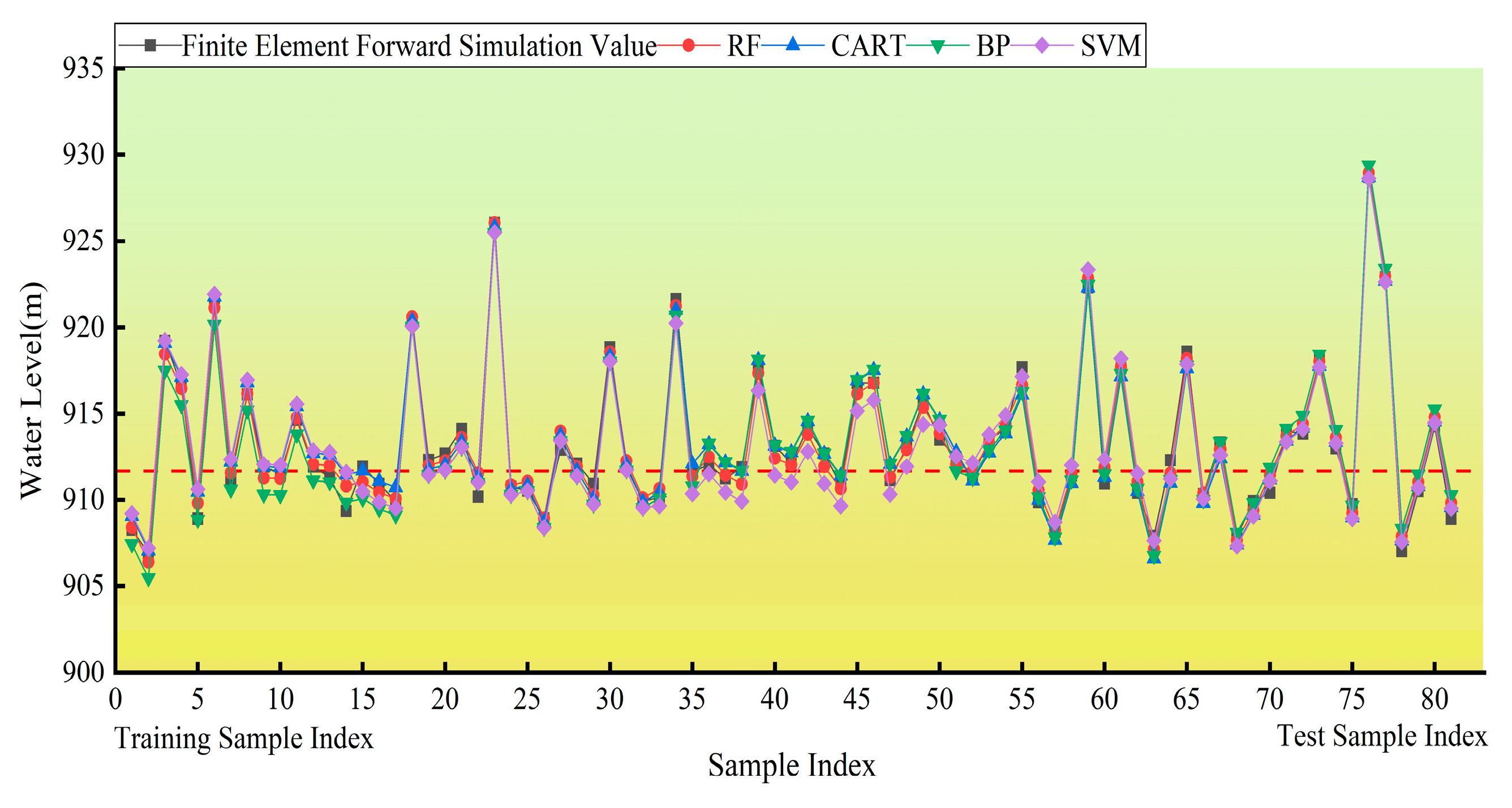
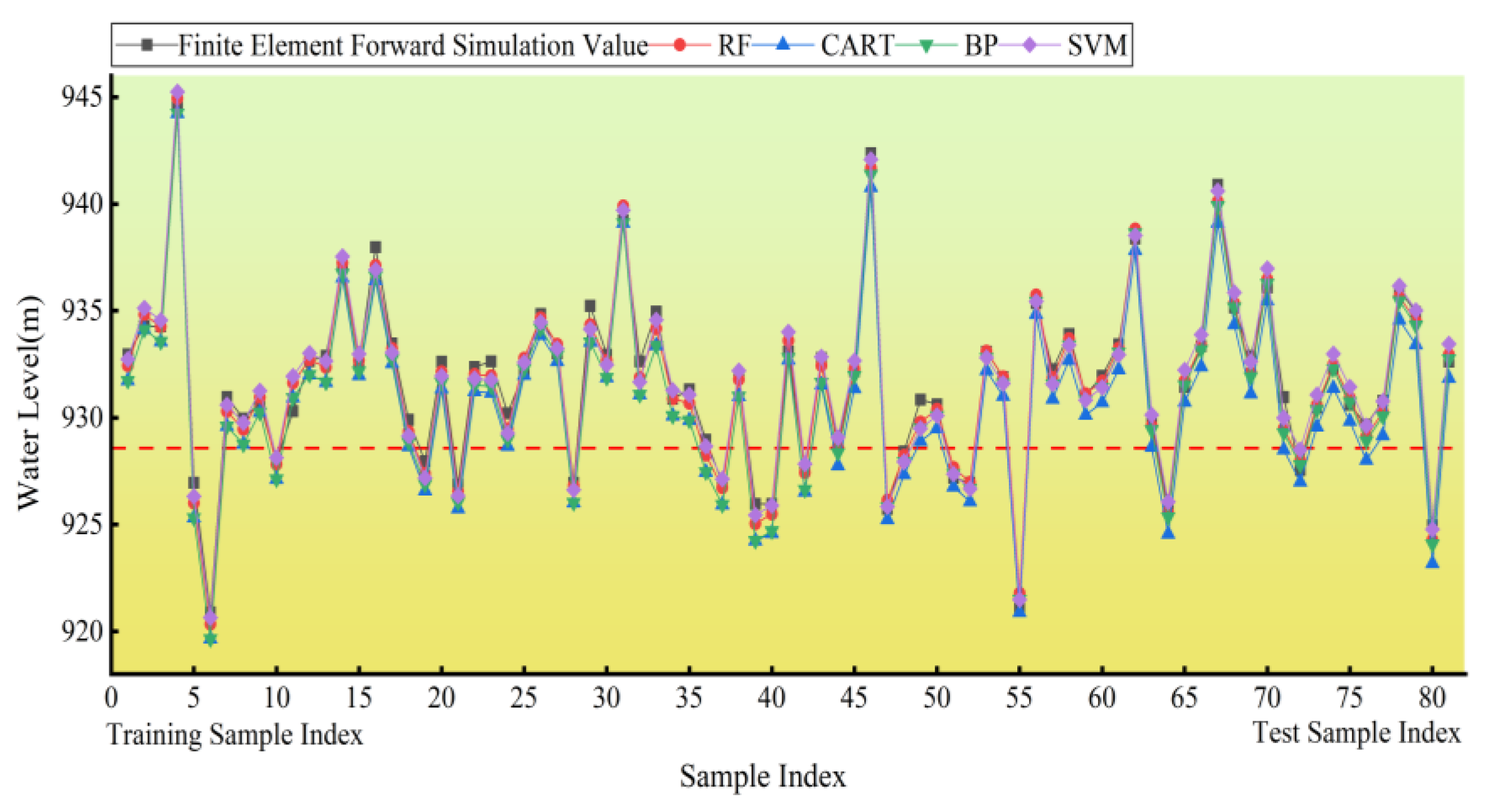
By comparing with the CART, BP, and SVR models, the RF model provides borehole water-level predictions that are closer to the finite-element computation values and demonstrates the lowest performance evaluation metrics. This indicates that the RF model has superior predictive accuracy and generalization capability. Therefore, it can serve as an alternative to the finite-element forward model for seepage calculations, significantly reducing the need for extensive finite-element forward computations.

The introduction of the SBOA enhances the RF model’s global search capability and optimization efficiency, improving the ability to identify the optimal geological permeability coefficients. The inversion results for borehole water levels are reasonable, with the maximum absolute and relative errors aligning with engineering experience. In comparison with RF–PSO, RF–GWO, and RF–SSA surrogate models, the RF–SBOA demonstrates faster optimization efficiency, stronger global search capabilities, and lower errors. The calculated distribution of the natural seepage field is consistent with the general patterns observed in mountainous seepage fields. Considering the dam body and curtain grouting, during the operational period under normal water-storage conditions, the seepage flow and seepage gradient meet regulatory standards.

The introduction of the RF–SBOA improves the efficiency of the inversion process and offers strong potential for future applications in engineering geological inversion. However, there is still room for improvement. Firstly, this study only employs data from a single borehole in the project area to model and invert the optimal geological permeability coefficient. Determining how to utilize the relationships between different boreholes in modeling requires further research. Secondly, while the accuracy of the RF–SBOA is sufficient for permeability-coefficient inversion in engineering areas, whether it has broader applicability in other fields, such as material parameter inversion in static and dynamic calculations, still needs further investigation and validation.

References

1. Guo, F.; Jiang, G.; Yuan, D.; Polk, J.S. Evolution of Major Environmental Geological Problems in Karst Areas of Southwestern China. Environ. Earth Sci. 2013, 69, 2427–2435. [Google Scholar] [CrossRef]
2. Yu, B.; Xu, G. Research on Rock Quality Detection of Dam Foundation in Guangzhao Hydropower Station. Chin. J. Rock Mech. Eng. 2008, 27 (Suppl. S1), 2883–2892. (In Chinese) [Google Scholar]
3. Dai, K.; Long, D.; Zhou, Z. Rapid Construction Techniques in Concrete Arch Dam Construction of Goupitan Hydropower Project. J. Hydraul. Eng. 2007, (Suppl. S1), 43–48. (In Chinese) [Google Scholar] [CrossRef]
4. Zhou, W.; Hua, J.; Chang, X.; Zhou, C. Settlement Analysis of the Shuibuya Concrete-face Rockfill Dam. Comput. Geotech. 2011, 38, 269–280. [Google Scholar] [CrossRef]
5. Ghobadi, M.H.; Khanlari, G.R.; Djalaly, H. Seepage Problems in the Right Abutment of the Shahid Abbaspour Dam, Southern Iran. Eng. Geol. 2005, 82, 119–126. [Google Scholar] [CrossRef]
6. Lin, C.; Li, L.; Han, X. Research on Forecast Method of Tunnel Water Inrush in Complex Karst Areas. Chin. J. Rock Mech. Eng. 2008, 27, 1469–1476. (In Chinese) [Google Scholar]
7. Galvao, P.; Halihan, T.; Hirata, R. The Karst Permeability Scale Effect of Sete Lagoas, MG, Brazil. J. Hydrol. 2016, 532, 149–162. [Google Scholar] [CrossRef]
8. Youssef, A.A.; Awotunde, A.A. Modelling Fluid Flow in Karst Reservoirs Using Darcy Model with Estimated Permeability Distribution. Comput. Geosci. 2019, 133, 104311. [Google Scholar] [CrossRef]
9. Malkawi, A.H.; Al-Sheriadeh, M. Evaluation and Rehabilitation of Dam Seepage Problems: A Case Study of Kafrein Dam. Eng. Geol. 2000, 56, 335–345. [Google Scholar] [CrossRef]
10. Mozafari, M.; Raeisi, E.; Zare, M. Water Leakage Paths in the Doosti Dam, Turkmenistan and Iran. Environ. Earth Sci. 2012, 65, 103–117. [Google Scholar] [CrossRef]
11. Gutiérrez, F.; Mozafari, M.; Carbonel, D.; Gómez, R.; Raeisi, E. Leakage Problems in Dams Built on Evaporites: The Case of La Loteta Dam (NE Spain), a Reservoir in a Large Karstic Depression Generated by Interstratal Salt Dissolution. Eng. Geol. 2015, 185, 139–154. [Google Scholar] [CrossRef]
12. Wang, H.; Xu, W.; Yu, H. Seepage Analysis of Fracture Network of Rock Mass in Karst Area. Rock Soil Mech. 2005, 26, 1080–1084. (In Chinese) [Google Scholar]
13. Li, S.; Shi, S.; Li, L.; Chen, J.; Xv, H.; Zhou, Z.; Yuan, Y. Control of Water Inrush in Typical Karst Tunnels in Three Gorges Reservoir Area and Its Application. Chin. J. Rock Mech. Eng. 2014, 33, 1887–1896. (In Chinese) [Google Scholar]
14. Huang, B.; Yin, Y.; Zhang, Z.; Wang, J.; Qin, Z.; Yan, G. Study on Deterioration Characteristics of Shallow Rock Mass in the Water Level Fluctuation Zone of Karst Bank Slopes in Three Gorges Reservoir Area. Chin. J. Rock Mech. Eng. 2019, 38, 1786–1796. (In Chinese) [Google Scholar]
15. Cao, W.; Ma, L.; Su, H. Inversion Method for Concrete Gravity Dam Parameters Based on MTSVR-ISAO [J/OL]. J. Hydroelectr. Eng. 2024. Available online: http://kns.cnki.net/kcms/detail/11.2241.TV.20240427.1704.004.html (accessed on 10 September 2024).
16. Xu, S.H.; Zhao, Y.C.; Wu, D.D.; Su, K. Research on the inversion method of mud permeability coefficient during the construction of earthwork cofferdam seepage control wall. China Rural. Water Hydropower 2024, 7, 177–182. [Google Scholar] [CrossRef]
17. Li, Y.; Shen, Z.; Xiong, H.; Li, H.; Zhang, H. Inversion Method and Application of Seepage Parameters for Core Rockfill Dams Based on LHS-ISSA-SVR. Water Power Energy Sci. 2024, 42, 109–113. [Google Scholar]
18. Moursi, W.M. The forward–backward algorithm and the normal problem. J. Optim. Theory Appl. 2018, 176, 605–624. [Google Scholar] [CrossRef]
19. Li, S.; Peissig, J. Measurement of head-related transfer functions: A review. Appl. Sci. 2020, 10, 5014. [Google Scholar] [CrossRef]
20. Sheng, J.C.; Su, B.Y.; Zhan, M.L. Inversion Analysis and Engineering Application of Three-Dimensional Natural Seepage Field. Chin. J. Rock Mech. Eng. 2003, 203–207. [Google Scholar]
21. Duan, B.; Zhang, L.; He, J.; Fu, W.; Chen, G. Inversion analysis of natural seepage field in complex fractured rock masses. J. Hydroelectr. Eng. 2012, 31, 188–193+198. [Google Scholar]
22. Hu, P.; Wen, Z.; Hu, X.; Zhang, Y. Inversion of Landslide Permeability Coefficient Based on Genetic Algorithm-Support Vector Machine. Hydrogeol. Eng. Geol. 2021, 48, 160–168. [Google Scholar] [CrossRef]
23. Liu, H.; Liu, H.; Li, L.; Chen, X.; Che, J.; Yang, W. Prediction of Compressive Strength of Desert Sand Concrete After High Temperature Based on Improved BP Model [J/OL]. J. Henan Polytech. Univ. (Nat. Sci. Ed.) 2024. Available online: http://kns.cnki.net/kcms/detail/41.1384.N.20240909.1332.004.html (accessed on 10 September 2024).
24. Hu, Y.; Li, S. Research on Optimized Extreme Learning Machine Model for Classification of Steel Plate Surface Defects [J/OL]. Comput. Appl. Softw. 2024. Available online: http://kns.cnki.net/kcms/detail/31.1260.tp.20240829.1800.005.html (accessed on 10 September 2024).
25. Yang, Q.; Zhong, W.; Xie, S.; Zhou, G. Frequency Control of Offshore Wind Power VSC-HVDC Grid Connection System Based on Particle Swarm Optimization of PID [J/OL]. Autom. Technol. Appl. 2024, 2–6. Available online: http://kns.cnki.net/kcms/detail/23.1474.tp.20240816.1902.001.html (accessed on 10 September 2024).
26. Pan, W.; Zhao, T.; Li, X.; Lu, Y. Landslide Susceptibility Assessment in Loess Areas Based on Multivariate Adaptive Regression Splines. Res. Soil Water Conserv. 2024, 31, 271–280. [Google Scholar] [CrossRef]
27. Xu, L.; Shen, Z. An ELM-GA-Based Inversion Model for the Permeability Coefficient of Complex Rockfill Dams and Its Application. Hydropower Energy Sci. 2021, 39, 86–90. [Google Scholar]
28. Qian, W. Research on the Inverse Problem of Seepage Field Based on Differential Evolution Algorithm and Reduced-Order Model. Ph.D. Thesis, Xi’an University of Technology, Xi’an, China, 2020. [Google Scholar] [CrossRef]
29. He, Y.; Huang, Y.; Fei, D.; Gao, D.; Yang, M. Inverse Analysis of Time-Dependent Permeability Coefficient of Composite Geomembranes in Wang Fuzhou Water Conservancy Project. Water Resour. Hydropower Eng. 2022, 53, 112–120, (In Chinese and English). [Google Scholar] [CrossRef]
30. Lei, Y.; Wen, L.F.; Zhao, M.C.; Yin, Q. Intelligent Inversion Analysis of Geological Permeability Coefficients in Hydraulic Engineering Based on RF-GWO. J. Water Resour. Water Eng. 2024, 35, 139–148. [Google Scholar]
31. Gaur, H.; Khidhir, B.; Manchiryal, R.K. Solution of structural mechanic’s problems by machine learning. Int. J. Hydromechatronics 2022, 5, 22–43. [Google Scholar] [CrossRef]
32. Liu, B.K.; Lu, W.Z. Surrogate models in machine learning for computational stochastic multi-scale modelling in composite materials design. Int. J. Hydromechatronics 2022, 5, 336–365. [Google Scholar] [CrossRef]
33. Khalil, Z.H.; Khaleel, A.H. Design of a Multilayer Perceptron Network Based on the Normalized Histogram to Develop Yields Predictive Model. J. Data Sci. Intell. Syst. 2023. [Google Scholar] [CrossRef]
34. Chao, Q.; Xu, Z.; Shao, Y.; Tao, J.; Liu, C.; Ding, S. Hybrid model-driven and data-driven approach for the health assessment of axial piston pumps. Int. J. Hydromechatronics 2023, 6, 76–92. [Google Scholar] [CrossRef]
35. Ayua, S.I. Random Forest Ensemble Machine Learning Model for Early Detection and Prediction of Weight Category. J. Data Sci. Intell. Syst. 2023. [Google Scholar] [CrossRef]
36. Fu, Y.; Liu, D.; Chen, J.; He, L. Secretary bird optimization algorithm: A new metaheuristic for solving global optimization problems. Artif. Intell. Rev. 2024, 57, 123. [Google Scholar] [CrossRef]
37. Ji, W.; Zhao, J.; Shen, Z.Z.; Sun, Y. Study on the Optimization Layout of Anti-Seepage Curtain in Karst Body of Shuibuya Hydraulic Hub. Hydropower Energy Sci. 2005, 1, 36–39+91. [Google Scholar]
Figure 1. The Basic Principle of the Bagging Algorithm.
Water 16 03096 g001
Figure 2. Simplified flowchart for the SBOA.
Water 16 03096 g002
Figure 3. Simplified Flowchart for the Geological Permeability-coefficient Inversion Model.
Water 16 03096 g003
Figure 4. Cross-sectional geology of the riverbed.
Water 16 03096 g004
Figure 5. The main karst channel in the reservoir area.
Water 16 03096 g005
Figure 6. Schematic Diagram of Typical Borehole Arrangement.
Water 16 03096 g006
Figure 7. Mesh Generation and Boundary Conditions of the 3D Finite-element Model.
Water 16 03096 g007
Figure 8. Prediction Results of Borehole ZK118 Water Levels by RF, CART, BP, and SVR Models.
Water 16 03096 g008
Figure 9. Prediction Residual Results of Borehole ZK118 Water Levels by RF, CART, BP, and SVR Models.
Water 16 03096 g009
Figure 10. Prediction Results of Borehole ZK117 Water Levels by RF, CART, BP, and SVR Models.
Water 16 03096 g010
Figure 11. Prediction Results of Borehole ZK116 Water Levels by RF, CART, BP, and SVR Models.
Water 16 03096 g011
Figure 12. Prediction Results of Borehole ZK115 Water Levels by RF, CART, BP, and SVR Models.
Water 16 03096 g012
Figure 13. Contour Map of Natural Groundwater Levels.
Water 16 03096 g013
Figure 14. Contour Map of Groundwater Levels during Normal Reservoir Operation Period.
Water 16 03096 g014
Figure 15. Contour Map of Maximum Groundwater Levels during Normal Reservoir Operation Period.
Water 16 03096 g015