Real-Time Analysis and Digital Twin Modeling for CFD-Based Air Valve Control During Filling Procedures

Abstract

Air exchange in pressurized water pipelines is an essential but complex aspect of pipeline modeling and operation. Implementing effective air management strategies can yield numerous benefits, enhancing the system’s energy efficiency, reliability, and safety. This paper comprehensively evaluates an irregular profile pipeline filling procedure involving air-release through an air valve. The analysis includes real-time data tests and numerical simulations using Computational Fluid Dynamics (CFD). A Digital Twin model was proposed and applied to filling maneuvers in water installations. In particular, this research considers an often-overlooked aspect, such as filling a pipe with an irregular profile rather than a simple straight pipe. CFD simulations have proven to capture the main features of the transient event, which are suitable for tracking the air-water interface, the unsteady water flow, and the evolution of the trapped air pocket. Thus, they provide thorough and reliable information for real-time operational processes in the industry, focusing on the filling pressure and geometry of the air-valve hydraulic system. Additionally, this study provides details regarding the application of an efficient Digital Twin CFD approach, demonstrating its feasibility in optimizing the filling procedure in pipes with irregular profiles.

1. Introduction

Entrapped air in water pipelines encompasses a range of complex hydraulic and thermodynamic behaviors that must be studied. These interactions can affect the pipeline’s structural integrity and hydraulic devices [1]. Sub-atmospheric pressures pose risks for unburied large-diameter and thin-walled pipes [2]. Pressure surges can increase the probability of pipe ruptures [3,4], especially in old pipes [5]. Effects resulting from the interaction between water and air within a pipeline include the following: (i) a reduction in pipeline water conveyance capacity due to entrapped air, which restricts the cross-sectional area available for the water phase [6]; (ii) alterations in the physical and chemical properties of the conveyed water [7]; (iii) movement of air pockets along the pipeline from low to high points; (iv) fluctuations in air pocket volume and pressure; and (v) temperature during transient events [8].

During pipeline filling maneuvers, pressure surges can be attributed to two primary reasons. First, for having undersized or absence of air valves in hydraulic installations, where water columns rapidly compress entrapped air pockets. The second reason corresponds to when a water column closes the orifice of air valves by its high velocity, producing a second pressure surge that, in some cases, can deliver higher peaks of air pocket pressure compared to the first scenario. Consequently, filling procedures must be carefully performed with recommended water velocities and differential pressures [9]. In addition, these processes should be performed slowly and using well-sized air valves, which is crucial to mitigate dangerous transient oscillations [10].

Air/vacuum valves are used for filling and draining operations, while air-release valves are responsible for expelling small air bubbles during normal operation of water distribution systems [11]. For sizing purposes, it should be noted that air valve capacity depends on its orifice size and internal configuration. Air valve flow depends on the differential pressure, which can be modeled using the information provided by the manufacturer. It is also essential to select a reliable manufacturer with tested air valve capacity curves [12].

Different authors have developed mathematical models to understand the dynamic behavior of trapped air pockets in pipelines. Zhou et al. (2002) [13] studied air trapped in pipes with orifice sizes, identifying pressure oscillation patterns and the resulting pressure surges during rapid filling processes. De Martino et al. (2008) [14] developed a predictive equation derived from upstream conditions, orifice size, and pumping pressures of a water pipeline, establishing two phases of pressure oscillation: (i) an initial with low frequency during air-release and (ii) an overpressure caused by water hammer phenomena. Carlos et al. (2011) [15] studied the impact of trapped air on pipeline water transients using tests and a numerical model calibrated in experimental facilities, which can be used to predict the dynamic effects of air-release through different air valves and the overpressure that can cause damage in water distribution networks. Fuertes-Miquel et al. (2016) [16] analyzed the behavior of air when expelled through air valves through a mathematical model, focusing on the variation of isothermal and adiabatic conditions, impacting the effects of water hammers when water columns abruptly close air valves. Coronado-Hernández et al. (2019) [17] developed a rigid column mathematical model to simulate the filling of water pipelines with air valves, capturing hydraulic and thermodynamic variables and considering different physical equations such as the mass oscillation formula, air-water interface position, and the polytropic equation. Zhou et al. (2019) [18] investigated air expulsion in a vertical pipe through a mathematical model of elastic water columns, where they studied two stages of the filling processes: (i) pressurization of trapped air and (ii) water hammer impact. In addition, they explored different orifice sizes, observing air-damping effects in pipes with small orifices and dominant water hammer pressure in larger orifices. Romero et al. (2020) [19] presented a mathematical model to analyze pressure changes during the filling of hydraulic systems, focusing on large-scale pipelines. This mathematical model was initially validated by Coronado-Hernández et al. (2019) [17], and they were applied to pipelines with DN400 and DN600 [19]. The application to actual cases helped to understand transient events during filling processes. Zhou et al. (2019) [18] studied the expulsion of air through air valves in detail. In addition, they developed a mathematical model that considered the effects of trapped air and the water hammer phenomenon, which allowed a better understanding of the process and the factors that influence it.

A detailed understanding of the behavior of expelled air in pressurized pipelines.

Computational Fluid Dynamic (CFD) models have been complex, and information about this phenomenon is rarely available and focused on two essential aspects: expelled air in horizontal stormwater pipes with free surface flows and pressurized air using three-dimensional (3D) CFD models. For example, Li et al. (2018) [20] used a 3D CFD model to examine air-water interactions for expelled air in a horizontal pipe with trapped air during a rapid filling, revealing complex flow features and pressure patterns based on orifice position. Chan et al. (2018) [21] developed a 3D CFD model to study geysers in stormwater systems. They studied geyser formation through the dynamics of air pockets during the expulsion of air from horizontal hydraulic sections to vertical pipes. Wang and Vasconcelos (2018) [22] developed 3D CFD simulations of a stormwater pipeline with pressurized air in which it was shown that large air pocket leaks generated pressure spikes that exceeded roof displacement thresholds, offering ideas for managing air at stormwater crossings and avoiding operational problems. Fang et al. (2022) [23] developed a 3D CFD model applying the VOF method to simulate air-water interaction in T-junction stormwater pipes. They appropriately replicated experimental pressure oscillations, identifying air movement and expulsion in vertical pipes without geysers and air expulsion and critical geyser formation.

On the other hand, the movement and expelled air flow in pipelines of irregular profiles have been scarcely studied through 2D CFD models [24], where 2D CFD models have been developed to study rapid filling processes in pressurized pipes with single entrapped air pockets. These models helped us understand the influence of air valve sizing on controlling water hammer phenomena and the effects of different commercial air valves.

The advent of extensive data analysis and digitalization is transforming water infrastructure, necessitating standardization and systems that ensure the security of drinking water pipelines. In this context, Digital Twin technology is being deployed in water distribution systems to manage water leakages and assist with design purposes. However, the current literature needs more specific documentation for predicting filling operations. Since previous research has focused on traditional 2D CFD models that predict only physical patterns of hydraulic and thermodynamic parameters as well as contour analysis, this work contributes to the presentation of a 3D CFD model that combines real-time data integration from big data analysis techniques—leveraging sensor technology linked to safety devices like air valve operations during the start-up of water pipelines. The proposed model can be used to have additional analysis as follows: (i) a comprehensive study of the hydraulic and thermodynamic behaviors of air-water interaction during rapid filling and air expelling processes in irregular pipes with different branches and different air pocket sizes; and (ii) a three-dimensional analysis of the effects of expelled air on the proper management of trapped air during filling maneuvers. Real-time data and numerical analysis are performed in this research through an experimental setup, which is carried out to represent different filling processes through a pipeline with horizontal and diagonal branches where different tests are performed with an air valve and different initial hydraulic conditions. A three-dimensional CFD model of the experimental setup is developed in OpenFOAM v2012 software using a multiphase model to understand better air-water interaction and relevant hydraulic-thermodynamic parameters resulting from the release of trapped air. The numerical model is validated with pressure patterns obtained from recorded data and calibrated through mesh sensitivity. Numerical and visual information is obtained to understand the behavior of the trapped air inside the pipes and during the expulsion processes.

2. Methodology

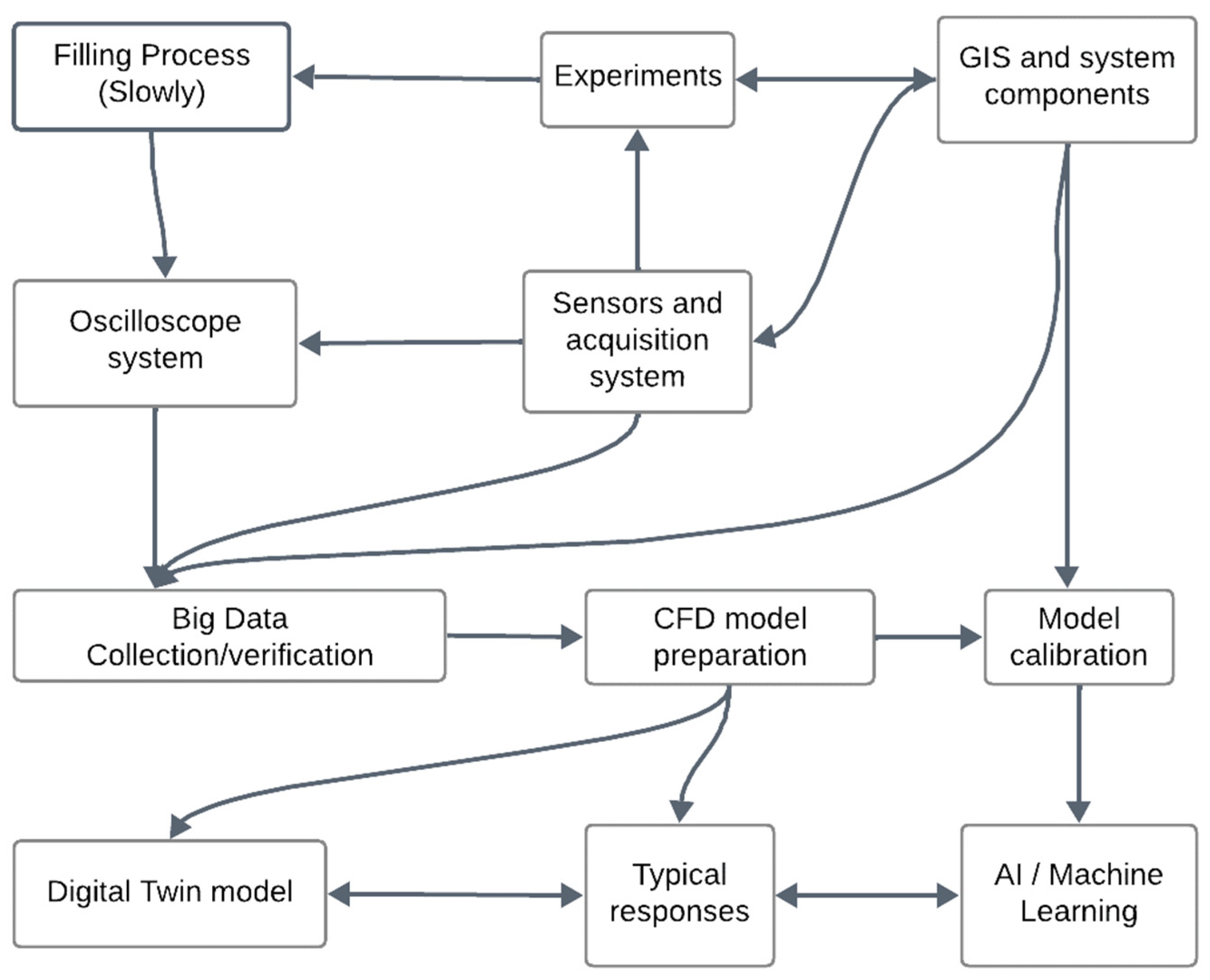
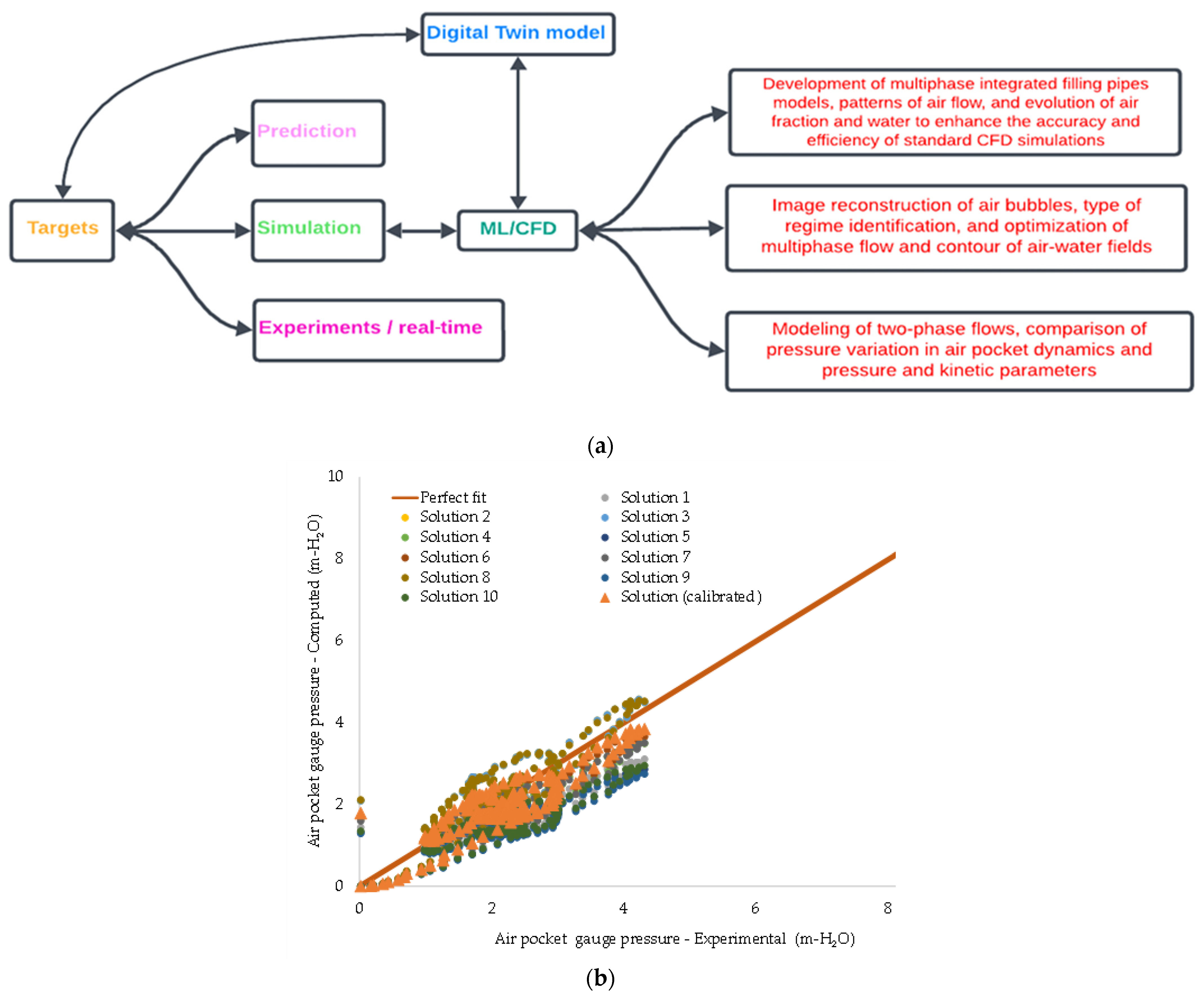
2.1. Digital Twin

This section details the development of the proposed Digital Twin applied to filling operations. Figure 1 illustrates the key components of the proposed model for filling maneuvers.

Filling operations can be carried out by the recommendations provided by the AWWA, which advise that these processes should be performed as slowly as possible [25]. The big data platform relates various components. The positioning of system elements pertains to pipes, junctions, valves, reservoirs, and hydraulic devices, which must be located using Geographical System Information (GIS). Sensors measure key hydraulic and thermodynamic parameters within water distribution systems. Pressure transducers (sensors) must be installed based on the behavior of transient events, with their placement determined by the required frequency. These sensors should be positioned near air valves. The design of maneuvers in regulating valves—whether manual, automatic, or electro-pneumatic—must be planned to prevent pipeline ruptures. Additionally, flow meters should be installed along water pipelines to monitor changes in water velocity over time. An electromagnetic flow meter or Ultrasonic Doppler Velocimetry can be selected depending on the required frequency. An oscilloscope system should be configured to translate hydraulic and thermodynamic variables into electrical signals. An air-water interface can be captured using cameras for transparent pipes. A trigger can be used as an electrical strategy to synchronize the different devices to start all measurements simultaneously. In this sense, the Internet of Things (IoT) is essential during this stage. Subsequently, a 3D CFD model must be implemented to simulate critical scenarios, such as small air pockets trapped in water installations. Currently, computational times present a challenge during the simulation phase. Implementing such a model involves defining the water infrastructure geometry, analyzing the sensitivity of a selected mesh, choosing a turbulence model and its associated numerical resolution scheme, establishing initial and boundary conditions, and executing an appropriate visualization process. In this context, the parameters of a 3D CFD model must be calibrated using experimental measurements to ensure the model is suitable for predicting filling operations. Once a reliable 3D CFD model is established, various scenarios can be simulated to analyze the behavior of filling processes under different initial pressures and air pocket sizes.

The proposed Digital Twin integrates a big data platform, a 3D CFD model, and artificial intelligence techniques (see Figure 1).

2.2. Big Data Platform

This study developed the big data platform\considering an experimental facility at the Hydraulic Laboratory of the Instituto Superior Técnico of the University of Lisbon. The facility consists of a pipeline with an inner diameter of 0.0514 m and a total length of 7.3 m. The pipeline has two branches: a left branch segmented by a horizontal and diagonal part ($L_{l,h}$ and $L_{l,d}$ with lengths of 2.05 m and 1.5 m, respectively) and a right branch segmented in branches $L_{r,d}$ and $L_{r,h}$ with lengths of 1.5 m and 1.85 m, respectively, as shown in Figure 2.

The air pocket pressure pulses were recorded employing the pressure transducer with S-10 WIKA from Germany, which is suitable for values up to 25 bar. This sensor has an analog signal with an electric current of 4 to 20 mA.

Real-time data analysis considered a ball valve closed at the end of the $L_{r,h}$. An electro-pneumatic ball valve guarantees a water inflow from the hydro-pneumatic tank located at the end of $L_{l,h}$, and an air valve located at the upper end of the hydraulic system was used to ensure adequate air expulsion. The analysis defines an initial air pocket with length $X_0$. A pressure transducer measures entrapped air’s pressure oscillations at the hydraulic system’s highest point. Air valve ARI S050 with an inner diameter ($d_0$) of 3.175 mm was used during the tests. This air valve can expel air at a rate of 80 m³/s, assuming a differential pressure of 8 bar. The real-time data involves water movement from the hydro-pneumatic tank to the pipeline using an initial pressure ($p_0$).

An electro-pneumatic ball valve was configured during the real-time data analysis for all tests from the Georg Fischer (+GF) company (Schaffhausen, Switzerland). It works with an electrical signal to activate the opening maneuver. The model 546 DN63-DN50 was employed in this research, with a pressure range varying from 5.6 to 7.0 bar. The electro-pneumatic ball valve opens for 0.20 s to generate the inflow from the hydro-pneumatic tank and the pipe filling. Once amplified, the signals are captured with a PicoScope model 3424. This device processes the air pocket pressure signals, converts them into digital form, filters out any noise, and records the data on a computer.

During filling, the air valve guarantees the expelling of the entrapped air, so the water column subsequently occupies the hydraulic installation. To represent different hydraulic scenarios, six tests were performed using various values of hydro-pneumatic pressure ($p_0$) and $X_0$. Hydro-pneumatic pressure varying from 20 to 50 kPa was used during the experimental stage. The hydraulic installation is at rest at the start of the transient event. The event is initiated by the opening of the electro-pneumatic ball valve, with six tests previously configured to generate different air pocket pressure patterns. Initial conditions were established considering pipeline conditions that must be conducted by water utilities, where the air pocket size needs to be filled by the water phase. This research is suitable for representing the assessment suggested by the AWWA in terms of water velocities and pressure variations [25].

Table 1. Initial conditions of experimental tests.

Test No.	${\mathit{p}}_0$ (kPa)	${\mathit{X}}_0$ (m)
1	20	0.46
2	20	0.96
3	20	1.36
4	50	0.46
5	50	0.96
6	50	1.36

shows the initial conditions of the tests.

3. Digital Twin—CFD Model

A three-dimensional computational fluid dynamic (CFD) model based on the PVoF method is developed to understand the entrapment and expelling of air. The air-water interaction in the CFD model considers hydraulic and thermodynamic assumptions: (i) two fluids (liquid and gas) were considered compressible fluids with non-homogeneous temperatures and immiscible, and (ii) roughness and water surface tension effects ($F_s$) were considered due to the significant ratio between absolute roughness ($K_s$) and pipe diameter ($D$). Appendix A shows the governing equations of the 3D CFD model.

3.1. Numerical Approach

The numerical approach to rapid hydraulic transients in pipelines is solved through second-order numerical schemes based on the Gauss linear upwind scheme due to the quick convergence to the numerical solution and the guarantee of temporal stability, especially regarding pressure, flux velocity, and turbulence. On the other hand, temperature is solved using a first-order numerical scheme of Gauss Upwind to optimize the solution time and prioritize the numerical solution of flow parameters (pressure and velocity). On the other hand, the Pressure-Implicit with Splitting of Operators (PISO) algorithm is used to solve the equations. This iterative algorithm efficiently handles the coupling between the pressure and velocity fields by splitting the pressure and velocity updates into separate steps, which favors the reduction of computational costs, and is suitable for these scenarios associated with transient flows and is commonly used in the modeling of flows in complex geometries and with frequent turbulent phenomena.

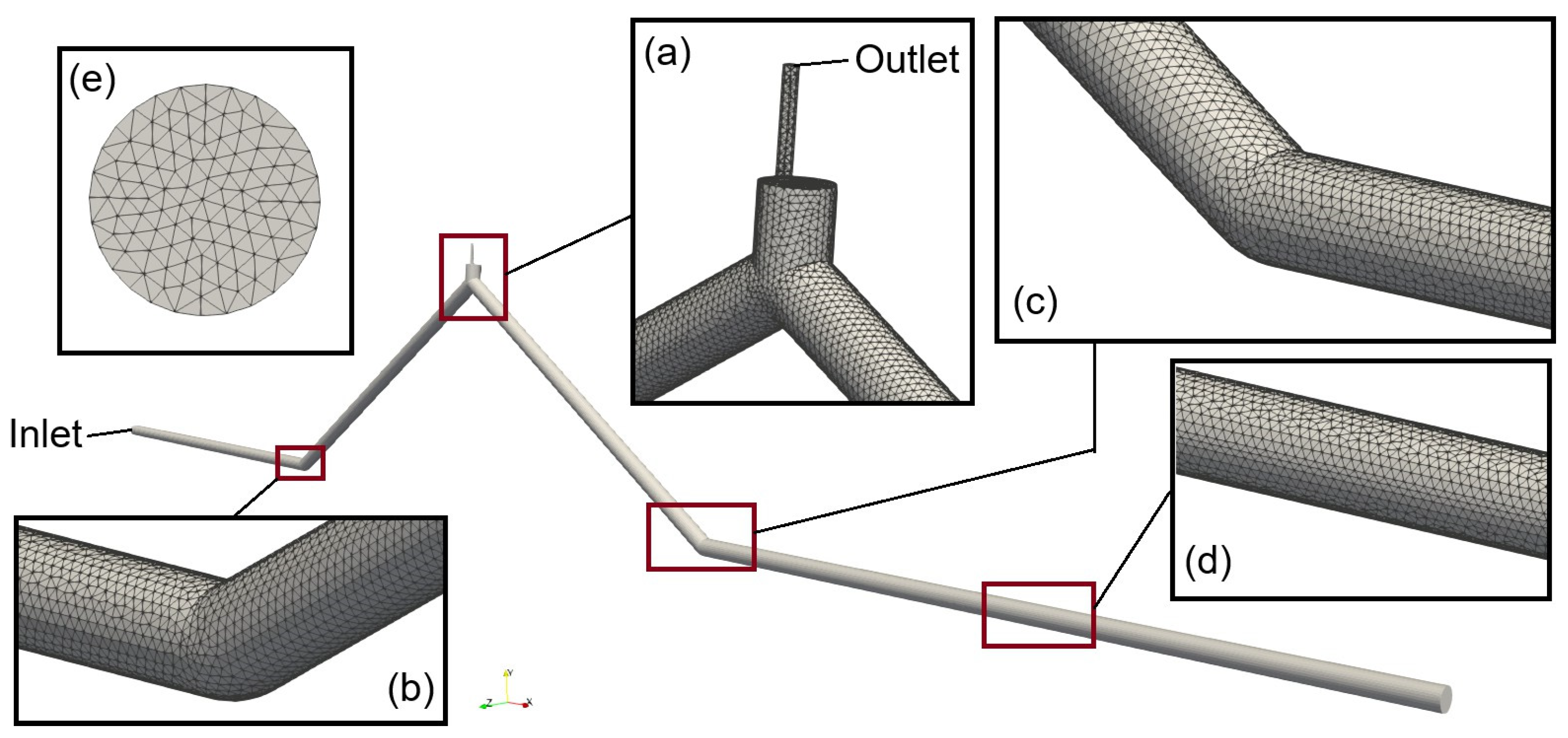
3.2. Geometry and Mesh

The irregular pipeline and the air valve are represented using a three-dimensional geometry composed of a longitudinal pipe of 6.9 m in length from the electro-pneumatic ball valve to the closed ball valve. The pipe has a diameter of 51.4 mm. Certain assumptions were considered to represent the irregular pipe in this study:

• The electro-pneumatic valve opens from the instant t = 0.0 s, and the effect of the opening is negligible.
• The ball valve in the experimental setup’s right sector is closed. Therefore, this element needs to be addressed in the geometry of the CFD model.
• The effect of the air valve is represented by a small pipe with a nominal diameter of one inch (1″) and an orifice with a diameter of 3.175 mm, corresponding to the discharge orifice of the S050 air valve.

The geometry is discretized into unstructured cells, with a maximum cell size of 0.005 m, ensuring a detailed representation of the flow domain. In particular, the region around the air valve section is further refined, with a maximum cell size reduced to 0.001 m, as shown in Figure 3. This mesh configuration comprises 330,793 cells, all of which are tetrahedral. The cell number selection process was based on the mesh independence analysis performed by the authors in previous investigations [26]. The number of cells selected reflects an acceptable mesh resolution suitable for capturing the complexities of flow phenomena within the pipeline at the experimental scale. The sensitivity analysis was performed, showing that the number of cells is independent of pressure patterns, which favors using this number of cells [26]. Moreover, choosing a fine mesh facilitates the physical analysis that governs the expulsion of air through the air valve S050.

3.3. Boundary Conditions

In the three-dimensional CFD model, boundary conditions are applied to different regions within the computational domain. The domain walls were characterized by a fixed flux pressure condition, representing a specified pressure boundary condition to account for the known pressure conditions at this pipe surface. Additionally, a no-slip condition was implemented for the velocity at the walls, assuming that the fluid velocity at the walls is zero. For the outlet boundary (air-release zone), a total pressure condition was applied to ensure that the outflow conditions adequately accounted for the atmospheric pressure ($p_{atm}$ = 101,325 Pa). In the same boundary, a pressure inlet-outlet velocity condition was enforced for velocity in the function of an atmospheric pressure condition. Moreover, the inlet boundary is defined with a total pressure determined by the absolute pressure ($p_{atm}+p_0$), reflecting the pressure of water inflow. On the other hand, a pressure inlet-outlet velocity condition for velocity dependent on the inlet pressure and the phase fraction condition at the inlet is defined by ${\alpha }_w$ = 1.0, which indicates a water inflow. The temperature conditions were set with a zero gradient at the walls and inlet boundaries, maintaining a constant temperature gradient. In contrast, an inlet-outlet ($I-O$) condition was imposed at the outlet to facilitate the flow of thermal energy.

3.4. Computational Process

The computational process of the CFD model is conducted using the compressibleInterFoam solver within the OpenFOAM v2102. The simulation is initiated from the initial time $t_0$ = 0 until $t$ = 2.0 s. To ensure temporal accuracy, a minimal time step of $1\times {10}^{-10}$ s was adopted, while a maximum time step of $5\times {10}^{-4}$ s was enforced to balance computational efficiency with solution stability. From the maximum and minimum time step values, the software automatically adjusts the time step according to the physical process occurring in the modeling, which depends on the maximum velocity presented in the model and is also controlled by a maximum Courant number of 0.9. During model processing, it was observed that the solution to the variables reached the numerical solution in 1 or 2 iterations.

4. Analysis of Results and Discussion

This section shows different methods of 3D CFD model validation. Air pocket pressure patterns provided reliable information, which is contained in the big data platform. These pulses are compared using numerical data from the 3D CFD model. In addition, the dynamic behavior of the air-water interface obtained from the CFD model contours is compared with the movement captured on video frames during the laboratory procedure.

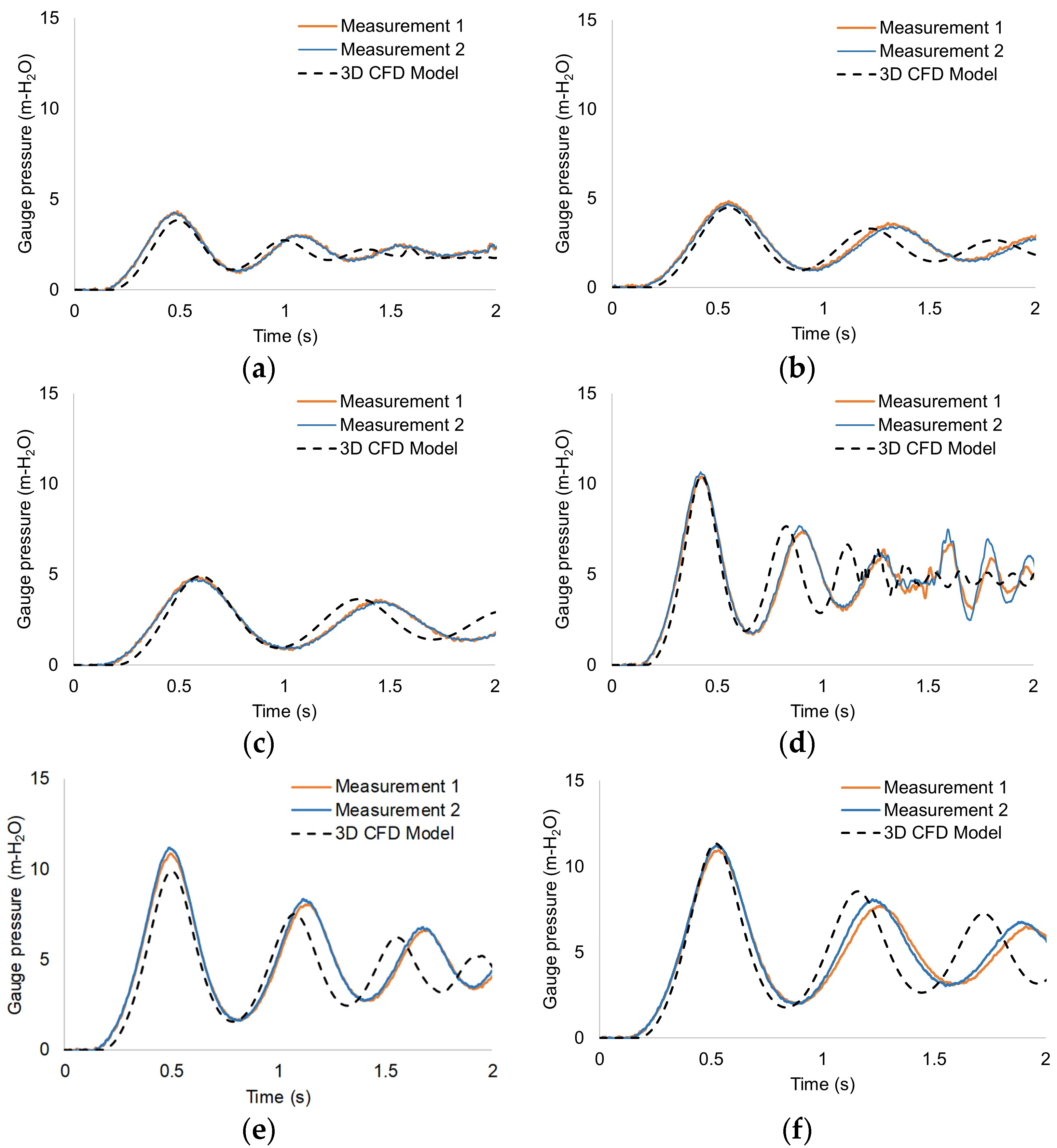
4.1. Numerical Validation of CFD Model

Six tests are performed in the laboratory with the initial conditions defined in Table 1. The pressure patterns obtained by the 3D CFD model are compared with the measurements obtained from the big data platform taken in the laboratory, as shown in Figure 4.

The CFD model oscillations generally present a similar trend to the pressure measurements regarding the number of peaks, adequately predicting the first pressure peak in all tests, which is usually the most critical peak in transient filling processes with trapped air.

Tests 1, 2, and 3 are performed at an inlet gauge pressure of 20 kPa. Thus, the maximum gauge pressure peaks ranged between 4.2 and 4.8 m-H₂O, while Tests 4, 5, and 6 were performed at a pressure of 50 kPa, thus generating gauge pressure peaks between 10.5 and 10.8 m-H₂O. In Tests 1 and 4, where the initial air pocket was 0.46 m long, it is possible to observe oscillations given by origin different from the compression and expansion processes of the air pocket. This is because the water column reaches the upper end of the pipe, thus generating pressure oscillations given as a product of the collision of the water column at the upper end of the network before t = 2.00 s. This phenomenon is not shown in Tests 2, 3, 5, and 6 because the filling processes in these cases exceed the 2 s in the laboratory measurements.

In order to validate the accuracy of this model, the maximum pressure values are compared with those measured in the tests from the calculation of the relative error, using the formula $ϵ=\left|{\displaystyle \frac{p_{max,exp}-p_{max,CFD}}{p_{max,exp}}}\right|$, where $p_{max,exp}$ = maximum pressure in an experimental test, and $p_{max,CFD}$ = maximum pressure in a CFD scenario.

Table 2. Root Mean Square Error for maximum pressure.

Test No.	${\mathit{p}}_{\mathit{m}\mathit{a}\mathit{x},\mathit{e}\mathit{x}\mathit{p}}$ (m)	${\mathit{p}}_{\mathit{m}\mathit{a}\mathit{x},\mathit{C}\mathit{F}\mathit{D}}$ (m)	$\mathit{ϵ}$ (%)
1	4.29	3.84	10.0%
2	4.67	4.48	4.1%
3	4.71	4.78	2.4%
4	10.53	10.42	1.0%
5	11.05	9.90	10.0%
6	11.34	11.10	2.2%

shows the values of $ϵ$ for each test, highlighting a good agreement of peak values of air pocket pressure of experimental and numerical conditions due to the values being less or equal to 10%, making this limit value appropriate for numerical resolution in CFD. Errors between CFD and experimental values may be related to the accuracy in capturing complex transient phenomena such as air-water interaction in these filling processes. In addition, minor variations in the initial experimental conditions may influence the observed differences.

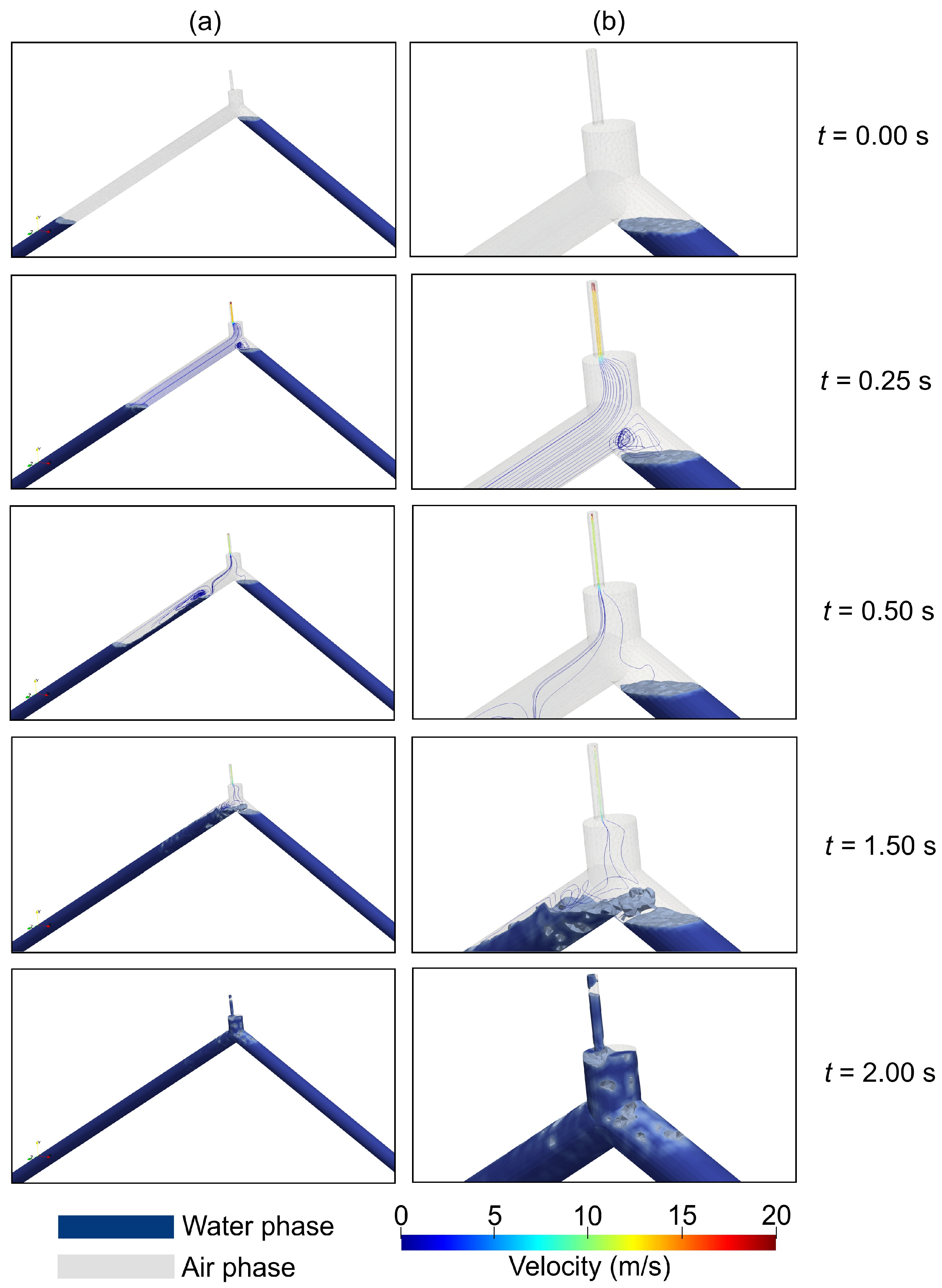
4.2. Validation of Air-Water Interaction

During the laboratory tests, a video was recorded of the filling process of Test 5, and images were processed using Machine Learning (ML) (Figure 5), which is used to validate the 3D CFD model. The frames are a recorded sample of observed data obtained from the six tests performed in the laboratory. ML and data science drive a transformative shift in hydraulic engineering, offering significant advantages in understanding and predicting complex hydraulic phenomena during the filling process. ML is a powerful tool that complements incomplete domain-specific knowledge typically used in conventional experimental and computational methods. ML provides flexible techniques for developing robust predictive models, eliminating values outside the pattern operating zone by identifying hidden patterns and mechanisms in data sets. This capability is particularly advantageous in hydraulic transients and filling processes, where traditional methods may fall short.

For instance, ML can enhance multiphase flow modeling by improving closure models for air expulsion, turbulence stresses, pulsation events, and backflow occurrence, thereby increasing the accuracy and efficiency of CFD simulations. Additionally, ML can assist in image reconstruction, regime identification, parameter prediction, and optimizing flow and air-dragging fields. Despite its many strengths, ML also presents challenges, such as the need for high-quality data and the risk of overfitting. Still, its application is to accelerate advancements in hydraulic systems, providing new opportunities for research and innovation in this field. Figure 6 represents five time instances of the filling process associated with Test 5. Frames from the post-processing of the 3D CFD model and video frames are used in this analysis.

These CFD and experiment images are compared, and the sequence of events occurring in the filling process is analyzed, which is also described below:

• t = 0.00 s: At that instant, the pipe contains an initial air pocket at atmospheric conditions, and the water column is at rest since the filling process has not yet started.
• t = 0.25 s: The water column at the left branch gradually rises due to the hydro-pneumatic tank pumping, and the air-water interface starts to exhibit a different shape. In addition, the location of the air-water interface in the frame of the CFD model and the experimental one is similar.
• t = 0.50 s: The water column returns slightly in the opposite direction of flow, and the air-water interface collapses, generating a transition from pressurized flow to free surface flow, which occurs in the CFD model and the experiment facility.
• t = 1.54 s: The water column has reached the upper end of the pipe, thus displacing part of the air volume that the air valve S050 has expelled. At this stage, a moderate mixing of air bubbles with the water phase begins to be generated, evident in the CFD model frame and the experiment’s video frame.
• t = 2.00 s: Much of the pipe’s air volume is expelled at this experiment stage. In that sense, the pipe is almost entirely occupied by water. Small bubbles are observed due to the mixing of air and water at the high point of the pipe and are evident experimentally and numerically through the contours of the CFD model.

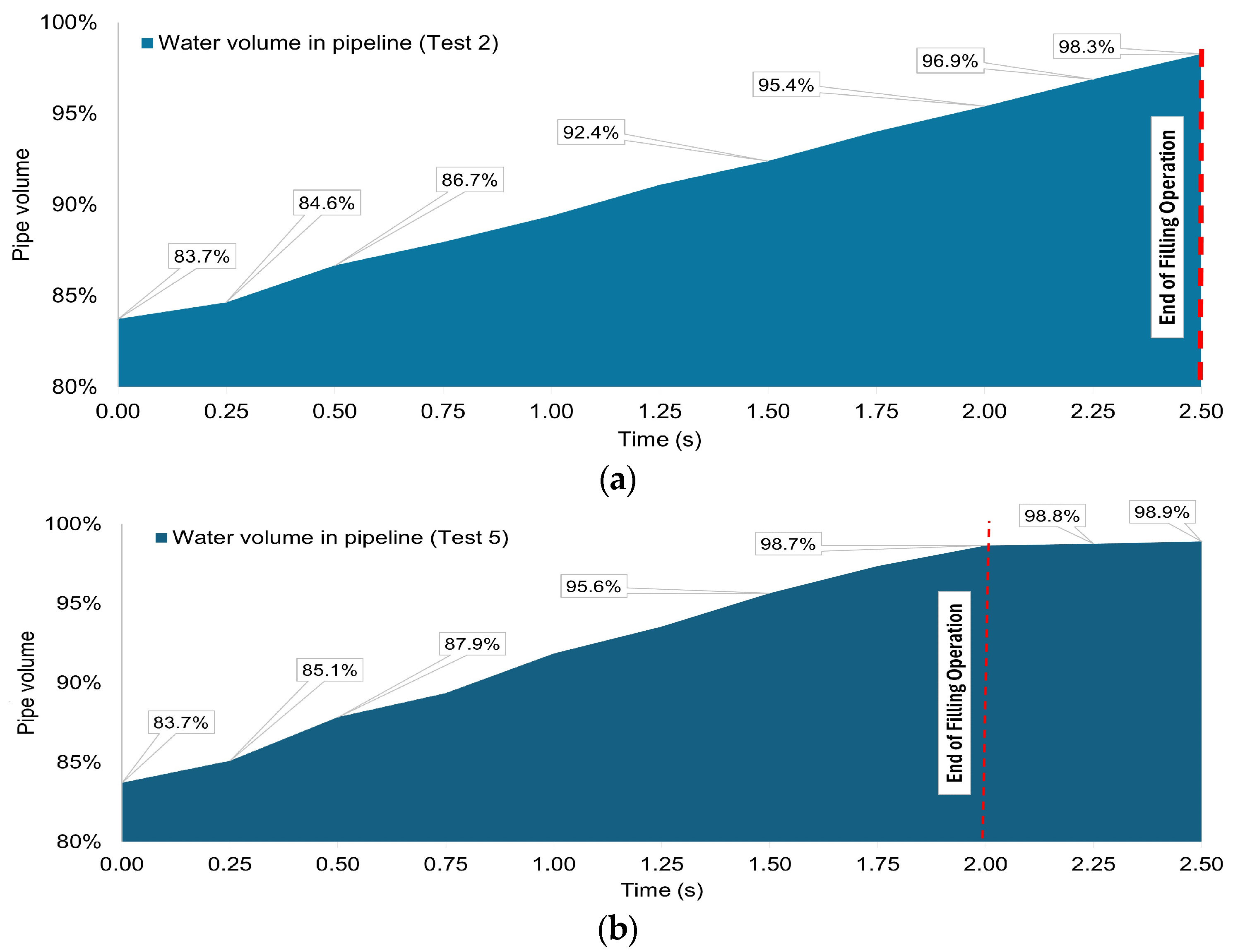
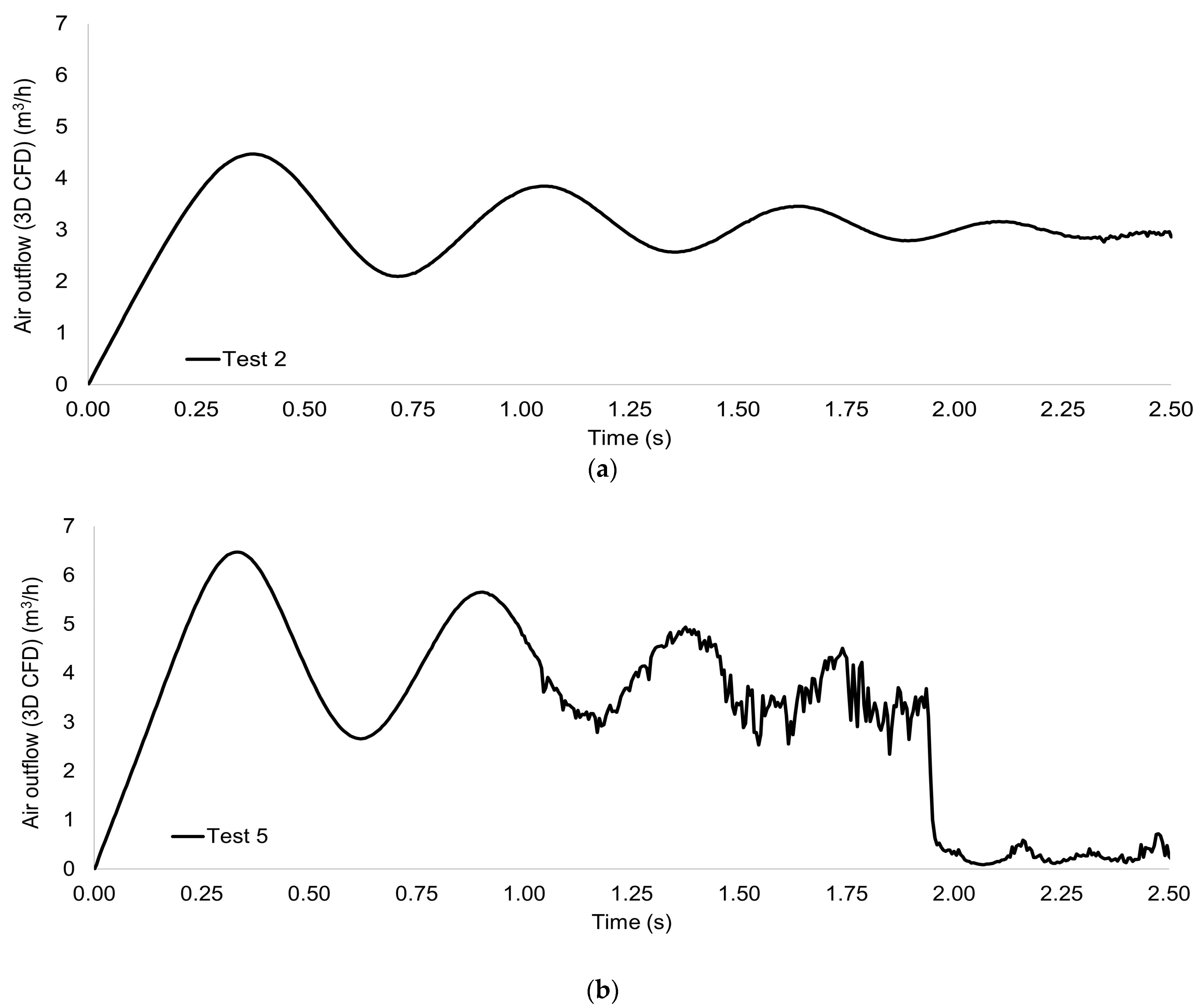
4.3. Dynamic of Air Expulsion from Pipelines

This section emphasizes analyzing the behavior of the air expelled through the air valve S050 from the volume of water inside the pipe. Figure 7 shows the evolution of the volume of water inside the pipe during the filling process, which is related to the amount of air expelled from the hydraulic system.

In Test 2 (Figure 7a), the initial air pocket is $X_{0,l}$ = 0.96 m. i.e., 83.7% of the pipe volume is occupied by water. When the filling process starts, the water occupies 84.6% of the total volume of the pipe at t = 0.25 s. After that, the water volume fraction of the pipeline increases to 86.7% at t = 0.50 s. Subsequently, the pipe’s water percentage amounts to 92.4% and 95.4% at t = 1.50 s and t = 2.00 s, respectively. At t = 2.25 s, the water filling process is still occurring at 96.9% of the water over the volume of the pipe, and finally, at t = 2.50 s, the water reaches 98.3% of the volume of the pipe. At this moment, the water column has reached the upper zone of the pipe, thus completing the filling process. In general, the amount of water in the pipeline gradually increased due to the controlled pressure applied to the water column and the controlled operation of the air valve S050 to expel the trapped air.

In the case of Test 5 (Figure 7b), the initial air pocket is also 0.96 m. At t = 0.25 s, the water column occupies 85.1% of the total volume of the pipe, which is noticeable when the water column rises without generating a collapse of the air-water interface (see Figure 5). At t = 0.50 s, the water column still influences the air outflow out of the pipe, although this undergoes a backflow (see Figure 6). In this instant, the water occupies 87.9% of the volumetric capacity of the pipe. At t = 1.50 s, the water column has expelled a significant percentage of the trapped air. At this instant, the volume of water available is 95.6%. At the same time, at t = 2.00 s, the pipe is almost entirely occupied by water, with a fraction of the total pipe volume equal to 98.7%, leaving 1.3% of air accumulated at the upper end of the pipe. This amount of air contained in the pipe at t = 2.00 s is demonstrated in experience, where it is stated that pressurized water flow in pipes occasionally has a certain amount of air equivalent to 2.7% on average, according to Lauchlan et al. (2005) [7]. At this instant, the filling process is completed. However, there is a slight oscillation of water volume between t = 2.00 s and t = 2.50 s, going from 98.7% to 98.9%, which is not a significant difference.

Figure 8 shows the evolution of air outflow over time through the S050 air valve from the 3D CFD model during the filling process in Tests 2 and 5. Figure 8b shows the air outflow behavior in Test 2. When the filling process starts due to the hydro-pneumatic tank pumping, the air is expelled, generating a first flow peak with the value of 4.47 m³/h at t = 0.38 s. Subsequently, the air outflow rate decreases gradually to 2.10 m³/h at t = 0.72 s. This decrease in air outflow occurs because the trapped air pocket accumulates compression energy, which is subsequently released and generates a backflow of water in the pipeline, thus leading to a transient dissipation of the airflow. Afterward, a new increase in the air outflow is generated, with a peak value of 3.85 m³/h at t = 1.06 s, and subsequently, a second valley value is generated at t = 1.33 s with a flow of 2.59 m³/h. This oscillatory behavior of the air outflow is maintained over time, dissipating the amplitude of the oscillations, being that the air outflow converges to a rate of 2.92 m³/h.

Figure 8b shows the air outflow behavior. After the hydro-pneumatic tank is actuated to supply water to the pipeline, the airflow rate increases to 6.24 m³/h at t = 0.29 s. After that, the air outflow rate decreases gradually to 2.66 m³/h at t = 0.62 s. A second peak is generated with a value of 5.65 m³/h at t = 0.9 s, and subsequently, a second valley value is generated at t = 1.17 s with a flow of 2.79 m³/h. In these time instants mentioned, the flow oscillations are stable; this is because the air-water interface had low susceptibility to violent mixing processes between both fluids; this is evidenced by the time instants of t = 0.25 s and t = 0.50 s from Figure 5. On the other hand, after the time instant t = 1.25 s, the airflow pattern presents secondary oscillations in the central air discharge flow oscillation pattern until an instant of time t = 1.94 s. These secondary oscillations occur due to the mixing of air and water in the upper area of the hydraulic system (air valve area S050), which is visible at t = 1.54 s and t = 2.00 s from Figure 5. After the instant t = 2.00 s (when the filling process ends), a minimum discharge flow with an average value of 0.27 m³/h is present.

In post-processing tools, CFD models show streamlines resulting from the movement of fluids, in this case, air, which is a highly compressible fluid. Knowledge of the trajectory of the streamlines over the hydraulic system helps to identify whether the geometrical conditions of the air valve’s exhaust orifice influence the efficiency of air exhaust processes.

Figure 9 shows the evolution of the trajectory of the streamlines of the air expelled in Test 5 at five (5) time instants, which are analyzed below:

• t = 0.00 s: There are no air streamlines at this instant due to the hydraulic system being at rest.
• t = 0.25 s: At this instant, air streamlines parallel the pipe axis with a velocity between 0 and 5 m/s. These are located between the initial air-water interface, up to the upper end of the pipe, where there is a vorticity at the corner. On the other hand, the air streamlines increase in velocity at the end of the air valve to values between 10 and 15 m/s. At the discharge orifice, the velocity increases to a value higher than 20 m/s, according to the observed contours.
• t = 0.50 s: The air streamlines in the air valve zone decrease in velocity magnitude due to the number of streamlines, while vortices occur in the air pocket as a result of the transient event, in which the air pocket releases energy after compressing in the first oscillation. Velocity contours are the same at time instant t = 0.25 s.
• t = 1.50 s: At this instant, the air streamlines are chaotically distributed in the upper zone of the pipe without being traced in the air valve structure. At this time, the airflow velocity is less than 5 m/s.
• t = 2.00 s: The filling process ends, so it is not easy to visualize the tracing of the air streamlines.

To bear in mind, the proposed Digital Twin can be applied to real-world pipeline systems by addressing several key aspects: (i) 3D CFD simulations, which can take months depending on available computational power, invariably require high-performance resources; (ii) real-time data acquisition using pressure transducers distributed along the pipelines is essential to validate the Digital Twin’s results; and (iii) water utilities should utilize cloud computing to meet the demands associated with modeling large-scale hydraulic systems.

This research can be utilized to understand ruptures in pressurized hydraulic installations during filling operations in complex systems containing multiple air pockets. Water utilities often replace pipe materials; however, a deeper understanding could help reduce maintenance costs by enabling the appropriate operation of regulating valves and establishing an air valve maintenance plan. Additionally, it can aid in minimizing water supply interruptions for repairs, particularly in systems prone to frequent ruptures.

5. Conclusions

This study applied real-time data and CFD modeling to examine air-release dynamics during irregular pipe-filling processes. By integrating a Digital Twin platform, 3D CFD simulations, and Artificial Intelligence (AI) technologies, the research identified critical aspects of trapped air management, such as the air pocket extension, air outflow patterns through valves, the evolution of filling, and the aerodynamic behavior of expelled air. These insights significantly improve water conveyance systems’ efficiency, reliability, and safety, particularly in complex pipeline networks. The results show that the 3D CFD model, calibrated with real-time experimental data, accurately represents air-release dynamics, offering a reliable tool for analyzing the performance of air valves under various conditions. ML can provide flexible techniques to facilitate the conceptual development of new robust predictive models for multiphase flows: (i) development of multiphase integrated models filling pipes, patterns of air flow, and evolution of air fraction and water to enhance the accuracy and efficiency of standard CFD simulations; (ii) image reconstruction of air bubbles, type of regime identification, and optimization of multiphase flow and contour of air-water fields; and (iii) modeling of two-phase flows, comparison of pressure variation in air pocket dynamics and pressure and kinetic parameters.

Key findings regarding the integration of Digital Twins platforms and CFD modeling are highlighted in this context.

• This study contributes to developing an integrated system for real-time monitoring of pipeline operations. It includes the three-dimensional representation from computational fluid dynamics tools that allows the identification of the air-water interaction from this study scenario and the detailed evolution of fluid parameters such as pressure, velocity–velocity, and temperature spatially and temporally.
• This study represents a breakthrough in the simulation of the filling process with entrapped air and air valves in three dimensions, going beyond 2D CFD simulation that relied on discharge orifices to approximate air ejection effects.
• The integration of CFD models and Digital Twins has several limitations: data sources, interpretability of results, robustness of the integrated model, phenomenon complexity, machine learning efficiency, and extrapolation of results. However, this research also faced several challenges and opportunities: analysis of results, discussion, and future directions.

Therefore, future research should focus on several areas, including studying trapped air management in different branches of water distribution networks and the interaction between hydraulic systems and the mechanical features of air valves, such as the valve body, float, and closing mechanisms. Integrating Geographic Information Systems (GIS), Digital Twin technology, and AI in detecting anomalies, like abnormal pressure patterns, is more used to enhance system safety. Additionally, improving real-time data acquisition through smart sensors and further refining mathematical models will help address current limitations in field applications, providing more reliable and efficient management of transient events in water conveyance systems.

References

- Ramos, H.M.; Fuertes-Miquel, V.S.; Tasca, E.; Coronado-Hernández, O.E.; Besharat, M.; Zhou, L.; Karney, B. Concerning Dynamic Effects in Pipe Systems with Two-Phase Flows: Pressure Surges, Cavitation, and Ventilation. Water 2022, 14, 2376. [Google Scholar] [CrossRef]
- John, H.B., Jr.; Dechant, D.A. Current Proposed Changes to AWWA M11 Steel Pipe: A Guide for Design and Installation. In Proceedings of the Pipelines 2014: From Underground to the Forefront of Innovation and Sustainability, Portland, OR, USA, 3–6 August 2014; pp. 2221–2228. [Google Scholar] [CrossRef]
- Boulos, P.F.; Karney, B.W.; Wood, D.J.; Lingireddy, S. Hydraulic Transient Guidelines for Protecting Water Distribution Systems. J. Am. Water Work. Assoc. 2005, 97, 111–124. [Google Scholar] [CrossRef]
- Crabtree, A.; Oliphant, K. Resistance of PE4710 Piping to Pressure Surge Events in Force Main Applications. 2012. Available online: https://conduitcalc.plasticpipe.org/pdf/resistance-of-pe4710-piping-to-pressure-surge-evnets-in-force-main-applications.pdf (accessed on 10 September 2024).
- Hussam, F.; Tarek, Z. Hierarchical Fuzzy Expert System for Risk of Failure of Water Mains. J. Pipeline Syst. Eng. Pr. 2010, 1, 53–62. [Google Scholar] [CrossRef]
- Ramezani, L.; Karney, B.; Malekpour, A. Encouraging Effective Air Management in Water Pipelines: A Critical Review. J. Water Resour. Plan. Manag. 2016, 142, 4016055. [Google Scholar] [CrossRef]
- Lauchlan, C.; Escarameia, M.; May, R.; Burrows, R.; Gahan, C. Air in Pipelines—A Literature Review. 2005. Available online: https://eprints.hrwallingford.com/551/1/SR649.pdf (accessed on 10 September 2024).
- Zhou, L.; Cao, Y.; Karney, B.; Bergant, A.; Tijsseling, A.S.; Liu, D.; Wang, P. Expulsion of Entrapped Air in a Rapidly Filling Horizontal Pipe. J. Hydraul. Eng. 2020, 146, 4020047. [Google Scholar] [CrossRef]
- Malekpour, A.; Shahroodi, A. What Is a Safe Filling Velocity in Water and Wastewater Pipelines? In Proceedings of the Pipelines 2023, San Antonio, TX, USA, 12–16 August 2023; pp. 301–312. [Google Scholar] [CrossRef]
- Tasca, E.S.A.; Karney, B. Improved Air Valve Selection through Better Device Characterization and Modeling. J. Hydraul. Eng. 2023, 149, 4023019. [Google Scholar] [CrossRef]
- Ramezani, L.; Karney, B.; Malekpour, A. The Challenge of Air Valves: A Selective Critical Literature Review. J. Water Resour. Plan. Manag. 2015, 141, 4015017. [Google Scholar] [CrossRef]
- García-Todolí, S.; Iglesias-Rey, P.L.; Mora-Meliá, D.; Martínez-Solano, F.J.; Fuertes-Miquel, V.S. Computational Determination of Air Valves Capacity Using CFD Techniques. Water 2018, 10, 1433. [Google Scholar] [CrossRef]
- Zhou, F.; Hicks, F.E.; Steffler, P.M. Transient Flow in a Rapidly Filling Horizontal Pipe Containing Trapped Air. J. Hydraul. Eng. 2002, 128, 625–634. [Google Scholar] [CrossRef]
- De Martino, G.; Fontana, N.; Giugni, M. Transient Flow Caused by Air Expulsion through an Orifice. J. Hydraul. Eng. 2008, 134, 1395–1399. [Google Scholar] [CrossRef]
- Carlos, M.; Arregui, F.J.; Cabrera, E.; Palau, C.V. Understanding Air Release through Air Valves. J. Hydraul. Eng. 2011, 137, 461–469. [Google Scholar] [CrossRef]
- Fuertes-Miquel, V.S.; López-Jiménez, P.A.; Martínez-Solano, F.J.; López-Patiño, G. Numerical Modelling of Pipelines with Air Pockets and Air Valves. Can. J. Civ. Eng. 2016, 43, 1052–1061. [Google Scholar] [CrossRef]
- Coronado-Hernández, Ó.E.; Besharat, M.; Fuertes-Miquel, V.S.; Ramos, H.M. Effect of a Commercial Air Valve on the Rapid Filling of a Single Pipeline: A Numerical and Experimental Analysis. Water 2019, 11, 1814. [Google Scholar] [CrossRef]
- Zhou, L.; Pan, T.; Wang, H.; Liu, D.; Wang, P. Rapid Air Expulsion through an Orifice in a Vertical Water Pipe. J. Hydraul. Res. 2019, 57, 307–317. [Google Scholar] [CrossRef]
- Romero, G.; Fuertes-Miquel, V.S.; Coronado-Hernández, Ó.E.; Ponz-Carcelén, R.; Biel-Sanchis, F. Analysis of Hydraulic Transients during Pipeline Filling Processes with Air Valves in Large-Scale Installations. Urban. Water J. 2020, 17, 568–575. [Google Scholar] [CrossRef]
- Li, L.; Zhu, D.Z.; Huang, B. Analysis of Pressure Transient Following Rapid Filling of a Vented Horizontal Pipe. Water 2018, 10, 1698. [Google Scholar] [CrossRef]
- Chan, S.N.; Cong, J.; Lee, J.H.W. 3D Numerical Modeling of Geyser Formation by Release of Entrapped Air from Horizontal Pipe into Vertical Shaft. J. Hydraul. Eng. 2018, 144, 04017071. [Google Scholar] [CrossRef]
- Wang, J.; Vasconcelos, J.G. Investigation of Manhole Cover Displacement during Rapid Filling of Stormwater Systems. J. Hydraul. Eng. 2020, 146, 4020022. [Google Scholar] [CrossRef]
- Fang, H.; Zhou, L.; Cao, Y.; Cai, F.; Liu, D. 3D CFD Simulations of Air-Water Interaction in T-Junction Pipes of Urban Stormwater Drainage System. Urban. Water J. 2022, 19, 74–86. [Google Scholar] [CrossRef]
- Aguirre-Mendoza, A.M.; Paternina-Verona, D.A.; Oyuela, S.; Coronado-Hernández, O.E.; Besharat, M.; Fuertes-Miquel, V.S.; Iglesias-Rey, P.L.; Ramos, H.M. Effects of Orifice Sizes for Uncontrolled Filling Processes in Water Pipelines. Water 2022, 14, 888. [Google Scholar] [CrossRef]
- American Water Works Association (AWWA). Air-Release, Air/Vacuum, and Combination Air Valves: M51; American Water Works Association (AWWA): Denver, CO, USA, 2001; Volume 51. [Google Scholar]
- Paternina-Verona, D.A.; Coronado-Hernández, O.E.; Espinoza-Román, H.G.; Arrieta-Pastrana, A.; Tasca, E.; Fuertes-Miquel, V.S.; Ramos, H.M. Attenuation of Pipeline Filling Over-Pressures through Trapped Air. Urban. Water J. 2024, 21, 698–710. [Google Scholar] [CrossRef]
- Martins, N.M.C.; Delgado, J.N.; Ramos, H.M.; Covas, D.I.C. Maximum Transient Pressures in a Rapidly Filling Pipeline with Entrapped Air Using a CFD Model. J. Hydraul. Res. 2017, 55, 506–519. [Google Scholar] [CrossRef]