Abstract
One of the most basic issues in fluid mechanics is the description of flow in closed flows; more precisely, the calculation of pressure drops and the description of the flow form. Therefore, in this paper, the numerical simulation of the flow through the elbow was presented. This case was used to comprehensively describe the most important phenomena that should be taken into account during closed flows. The elbow was chosen as one of the most frequently used fittings in practice. The simulation was made with ANSYS Fluent, with the use of the turbulent model k-ω, SIMPLE simulation method, and at Reynolds number . The minor and major pressure loss were presented and discussed in the paper. The minor loss coefficient at the high Reynolds number was equal to around 0.2, which is close to the value of 0.22 used in engineering calculations. The influence of the Reynolds number on the shift of the stream separation point in the elbow was described. The secondary flow in the elbow was observed and the vortex structure was discussed and shown with the use of the Q-criterion (Q iso surface for level 0.005). This analysis allowed us to better visualize and describe the complex flow structure observed in the investigated case.
1. Introduction
The elbows are one of the most frequently used fittings in duct engineering installations. Examples of their application include in gaseous fuel supplies, exhaust installations, ventilation systems, technical gas installations, and many others. The flow through the elbow is also very complex. The widespread use and complexity of the flow make it an excellent facility for operational research and flow analysis, as it is used much more often than other types of fittings. The elbow is very often used as an example fitting for major and minor loss calculation [1,2], mass transfer [3,4], and multi-phase analyses [5,6,7].
Ono et al. [8] investigated the influence of the elbow curvature on the flow structure for high Reynolds numbers ( and ). They showed that the use of a large bending radius of the elbow significantly affects the flow separation at the outlet—the separation region in the long elbow is formed intermittently. They also described secondary flow in the outflow. A more complex description of the secondary flow was made by Sudo et al. [9]. They observed that secondary flow develops into a pair of vortices at a 30-degree angle (calculated from the inlet to the elbow). The secondary flow was observed even for a distance from the elbow equal to 10D, where D was the diameter of the channel. An analysis of the secondary flow was also undertaken by Röhrig et al. [10], Kim et al. [11], and others [12,13,14,15]. On the other hand, Patiño-Jaramillo et al. [16] analyzed flow through the tee joints for different configurations but only in 2D simulation without secondary flow analysis. Recently, research in the field of the numerical analysis of flow in elbows due to erosion occurring during pipeline operation has also been developing dynamically; see Sun et al. [17], Liu et al. [18], and Chen and Tan [19]. These investigations connect the flow structure with the shape of erosion occurring in pipelines.
The elbow is very often used in the analysis of the loss coefficient. dos Santos et al. [1] investigated the minor loss of elbow at different Reynolds numbers and proposed an equation describing this relationship. Smyk et al. [20] investigated minor and major loss coefficients for straight ducts and elbows for different duct diameters, elbow angles, and Reynolds numbers. They used different simulation models during the investigation. A similar investigation was also undertaken by Salehi et al. [21]. Lui et al. [22] proposed a procedure for predicting pressure loss coefficients based on the example of the tee. However, the simulation model was chosen based on the simulation of losses in the elbow. The interaction between two elbows and their impact on the flow field and losses was investigated by Sami and Ciu [23], Zmrhal and Schwarzer [24], and Weissenbrunner et al. [25]. All these studies were numerical. This is due to the search for a reliable method of determining local loss coefficients for fittings. Cheap methods that do not require time-consuming and expensive experimental research are also sought. All this research indicated the unreasonableness of treating the local loss coefficient as one value (in engineering practice).
The article presents the simulation of the flow in the elbow. The simulation was made for nine different Reynolds numbers in a range from 500 to 100,000 and the results were discussed due to the influence of the Reynolds number. The paper combines issues in the field of local losses and flow characteristics in the elbow, providing a broader context for understanding this basic but complex phenomenon. The paper paid particular attention to the hydraulic entry length that had to be maintained during the simulation, and the secondary flow was described in detail, through the use of a Q iso surface. Additionally, the impact of the Reynolds number on the angle of separation point in the elbow was discussed. For this reason, in the authors’ opinion, the work is a particularly extensive study of the described topic, which may constitute a springboard for a broader discussion and further description and the investigation of flows in closed channels.
2. Materials and Methods
The simulation of the flow through the elbow was made in ANSYS Fluent 2019 and the investigated model was presented in Figure 1. The diameter of the duct was equal to mm and the bending radius of the elbow was equal to mm. The length of the inlet duct was equal to and the outlet duct was . Steady simulation was used, and gravity was not taken into account. The turbulent model k-ω and SIMPLE simulation method were used. During all simulations, y+ values were below 1. The velocity inlet boundary condition was used on the inlet and the pressure outlet one on the outlet. The roughness of the wall was defined as 0 mm. Table 1 presents the parameters of the simulation.
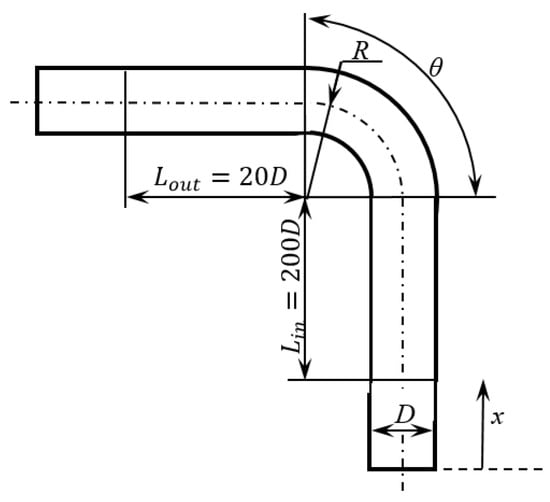
Figure 1.
Model of measuring system.

Table 1.
Parameters of simulation.
The Reynolds number was calculated as
where is the mean velocity, defined in Table 1 [m/s]. The simulation was made for water with density kg/m3 and kinematic viscosity m2/s. The Dean number was calculated as
Grid Independence
The first step of the simulation was an analysis of the grid independence. Figure 2 presents the dependence between the pressure drop and the number of elements (Figure 2a) and between the maximal velocity on the outlet and the number of elements (Figure 2b). Based on this dependence, selected mesh parameters corresponding to 5.26 million elements were chosen. It must be noted that the difference between the investigated parameters obtained for this and the best mesh was smaller than 1%.
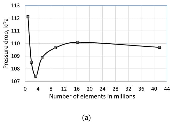
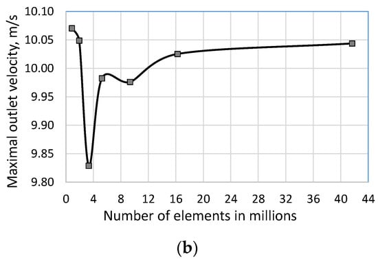
Figure 2.
The pressure drop (a) and maximal velocity on the outlet (b) depending on the number of elements at .
3. Results and Discussion
3.1. Hydrodynamic Entry Length and Head Loss
Figure 3 presents the profile of the ratio of centerline velocity () to mean velocity for different Reynolds numbers. This profile can be used to determine the hydrodynamic entry length [26,27]. Based on the ratio velocity profile presented in Figure 3, the entry length can be determined as in case of and as in case of , and generally the higher Reynolds number, the longer entry length (the length at which the velocity values in the axis stabilize). Additionally, at for , fluctuation can be observed in the ratio velocity, which was not observed for other Reynolds numbers. It is caused by the elbow. Therefore, the head pressure loss was calculated from for all investigated cases.
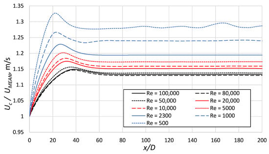
Figure 3.
The profile of the ratio of centerline velocity () to mean velocity () for different Reynolds numbers in the inlet duct.
Figure 3 shows that the ratio of centerline velocity to mean velocity decreased with the Reynolds number. This is a phenomenon that should be expected due to the flattening of the velocity profile with an increase in the Reynolds number [28,29,30]. The velocity ratio stabilized around the value of at .
The numerical major/head loss coefficient (called Darcy friction factor or Darcy–Weisbach friction factor) was calculated from the Darcy–Weisbach equation, as follows:
where is a static pressure drop in the inlet duct at a distance [Pa], and is the measuring length ( m). The theoretical value of the Darcy factor was calculated from Poiseuille’s equation (laminar flow, ) and Blasius’s equation (turbulent flow, ) [31] successively, as follows:
Figure 4 presents a comparison of the Darcy friction factor calculated based on the simulation for different Reynolds numbers, where the Reynolds number is presented in a logarithmic scale. The numerical and theoretical simulations were similar at a high Reynolds number . Additionally, Figure 4 presents the numerical Darcy friction factor calculated for the k-ω simulation by Smyk et al. [20]. The course of the curve obtained in [20] is more similar to the theoretical course, but the errors in the laminar range are similar to those in the presented simulation. It is worth noting that data from [20] were meant for eight different diameters, and the presented data are calculated for only one diameter of the duct.
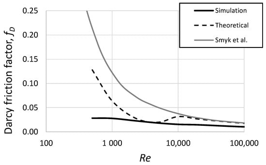
Figure 4.
The Darcy friction factor from the simulation, the theoretical one based on Equations (4) and (5), and the one from Smyk et al. [20].
The differences between the obtained and theoretical Darcy friction factors do not seem to be big. However, the smallest percentage difference between them was obtained at and was equal to 7.5%. The theoretical Darcy friction factor at was 12 times bigger than the numerical one. The analysis of the major pressure coefficient is not a goal of this paper and is useful only for calculating the minor/local pressure coefficient. For this reason, the calculated and theoretical coefficients do not need to be equal in value. Smyk et al. [20] showed that the best turbulence model for the calculation of the Darcy friction factor is the Spalart–Allamars turbulence model. It must be noted that Poiseuille’s and Blasius’s equations were experimentally designed. However, their theoretical justification was given by George Stokes. The problem of calculating the Darcy friction factor was discussed in more detail in [32,33,34].
3.2. Minor Loss Coefficient
To calculate the local loss factor, two steps were performed. These were (1) the calculation of the static pressure drop between three points: the inlet duct at a distance and the outlet of the outlet duct; (2) a reduction in the obtained pressure by major pressure losses calculated with the use of numerical Darcy friction factor (presented in Figure 4), and calculation of the minor loss coefficient based on the following equation:
where is a pressure drop calculated in the second step [Pa]. The calculated minor loss coefficient is presented in Figure 5. Additionally, the value was marked on the chart. The value was taken from [35]. This book is one of the most commonly used (in Poland) for designing and calculating ventilation systems.
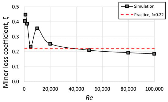
Figure 5.
The simulated minor loss coefficient vs. the Reynolds number. The value was marked with the red dashed line.
The highest value of the minor loss coefficient was obtained at . The local maximum was also observed at . The decrease in the minor loss coefficient for was also observed in other papers [1,21,36]. The increase in the pressure loss in the area of transition from laminar to turbulent flow was observed in [12].
3.3. Flow Analysis
The elbow and other types of fittings can cause velocity distribution, not only in a plane of the flow (YZ plane in investigated case, see Figure 6) but also in the perpendicular plane (XY plane in the investigated case, see Figure 6), observed as secondary flow [9,11,14,37]. The secondary flow is most often observed with the use of proper orthogonal decomposition (POD) of the velocity field [37,38]. The secondary flow is related to the appearance of a velocity component perpendicular to the flow plane (the velocity component parallel to the X-axis; see Figure 6 and Figure 7). The line of the velocity was measured was shown in Figure 7. All lines were parallel to the X–axis.
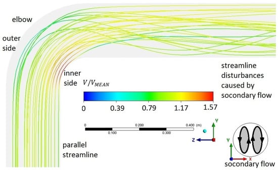
Figure 6.
The streamline in the analyzed system at .
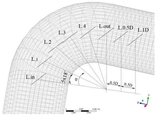
Figure 7.
The location of measurement line—the L.in line is located at the beginning of the elbow and the L.out line at the end of the elbow.
The u velocity was also analyzed at distances and before the elbow, but even at the velocity was equal to zero at a distance before the elbow. At a distance before the elbow, the u velocity was at least 100 times lower than for the other lines tested. Such low values are negligible; therefore, the analysis of the u component was started from the L.in line located at the beginning of the elbow (Figure 7). The above observations are consistent with experimental studies by Sudo et al. [9].
Figure 8 presents the radial profile of the velocity on the measurement line presented in Figure 7 at different Reynold numbers. The profiles were presented as function, where is a distance from the duct axis. The velocity was equal to zero in at all investigated Reynolds numbers and for all measurement lines. The higher the Reynolds number, the higher the value of velocity. The velocity profile was generally sinusoidal; however, at lines L.2 and L.3 (Figure 8c,d) a distribution of the profile was observed. Particular attention should be paid to the change in the direction of the velocity vector near the elbow wall at line L.2 (Figure 8c). This phenomenon was observed at a distance at , and the distance decreased as the Reynolds number increased. It was not observed at . The different direction of the velocity indicates the presence of secondary flow in the elbow. It can be seen better in the presentation of the tangential velocity vector. Figure 9 shows the tangential velocity vector in the plane passing through line L.2. The change in the direction of the velocity vector was not visible in this case. But the shape of the vector clearly indicates the formation of vortex structures in this elbow. These structures, called secondary flow, were also observed at . According to the classification of the secondary flow patterns by Sudo et al. [9], this type of the vortex structure should be classified as the first type of secondary flow. This structure was observed for all investigated Dean and Reynolds numbers (Table 1).
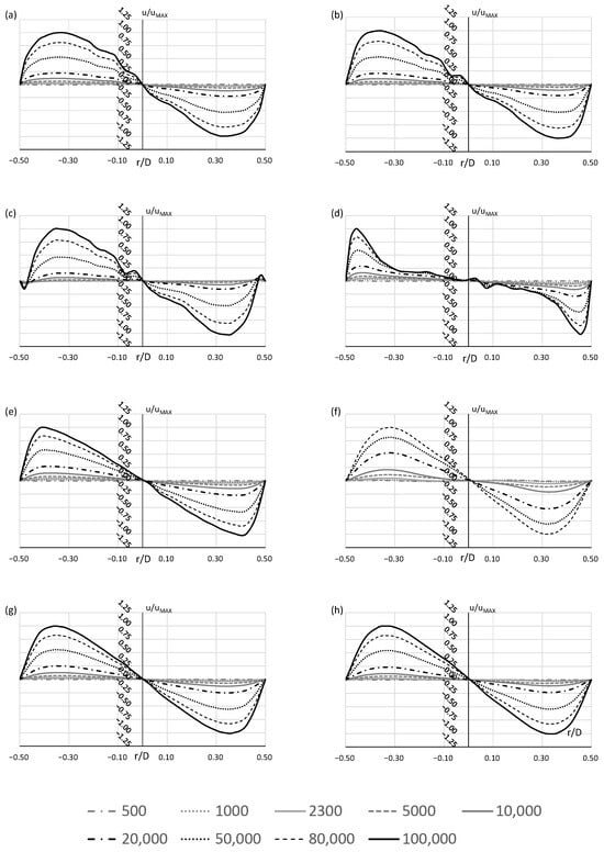
Figure 8.
The radial profile of the velocity on the L.in (a), L.1 (b), L.2 (c), L.3 (d), L.4 (e), L.out (f), L.0.5D (g), and L.1D (h).
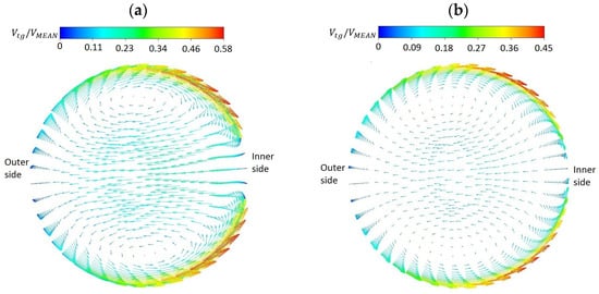
Figure 9.
The tangential velocity () vector in a plane perpendicular to the elbow and passing through line L.2 at (a) and (b).
Kalpakli et al. [38] observed that the change in the secondary flow (tangential velocity vector) depends on the location of measurements in the elbow and outer pipe. Röhrig et al. [10] carried out the same experiment numerically and expanded Kalpakli et al. [38]’s investigation. The change in the tangential velocity vector is caused mainly by the separation of the flow and the formation of a vortex structure behind the elbow. Figure 10 presents the dependence between the separation angle α (the angle determines the location of the separation point of the stream on the inner wall of the elbow) and the Reynolds number. The separation angle is presented in Figure 7. Generally, the higher the Reynolds number, the further the separation point is moved towards the outlet. This behavior is an effect of the pressure distribution in the duct and the Coanda effect [39,40].
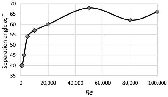
Figure 10.
The separation point location vs. the Reynolds number.
The separation angle increased with the increase in the Reynolds number (Figure 10). Firstly, it was linear in a laminar and transitional flow region (). At a high Reynolds number (), the value of the separation angle oscillated around . Figure 11 presents the velocity vectors in a ZY plane (see Figure 6 and Figure 7) at three different Reynolds number values. The separation point is visible as a sudden decrease in the velocity value near the inner wall of the elbow. Behind the separation point, the pressure decreases and the vortex structure is generated. In general, the higher the Reynolds number, the larger the vortex structure. It is very visible when comparing the velocity vector in the elbow at (Figure 11a) and (Figure 11c). The vortex structure visible in Figure 11 creates a flow dead zone. The size of the flow dead zone generally depends on the location of the separation point. It is important to pay attention to the stabilization of the value of the separation angle (Figure 10) and the minor loss coefficient (Figure 5) at a high Reynolds number (). Of course, the minor loss coefficient also depends on other vortex structures and losses generated in an elbow as a secondary flow (Figure 9).
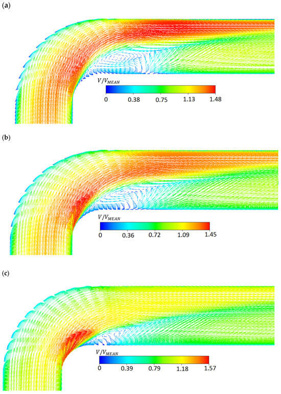
Figure 11.
The velocity vector in elbow and outlet duct at (a), (b), and (c).
The secondary flow and the vortex structure visible in Figure 11 overlap and create a relatively complex vortex structure inside the elbow. One of the methods for vortex identification is a Q-criterion [41]. Figure 12 shows the Q iso surface for the level equal to 0.005. The vortex shape indicates how much secondary flow contributes to the flow in the elbow. Additionally, the size of the structure shows that the impact of the secondary flow decreases with an increase in the Reynolds number. The characteristic structure of the vortex shown in Figure 11 could be observed along the entire length of the outlet channel in all investigated cases.
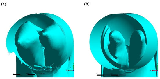
Figure 12.
Q iso surface for level 0.005 on the outlet of the elbow at (a) and (b).
The occurrence of vortices presented by the Q iso surface in Figure 12 is one of the reasons for the pressure loss in the elbow–vortex structures, which dissipates the energy of the flow. One of the methods for extinguishing them is the use of straighteners, before, after, or during the fittings [42,43,44]. However, the operation of straighteners is based on the use of appropriate elements to extinguish turbulence due to increased local pressure losses or physically preventing the formation of vortex structures [45]. Therefore, the quenching of vortices may be energetically unjustified, even though, with an increase in the Reynolds number, they appear faster and have greater intensity (understood in this case as Q being a function of strain rate tensor and vorticity tensor). However, the vortex structure can affect measurements that take place immediately behind chokes such as elbows [25].
4. Conclusions
The paper deals with the simulation of the flow in the elbow. The turbulent k-ω model and SIMPLE simulation method were used and the Reynolds number was analyzed in a range from to . Based on the presented discussion and analysis, the following conclusions can be drawn:
- The k-ω model can be used to calculate head pressure loss. However, the Darcy friction factor was similar to the theoretical value only in the case of the high Reynolds number ().
- The calculated minor loss coefficient depends on the Reynolds number. The calculated value of the minor loss coefficient was similar to the engineering/literature value at . The minor loss coefficient should be better investigated for Reynolds numbers .
- The secondary flow was observed in all investigated cases. It was observed also by the analysis of the velocity profile.
- The separation point location depends on the Reynolds number and is stabilized for , similar to the minor loss coefficient. The analysis of the velocity vectors showed the flow dead zone behind the elbow. The flow dead zones were bigger the lower the Reynolds number.
- The Q-criterion vortex identification method showed two vortex structures. They were the result of overlapping of the main flow and the secondary flow. The impact of the secondary flow decreased with the Reynolds number increasing.
Author Contributions
Conceptualization, software, investigation, resources, data curation, writing—original draft preparation, supervision, funding acquisition, visualization, project administration, E.S.; methodology, validation, formal analysis, E.S. and M.S. (Michał Stopel); writing—review and editing, M.S. (Michał Stopel) and M.S. (Mikołaj Szyca). All authors have read and agreed to the published version of the manuscript.
Funding
This research received no external funding.
Data Availability Statement
All data generated or used during the study are available from the corresponding author upon request.
Conflicts of Interest
The authors declare no conflicts of interest.
References
- dos Santos, A.P.P.; Andrade, C.R.; Zaparoli, E.L. CFD Prediction of the Round Elbow Fitting Loss Coefficient. Int. J. Mech. Mechatron. Eng. 2014, 8, 743–747. [Google Scholar]
- Smyk, E.; Mrozik, D.; Wawrzyniak, S.; Peszyński, K. Tabular air deflector in ventilation ducts. In Proceedings of the 23rd International Conference Engineering Mechanics, Svratka, Czech Republic, 15–18 May 2017; pp. 882–885. [Google Scholar]
- Gallegos-Muñoz, A.; Uzárraga Rodríguez, N.C.; Belman Flores, J.M.; Rangel Hernández, V.H. Analysis of effect caused by fitting in the measurements of flow in air conditioning system. Appl. Therm. Eng. 2012, 33–34, 227–236. [Google Scholar] [CrossRef]
- Wang, J.; Shirazi, S.A. CFD based correlation for mass transfer coefficient in elbows. Int. J. Heat Mass Transf. 2001, 44, 1817–1822. [Google Scholar] [CrossRef]
- Spedding, P.L.; Benard, E.; Crawford, N.M. Fluid flow through a vertical to horizontal 90° elbow bend III three phase flow. Exp. Therm. Fluid Sci. 2008, 32, 827–843. [Google Scholar] [CrossRef][Green Version]
- Zahedi, R.; Babaee Rad, A. Numerical and experimental simulation of gas-liquid two-phase flow in 90-degree elbow. Alex. Eng. J. 2022, 61, 2536–2550. [Google Scholar] [CrossRef]
- Cao, X.; Zhang, P.; Li, X.; Li, Z.; Zhang, Q.; Bian, J. Experimental and numerical study on the flow characteristics of slug flow in a horizontal elbow. J. Pipeline Sci. Eng. 2022, 2, 100076. [Google Scholar] [CrossRef]
- Ono, A.; Kimura, N.; Kamide, H.; Tobita, A. Influence of elbow curvature on flow structure at elbow outlet under high Reynolds number condition. Nucl. Eng. Des. 2011, 241, 4409–4419. [Google Scholar] [CrossRef]
- Sudo, K.; Sumida, M.; Hibara, H. Experimental investigation on turbulent flow through a circular-sectioned 180° bend. Exp. Fluids 2000, 28, 51–57. [Google Scholar] [CrossRef]
- Röhrig, R.; Jakirlić, S.; Tropea, C. Comparative computational study of turbulent flow in a 90° pipe elbow. Int. J. Heat Fluid Flow 2015, 55, 120–131. [Google Scholar] [CrossRef]
- Kim, J.; Yadav, M.; Kim, S. Characteristics of secondary flow induced by 90-degree elbow in turbulent pipe flow. Eng. Appl. Comput. Fluid Mech. 2014, 8, 229–239. [Google Scholar] [CrossRef]
- Spedding, P.L.; Benard, E.; Mcnally, G.M. Fluid Flow through 90 Degree Bends. Dev. Chem. Eng. Miner. Process. 2010, 12, 107–128. [Google Scholar] [CrossRef]
- Dutta, P.; Nandi, N. Effect of Reynolds number and curvature ratio on single phase turbulent flow in pipe bends. Mech. Mech. Eng. 2015, 19, 5–16. [Google Scholar] [CrossRef]
- Jarrahi, M.; Castelain, C.; Peerhossaini, H. Secondary flow patterns and mixing in laminar pulsating flow through a curved pipe. Exp. Fluids 2011, 50, 1539–1558. [Google Scholar] [CrossRef]
- Rup, K.; Sarna, P. Analysis of turbulent flow through a square-sectioned duct with installed 90-degree elbow. Flow Meas. Instrum. 2011, 22, 383–391. [Google Scholar] [CrossRef]
- Patiño-Jaramillo, G.A.; Iglesias, I.; Vera, M. Laminar flow and pressure loss in planar Tee joints: Numerical simulations and flow analysis. Eur. J. Mech. B/Fluids 2022, 92, 75–89. [Google Scholar] [CrossRef]
- Sun, Q.L.; Xia, L.; Deng, L.; Wang, J.G.; Wang, G.L.; Feng, D. Experimental and Numerical Simulation Analyses of Elbow Erosion in Surface Process of Deepwater Gas Well Testing. J. Fail. Anal. Prev. 2024, 24, 202–215. [Google Scholar] [CrossRef]
- Liu, E.B.; Huang, S.; Tian, D.C.; Shi, L.M.; Peng, S.B.; Zheng, H. Experimental and numerical simulation study on the erosion behavior of the elbow of gathering pipeline in shale gas field. Pet. Sci. 2024, 21, 1257–1274. [Google Scholar] [CrossRef]
- Chen, M.; Tan, L. An improved method combined modified drag model and modified erosion model based on LES for solid-liquid multiphase flow and erosion with application in a 90° elbow. Wear 2024, 538–539, 205214. [Google Scholar] [CrossRef]
- Smyk, E.; Mrozik, D.; Łukasz, O.; Peszyński, K. Numerical simulation of minor losses coefficient on the example of elbows. EPJ Web Conf. 2018, 180, 02093. [Google Scholar] [CrossRef][Green Version]
- Salehi, M.; Sleiti, A.K.; Idem, S. Study to identify computational fluid dynamics models for use in determining HVAC duct fitting loss coefficients. Sci. Technol. Built Environ. 2017, 23, 181–191. [Google Scholar] [CrossRef]
- Liu, W.; Long, Z.; Chen, Q. A procedure for predicting pressure loss coefficients of duct fittings using computational fluid dynamics (RP-1493). HVAC R Res. 2012, 18, 1168–1181. [Google Scholar] [CrossRef]
- Sami, S.; Cui, J. Numerical study of pressure losses in close-coupled fittings. HVAC&R Res. 2004, 10, 539–552. [Google Scholar] [CrossRef]
- Zmrhal, V.; Schwarzer, J. Numerical simulation of local loss coefficients of ventilation duct fittings. In Proceedings of the Eleventh International IBPSA Conference, Glasgow, Scotland, 27–30 July 2009; pp. 1761–1766. [Google Scholar]
- Weissenbrunner, A.; Ekat, A.; Straka, M.; Schmelter, S. A virtual flow meter downstream of various elbow configurations. Metrologia 2023, 60, 5. [Google Scholar] [CrossRef]
- Durst, F.; Ray, S.; Ünsal, B.; Bayoumi, O.A. The development lengths of laminar pipe and channel flows. J. Fluids Eng. Trans. ASME 2005, 127, 1154–1160. [Google Scholar] [CrossRef]
- Kahramanoglu, E.; Sezen, S.; Bayraktar, S. Computational fluid dynamics analyses on the hydrodynamic entry length in internal flows. Pamukkale Univ. J. Eng. Sci. 2017, 23, 372–377. [Google Scholar] [CrossRef]
- Grossmann, S.; Lohse, D. Curvature effects on the velocity profile in turbulent pipe flow. Eur. Phys. J. E 2017, 40, 7–12. [Google Scholar] [CrossRef] [PubMed]
- Bariya, H.G.; Patel, M.P. On the Solution of Blasius Boundary Layer Equations of Prandtl-Eyring Fluid Flow Past a Stretching Sheet. Indian J. Sci. Technol. 2024, 17, 1237–1244. [Google Scholar] [CrossRef]
- Wang, Y.; Zhang, Z. Asymptotic behavior of the steady Prandtl equation. Math. Ann. 2023, 387, 1289–1331. [Google Scholar] [CrossRef]
- Cengel, Y.A.; Cimbala, J.M. Fluid Mechanics: Fundamentals and Applications; Mc Graw-Hill, Higher Education: New York, NY, USA, 2006. [Google Scholar]
- Turgut, O.E.; Asker, M.; Çoban, M.T. A review of non iterative friction factor correlations for the calculation of pressure drop in pipes. Bitlis Eren Univ. J. Sci. Technol. 2014, 4, 1–8. [Google Scholar] [CrossRef]
- Vatankhah, A.R. Approximate Analytical Solutions for the Colebrook Equation. J. Hydraul. Eng. 2018, 144, 1–8. [Google Scholar] [CrossRef]
- Kiijarvi, J. Darcy Friction Factor Formulae in Turbulent Pipe Flow. Lunowa Fluid Mech. Pap. 2011, 110727, 1–11. [Google Scholar]
- Hendiger, J.; Ziętek, P.; Chlidzinska, M. Wentylacja i klimatyzacja. Materiały pomocnicze do projektowania (From Polish: Ventilation and Air Conditioning. Support Materials for Design); Venture Industries Sp. z.o.o.: Warszawa, Poland, 2013. [Google Scholar]
- Dutta, P.; Nandi, N. Study on pressure drop characteristics of single phase turbulent flow in pipe bend for high reynolds number. ARPN J. Eng. Appl. Sci. 2015, 10, 2221–2226. [Google Scholar]
- Glenn, A.L.; Bulusu, K.V.; Shu, F.; Plesniak, M.W. Secondary flow structures under stent-induced perturbations for cardiovascular flow in a curved artery model. Int. J. Heat Fluid Flow 2012, 35, 76–83. [Google Scholar] [CrossRef]
- Kalpakli, A.; Örlü, R.; Alfredsson, P.H. Vortical patterns in turbulent flow downstream a 90° curved pipe at high Womersley numbers. Int. J. Heat Fluid Flow 2013, 44, 692–699. [Google Scholar] [CrossRef]
- Valeriu, D. A New Mathematical Model for Coandă Effect Velocity Approximation. Incas Bull. 2012, 4, 85–92. [Google Scholar] [CrossRef]
- Dumitrache, A.; Frunzulica, F.; Ionescu, T.C. Mathematical Modelling and Numerical Investigations on the Coanda Effect. In Nonlinearity, Bifurcation and Chaos-Theory and Applications; Hagedorn, P., Awrejcewicz, J., Eds.; InTech: London, UK, 2012; pp. 101–132. [Google Scholar]
- Jeong, J.; Hussain, F. On the identification of a vortex. J. Fluid Mech. 1995, 285, 69–94. [Google Scholar] [CrossRef]
- Peszynski, K.; Tesař, V.; Kuliś, E. Evaluation of linear losses in ventilation ducts with a rounded rectangle cross-section. MATEC Web Conf. 2019, 302, 01021. [Google Scholar] [CrossRef][Green Version]
- Jurga, A.P.; Janocha, M.J.; Ong, M.C.; Yin, G. Numerical Investigations of Turbulent Flow Through a 90-Degree Pipe Bend and Honeycomb Straightener. J. Fluids Eng. 2024, 146, 021307. [Google Scholar] [CrossRef]
- Puspitasari, D.; Pramadhony, P.; Ellyanie, E.; Marwani, M. The effects of flow straightener inclination on distribution of flue gas flow. AIP Conf. Proc. 2018, 2001, 060002. [Google Scholar]
- Scheiman, J. Comparison of Experimental and Theoretical Turbulence Reduction Characteristics for Screens, Honeycomb, and Honeycomb-Screen Combinations; NASA Technical Paper; NASA: Washington, DC, USA, 1981. [Google Scholar]
Disclaimer/Publisher’s Note: The statements, opinions and data contained in all publications are solely those of the individual author(s) and contributor(s) and not of MDPI and/or the editor(s). MDPI and/or the editor(s) disclaim responsibility for any injury to people or property resulting from any ideas, methods, instructions or products referred to in the content. |
© 2024 by the authors. Licensee MDPI, Basel, Switzerland. This article is an open access article distributed under the terms and conditions of the Creative Commons Attribution (CC BY) license (https://creativecommons.org/licenses/by/4.0/).