Article

Approximate Solutions of the Boussinesq Equation for Horizontal Unconfined Aquifers During Pure Drainage Phase

Department of Civil Engineering and Geomatics, Cyprus University of Technology, Limassol 3036, Cyprus
*
Author to whom correspondence should be addressed.
Water 2024, 16(20), 2984; https://doi.org/10.3390/w16202984
Submission received: 27 August 2024 / Revised: 4 October 2024 / Accepted: 8 October 2024 / Published: 19 October 2024
(This article belongs to the Section Hydrology)

Abstract

:
In this work, conceptual approximations of the Boussinesq equation were introduced and analyzed, resulting into a very accurate and well-applicable model for horizontal unconfined aquifers during the pure drainage phase, without any recharge and zero-inflow conditions. The model was constructed by employing a variety of methods that included wave solution, variable separation, and series expansion, and its analysis and performance against the Boussinesq equation, at early and later times, providing fruitful insights enlightening the main mechanisms and physical characteristics of the drainage phase. The modeled non-linear forms were finally linearized, concluding with explicit analytical expressions that accurately incorporated most of the basic characteristics regarding the evolution of the water table and the outflow from the exact Boussinesq equation under different initial conditions. The endeavors of this work can be utilized for theoretical and modeling purposes related to this problem.

1. Introduction

Understanding groundwater dynamics is crucial in hydraulic engineering in order to describe and analyze fluid flow through aquifers, whether they are horizontal or inclined. The Boussinesq equation [1,2] effectively models water flow in aquifers. The equation is derived using the classical Dupuit–Forchheimer assumptions [3,4,5], considering a two-dimensional, horizontally infinite, homogeneous aquifer under fully saturated conditions, involving horizontal flow with a negligible vertical component.
In reality, vertical flow often varies with depth due to factors like aquifer heterogeneity, anisotropy, and varying hydraulic conductivity, which affect the accuracy of the model. Additionally, real aquifers are finite, and ignoring boundary effects can lead to inaccurate predictions of groundwater behavior, particularly near the edge. However, such assumptions provide a simplified framework for analyzing groundwater flow under idealized conditions and facilitate the derivation of analytical solutions. The primary challenge in obtaining solutions is the equation’s nonlinearity. This arises from dimensional considerations and the assumption that vertical flow can be treated as homogeneous, making the fluid flux proportional to the free-surface height times the hydraulic gradient.
Due to the dynamic nature of the Boussinesq equation in various groundwater flow applications, extensive theoretical and experimental efforts have been made [6,7,8,9,10,11,12,13,14,15,16,17,18,19,20,21,22] to find both exact and approximate solutions tailored to specific scenarios, after defining the mathematical problem with appropriate boundary conditions. New models of the Boussinesq equation for water flow accurately simulate groundwater dynamics, offering analytical and numerical solutions for unconfined aquifers during drainage, with applications in hydrology and engineering. According to [23], water motion involves the flow of water molecules, driven by forces like gravity, pressure gradients, and wind through various mediums such as rivers, oceans, aquifers, and atmospheric systems.
Finding solutions to the Boussinesq equation is vital, and the pursuit of both analytical and approximate solutions remains an active research area. When feasible, approximate solutions offer the benefits of simplicity and ease of mathematical treatment, making them straightforward to implement. Although not entirely capturing the complexity of real cases in the field, such solutions offer clear insights into the main mechanisms and physics behind the problem and can be used as building blocks in understanding and modeling more complicated and representative examples. This is precisely the motivation driving this research.
Specifically, in this study, naturally applicable approximations were employed to construct a new model for subsurface flow over a horizontal bed during the pure drainage phase of unconfined aquifers under steady hydraulic conditions. Both numerical and analytical solutions were derived, and it was shown that they accurately captured the main nonlinear Boussinesq equation characteristics, decoding changes in the water table shape and depth, while handling different initial conditions in contrast to former works. In the problem at hand, the case may start with a full aquifer at a steady state, created after uniform recharge at a constant rate [24,25,26]. Stopping recharging leads to the transition to the pure drainage phase, which is the topic of the present work.
Similarly, drainage can be conceptually forced by applying a sudden drawdown, which is a well-studied case for a semi-infinite aquifer, modified to approximate the finite one [7,27,28,29,30,31,32,33] in a quite cumbersome way that obscures the main mechanisms driving the flow. Furthermore, such solutions, although very accurate, are tailored to a very specific initial condition, not allowing for their general applicability.
In general, for the case of groundwater flowing in a horizontal finite aquifer at a zero-recharge rate, the solution of the equation can be obtained by assuming separation of the variables [2,7], which is actually an exact asymptotic solution of the horizontal aquifer recession phase for late times. However, the intermediate behavior of the flow and its response to different initial conditions is not well-known, which is where this work is trying to offer some insights.
The rest of this paper is organized as follows. In Section 2, we present the derivation of the Boussinesq equation during drainage and proceed with dimensionless formulation and analysis of the late-time behavior of the drainage phase, linking the findings with the series expansion of the profile. In Section 3, we introduce and analyze a novel approximate model for solving the drainage phase for several different initializations using the methods of wave approximation and series expansion. The model encapsulates the main characteristics of Boussinesq and satisfies mass-balance, furthermore, after linearization, it allows for a clear, explicit, and very accurate approximation. Finally, in Section 4, the major results of this work are summarized and emphasized.

2. Pure Drainage Flow in Horizontal Unconfined Aquifers

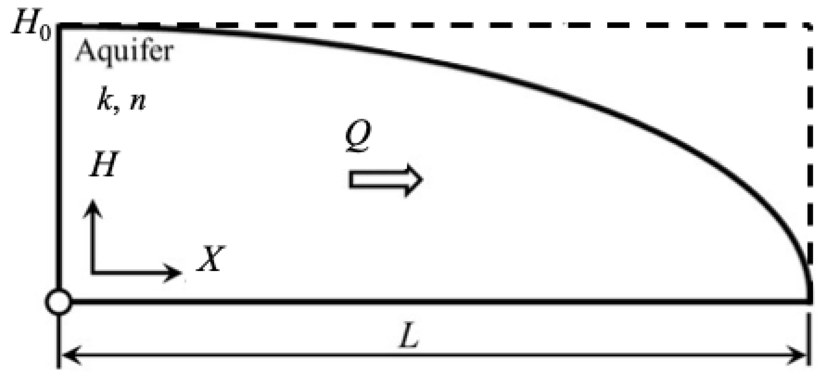
This section aims to summarize the established results to ensure that our presentation is comprehensive. The formulation to be presented incorporates common assumptions in aquifer modeling, particularly addressing the drainage phase of a horizontal aquifer following the recharge period. The aquifer was assumed to be horizontal with a flat bed and uniform hydraulic properties both spatially and temporally. We also assumed uniform and constant hydraulic conductivity (k) and drainable porosity (n) throughout the aquifer, with the resulting flow considered saturated and effectively one-dimensional. The impermeable bottom of the aquifer was also assumed to be flat and horizontal. A diagram of the aquifer with its main characteristics is provided in Figure 1.
The Dupuit–Forchheimer approximation links the flow per unit of width for each time instant, T, and for each position, X, over the application area (0 < X < L), with the hydraulic parameters and the water profile depth [3,4,5] through
Q = k   H H X
where H(X,T) is the water table’s depth at position X at time T and k is the hydraulic conductivity. The continuity equation (describing the mass conservation) expresses that the total amount of water flowing in any part of the aquifer locally (zero in the case of pure drainage) equals the sum of the amount of water flowing through it, ∂Q/X, plus the change in the storage capacity, nH/∂T, which in the case of pure drainage without any recharging, is written as follows:
n   H T + Q X = 0
where n is the drainable porosity. Combining Equations (1) and (2) allows us to obtain the Boussinesq equation [1,2,3] for the horizontal aquifer during pure drainage as follows
n H ( X , T ) T = k 2 2 H 2 ( H , T ) X 2
where k (m s−1) is the hydraulic conductivity, H (m) is the water profile depth as a function of time, T (s), and of the horizontal dimension 0 < X (m) < L, over the whole application area. The previous nonlinear differential equation may be subjected to various boundary conditions depending on the nature of the problem, with the most common approximations the imposing of a zero depth at the outer bound,
H L , T = 0
and a zero-flow, Q = 0, condition at the beginning, implying a locally horizontal profile, H 0 , T = 0 .
Q 0 , T = H X X = 0 = 0
These boundary conditions (4) and (5) will be used in the analysis that follows. Integrating Equation (3) (local conservation of mass) along the entire aquifer and considering the zero-inflow boundary condition (4) implies that
d S ~ T d T + Q o u t ( T ) = 0
where the total water storage S ~ T is
S ~ T = n 0 L H X , T   d X    
and the outflow is
  Q o u t T = Q L , T = k 2 H 2 ( H , T ) X X = 1
The total mass conservation (6) is a useful guide both in the construction of approximate solutions and models [23,24,25] as well as in phenomenological analyses with realistic applications in hydrology (e.g., as in [25]) and serves as an important tool in our present work. In order to complete the description of the problem at hand, an initial condition must be specified. The most interesting and clearly well-separated initial conditions found in the literature for the pure drainage case is either the steady state after infinite constant recharge analyzed in detail in [23,24]
H X , 0 = H 0 1 X 2 L 2
or a uniform initial water depth [7,26,27,28,29,30], in other words
H X , 0 = H 0
In the following sections, we present a novel method for approximating the solution of Equation (3) using the boundary conditions (4) and (5) with the initial conditions as (9) and (10), which are presented in Figure 2. The applicability of our solution to reasonable initial conditions between these two will also be discussed.

2.1. Dimensionless Form of the Boussinesq Equation During Pure Drainage

The dimensional hydraulic and geometrical parameters employed in the Boussinesq Equation (3) setup are the horizontal aquifer’s length, L (m), the hydraulic conductivity, k (m s−1), and the initial depth at X = 0, H0 = H(0,0) (m). In a sense, the latter can be interpreted as a reminiscence of the recharging phase that led to each specific initial condition of the pure drainage to be studied. Making use of these basic scales allows us to rewrite Boussinesq Equation (3) during pure drainage in its dimensionless form
h x , t = 1 2 2 h 2 ( x , t ) x 2
where the main dimensional parameters H, X, T are replaced by their dimensionless analogs
h = H H 0 ,             x = X L ,               t = k H 0 T n L 2
In this dimensionless form, the flow rate becomes
q = Q L k H 0 2 = h h x
The boundary conditions in the dimensionless form read
h 1 , t = 0 , q 0 , t = h x x = 0 = 0
and the initial conditions (9) and (10) that will be mainly studied become
h x , 0 = 1 x 2
for an initially steady state flow after recharging for an infinite time, and
h x , 0 = 1
for an initially uniform horizontal water table. Integrating Equation (11) along the entire aquifer and utilizing the zero-inflow boundary condition (14) concludes with the dimensionless form of the water balance Equation (6), that is
d S ( t ) d t + q o t = 0
where the dimensionless storage S t is
S t = 0 1 h x , t   d x    
and the dimensionless outflow is
  q o t = q 1 , t = 1 2 h 2 ( x , t ) x x = 1  

2.2. Series Expansion and Late-Time Asymptotic Analysis of the Water Table During Pure Drainage

For the case of groundwater flowing in a horizontal finite aquifer at a zero-recharge rate, the solution of the Boussinesq equation can be obtained by assuming the separation of variables [2,3,7]. This is actually an exact asymptotic solution of the horizontal aquifer recession phase for late times. Following a slightly modified, for the needs of the work that will follow, but equivalent analysis with Boussinesq [1,2], in this work, the water profile was written in the form
h x , t = h o t   s ( x , t )
where h o t is the water depth at x = 0,
h o t = h 0 , t
which reflects the evolution of the relative depth of the water table, which normally decreases during the pure drainage phase. On the other hand, s ( x , t ) incorporates any change in the shape of the water table during the drainage phase. Noting that h x , t and, correspondingly, s ( x , t ) and s 2 ( x , t ) are even functions of x, helps us proceed with the series expansion of s ( x , t ) as follows.
s 2 x , t = 1 a 1 t   x 2 + a 2 t   x 4 + a 3 t   x 6 +
where, in order to satisfy all the proper boundary conditions,
s 0 , t = 1 ,     s 1 , t = 0 , s x x = 0 = 0
the sum of the parameters a i t , should equal
a 1 t = 1 + i = 2 a i t  
After substituting h x , t given by Equation (20) in the Boussinesq Equation (11), its equivalent form is derived
h ˙ o t   s x , t + h o t   s ˙ x , t = h 0 2 ( t ) 2 2 s 2 ( x , t ) x 2
The reader should have noticed that in the previous Equation (25), dot notation is used to refer to the time derivative d/dt to facilitate the writing of the rather long equations. This notation will be used for the rest of the work to represent the time derivatives.
Taking the limit of the Boussinesq Equation (25) at x = 0, and noting that s 0 , t = 1 from (23), we can conclude that the evolution of h o t depends solely on a 1 ( t ) through
h o ˙ t h o   2 ( t ) = d h o 1 t d t = 1 2 2 s 2 ( x , t ) x 2 x = 0 = a 1 ( t )
Calculating higher derivatives of even order, in terms of x, of the Boussinesq Equation (25) and taking its limit at x = 0, allows one to see that the evolution of the parameters a i ( t ) , in ascending order, is also linked to the evolution of a 1 ( t ) . For instance, by calculating the second derivative versus x of Equation (25) and taking the limit at x = 0 led to the derivation of a 2 ( t ) as a function of a 1 ( t )
12   a 2 t = a 1 2 t h o 1 ( t )   a ˙ 1 t
By calculating the f o u r t h   d e r i v a t i v e , one derives a 3 ( t ) , as a function of a 1 ( t ) and a 2 ( t )
360   a 3 ( t ) = 2 a 1 3 ( t ) 5 a 1 t a ˙ 1 ( t )   h o 1 ( t ) + 12 a ˙ 2 ( t )   h o 1 ( t )
and so on. In its general form, the evolution of a i t for i > 1 is calculated through the following limit
1 h o   2 ( t ) d d t h o t 2 i 2 s ( x , t ) x 2 i 2 x = 0 =   1 2 2 i s 2 ( x , t ) x 2 i x = 0 = 2 i ! 2 a i t  
This analysis revealed the central role of a 1 ( t ) in controlling the evolution of the water table, h x , t = h o t   s ( x , t ) . In other words, knowing the exact behavior of a 1 ( t ) means that we can determine the evolution of the shape with the desired accuracy, depending on the terms that are kept in the series expansion of s x , t , as will be discussed and applied in the next section.
When all of the time derivatives in the shape formation vanish (i.e., in Equations (27) and (28), all a i ( t ) reach their finite values, resulting in a late-time shape s x independent of time, which is a function of x only. All parameters are taken as finite values that depend solely on the finite value, α 1 f , of the controlling parameter α 1 , and the shape function becomes
s x = 1 α 1 f x 2 + α 1 f 2 12 x 4 + α 1 f 3 180 x 6 + α 1 f 4 720 x 8 + α 1 f 5 2025 x 10
where they appear as terms up to the 5th-order.
Unfortunately, Equation (30) cannot be written as an explicit infinite sum. Each term of order i should be calculated separately, using respectively the (2i−2)-order derivative versus x of Bousinesq Equation (25), through Equation (29), and all previous terms of lower order. However, Equation (30), together with Equation (26) and the presented analysis, offer an interesting interpretation focusing on the main mechanisms of profile deformation and may serve as a nice and effective modeling tool, as will be shown later.
The late-time behavior of the water table and its constant shape can be explicitly described by the analysis given in [2,7] by applying the separation of variables in the Boussinesq equation. Equivalently, in the direction of our interpretation thus far, when the profile reaches a constant shape s x , t h e Boussinesq Equation (25) simplifies to
h ˙ o t   s x = h 0 2 ( t ) 2 2 s 2 ( x ) x 2
where the separation of the variables is now clear and physically well-justified. Recalling the result of Equation (26), h o ˙ t h o   2 ( t ) = a 1 ( t ) , one realizes that Equation (31) should satisfy
h o ˙ t h o   2 ( t ) = 1 2 2 s 2 ( x ) x 2 = c = a 1 f
where a 1 f must be greater than zero, a 1 f > 0. Equation (21) can be fed an arbitrary initial condition
h o 0 = h 0
and boundary conditions as in Equation (23),
s 1 = 0 ,     s 0 = 1 ,       s ( x ) x = 0 = 0
The general solution of (32) for the profile, satisfying the first and the third of the boundary conditions (34), is expressed in the form of the inverse function
x = 1 s 2 x 3     2 F 1 1 2 , 2 3 , 5 3 , s 3 x 2 2 α 1 f
where 2F1 is the ordinary hypergeometric function. Furthermore, using the boundary condition at x = 0, s 0 = 1 allows for the calculation of the finite value of α 1 , which equals
α 1 f = 3     2 F 1 1 2 , 2 3 , 5 3 , 1 8 = 3 π 8   Γ 5 3 2 Γ 7 6 2 1.11552
After that, the finite shape storage factor (i.e., the storage of the finite shape of the water table), S o f = S / h o = 0 1 s x   d x = 0 1 x   d s , can be calculated as
S ο f = 4   Γ 7 6 3 π Γ 5 3   0.773064
In the other direction, the solution of Equation (32) for the time dependent part, h ο ( t ) , becomes
h ο ( t ) = 1 h 0 1 + a 1 f t
and correspondingly, the storage at late times evolves as
S t = S o   h ο ( t ) = S o f h 0 1 + a 1 f t
and the outflow, q o t , associated with the late-time analysis reads
q o t = S ˙ t = a 1   S o f ( h 0   1 + a 1 f   t ) 2
Of course, the slope of the squared profile at the outer bound, x = 1, satisfies the mass conservation,
1 2 h 2 ( x , t ) x x = 1 = h o 2 ( t ) 2 d s 2 ( x ) d x x = 1 = q o t
concluding that the slope of the squared shape function, s 2 x , at x = 1 is
1 2 d s 2 ( x ) d x x = 1 = a 1 f   S o f 0.86237
The above analysis and the findings regarding the central role of a 1 in the water profile formation and the late-time asymptotic character of the solution will serve as the basis for constructing an accurate model that mimics the exact Boussinesq equation in reproducing many features of the evolution of the water table during drainage.

3. A New Model for the Drainage Phase of Horizontal Unconfined Aquifer

Capitalizing on the results in Section 2.2, we constructed a model for the accurate derivation of the evolution of parameter a 1 t . As explained in detail, having a 1 t means determining the evolution of both the water table head h o t and the shape of the profile s x , t with an accuracy that depends on how many terms a i t are used. To our knowledge, there are no other works emphasizing the evolution of a 1 t , making our findings quite novel. The model offers new insights in describing and understanding the water table modifications during drainage and can serve as an efficient modeling tool.
In the direction of the previous analysis, we utilized the expansion presented in Equations (20)–(22), expressing the water profile as
h x , t = h o t   s x , t
keeping as many terms as needed, up to the desired order x 2 ν , thus approximating s x , t as
s 2 x , t = 1 a 1 t   x 2 + i = 2 ν 1 a i t   x 2 i + a 1 1 i = 2 ν 1 a i t   x 2 ν
to conform to all boundary conditions (23). To satisfy mass conservation, (43) was introduced into the mass balance Equation (17), d S d t = 1 2 d h 2 ( x , t ) d x x = 1 , deriving
d h o t   S o ( a 1 , a 2 , ) d t = 1 2 h o 2 t s 2 ( x , t ) x x = 1
where S o ( t ) is the shape storage factor
S o ( t ) = 0 1 s x , t   d x
and is a function of the model’s parameters a i ( t ) . Noting also that the slope of the squared shape function s 2 x , t by Equation (44) at x = 1 is
s 2 ( x , t ) 2 x x = 1 = ν + ν 1 a 1 i = 2 ν 1 ν i a i
and using the result of Equation (26)
h o 1 ( t ) t = a 1 ( t )
the mass conservation Equation (45) yields
a 1 S o h o 1   i = 1 ν 1 S o a i a ˙ i = ν ν 1 a 1 + i = 2 ν 1 ν i a i
which is the core of the present model’s formulation. Note that although in (49) we explicitly omitted writing the time dependence, the reader should still consider that all parameters are functions of time, a i = a i t . Equation (49) forms a close system together with the relations for the evolution of a i t by the (2i–2)-order derivative versus x of the Boussinesq Equation (25) through Equation (29), as analyzed in the previous section. This system constitutes the main modeling idea of this work and will be used extensively in the following.
At late times, when all time derivatives of a i vanish in the model’s Equation (49), a 1 reaches a finite state a 1 f , and successively through Equation (29), the rest of the parameters a i are taken as finite values depending on a 1 f ,
a 2 f = α 1 f 2 12 ,   a 3 f = α 1 f 3 180 ,   a 4 f = α 1 f 4 720 ,   a 5 f = α 1 f 5 2025
Thus, the profile takes a constant shape, depending solely on a 1 f . The finite value of a 1 then becomes a function of the order ν of the model in Equation (49). In other words, it depends on the number of the terms that are used in expansion (44) by solving the steady form of the mass balance Equation (49), which is expressed through
a 1 f S o f = ν ν 1 a 1 f + i = 2 ν 1 ν i a i f
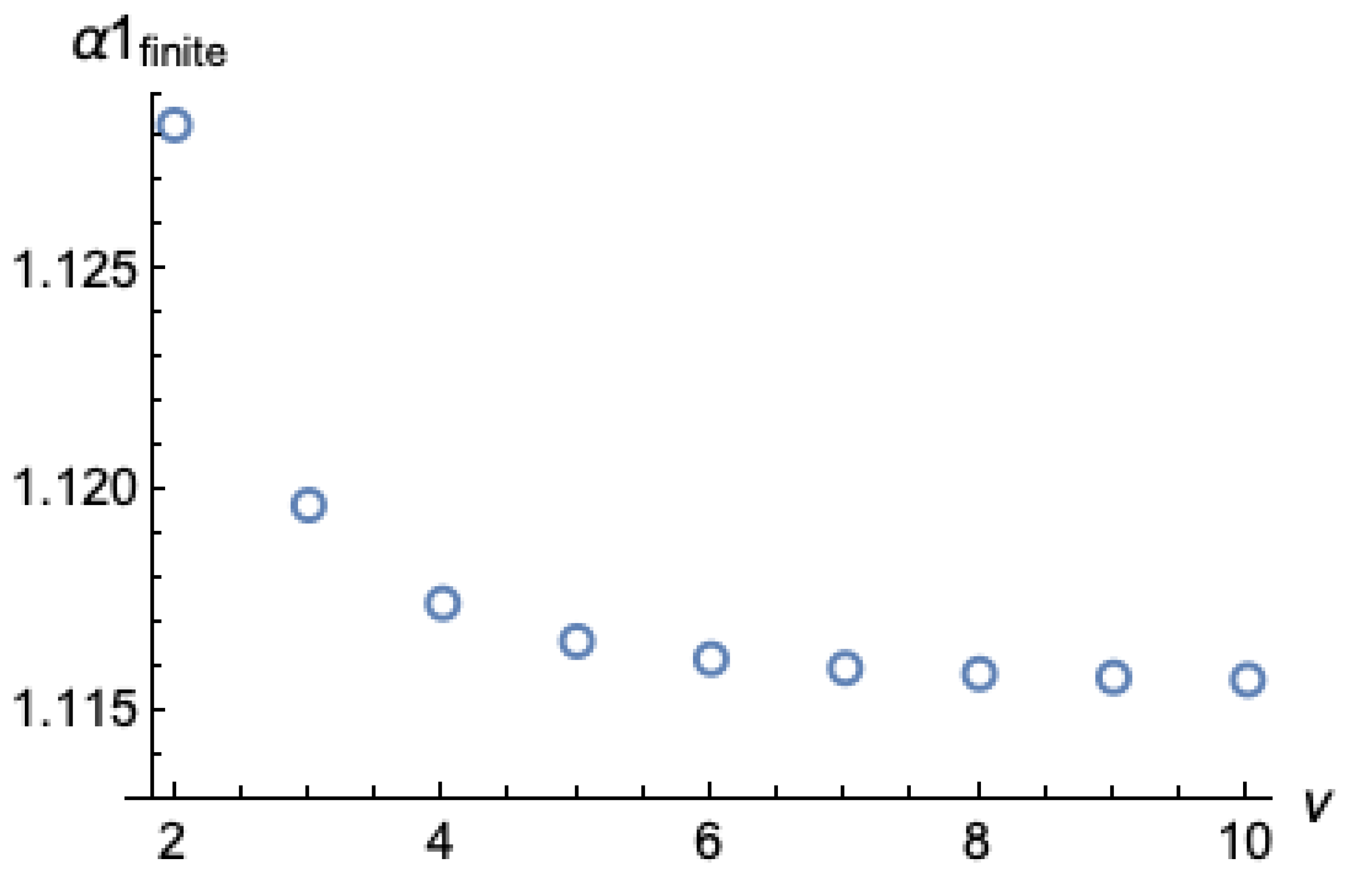
where any time dependence has been removed. The gradual approach of a 1 f to its exact value given by Equation (36) as the order ν of model (49) increases is shown in Figure 3.

3.1. Analysis and Application of the New Model

Seeking the best combination between accuracy and the lack of complexity, we present a full analysis by approximating expansion (44) to the 6th-order of x. In fact, the same analysis can be undertaken using an approximation of the 8th-order (the upper end of the meaningful model’s choices, in our opinion) in a similar manner, but the difficulty that is added while improving accuracy obscures the clarity of the presentation.
Specifically, by setting ν = 3, in Equation (44), we selected a 6th in terms of x, and expansion of the profile shape of the form
s x , t = 1 a 1 x 2 + a 2 x 4 + ( a 1 1 a 2 )   x 6
Correspondingly, Equation (48) for the evolution of a 1 ( t ) becomes
a 1   S o a 1 , a 2 S o , α 1 a ˙ 1 + S o , α 2 a ˙ 2 h o =   3 2   a 1 + a 2
In Equation (53), the storage S o a 1 , a 2 must be calculated numerically through the integral
S o ( t ) = 0 1 1 a 1   x 2 + a 2   x 4 + ( a 1 1 a 2 )     x 6   d x
while the partial derivatives S o , α 1 and S o , α 2 are calculated respectively through
S o , α 1 = S o a 1 = 1 2 0 1 x 2 + x 6 1 a 1   x 2 + a 2   x 4 + ( a 1 1 a 2 )   x 6   d x
and
S o , α 2 = S o a 2 = 1 2 0 1 x 4 x 6 1 a 1   x 2 + a 2   x 4 + ( a 1 1 a 2 )   x 6   d x
Equation (53) forms a close system in the context that was presented, together with Equation (48) for h o 1 ˙ = a 1 , and (27) for a 2 = a 1   2 h o 1   a ˙ 1 / 12 .
Before proceeding with the numerical solution of the defined system of equations, it is informative to have a closer look at the late-time behavior of this model. As the time derivatives vanish, the specific system of equations drives a 1 to a finite value (Figure 3), which can be found by solving Equation (49). With the present setting ν = 3, this corresponds to solving
a 1 S o = 3 2 a 1 + a 1 2 12
resulting in a 1 f = 1.11966 . Then, a 2 f = 1.11966 2 12 = 0.10447, and the finite shape function s(x) corresponds to a finite storage factor that is calculated (numerically) through (54), equal to S o f = 0.77269 . Thus, the slope of the squared shape function (42) becomes a 1 f   S o f = 0.86515 . These results are close but not identical to the exact asymptotic values given in Equations (35), (36), and (41) from the exact solution of the Boussinesq equation.
It is possible to refine the above values by slightly modifying the exact Equation (27), introducing a parameter c 1 as
12   a 2 = c 1 a 1   2 h o 1   a ˙ 1
This modification drives a 2 to a finite value of
a 2 f = c 1 a 1 f   2 12
Although affecting the exact character of Equation (27), one should keep in mind that the whole procedure that was described is an approximate solution, which is made as accurate as possible. Using (58) instead of (27) has the advantage of tuning the finite behavior of the solution toward more accurate values. Furthermore, this modification does not seriously affect the observed accuracy of the model at early times, where other types of problems should be handled, as will be shown.
By using c 1 as a tuning parameter, one may select the option resulting in the most accurate finite state through Equation (57), which now reads
a 1 f S o = 3 2 a 1 f + c 1 a 1 f   2 12
More specifically, we sought the value of c 1 , producing as accurately as possible the finite values for a 1 f and S o f as well as the slope of the squared profile. It was concluded that the best choice was c 1 = 0.9 . Using this value allowed for the calculations of a 1 f = 1.1156 ,   S o f = 0.7731 , and the slope of the squared shape a 1 f S o f = 0.8622 , showing agreement up to the 4th decimal when compared to the respective exact results of the Boussinesq equation.
At this point, it must be noted that in the case of an 8th-order expansion model (ν = 4), the added degree of freedom will guarantee the exact match of all three previous profile features, a 1 f , S o f , and correspondingly a 1 f S o f , by properly modifying the extra Equation (28) for   a 3 to close the model, with the inclusion of another tuning parameter c 2 through
360   a 3 = 2 c 2 a 1 3 5 a 1 a ˙ 1 ( t )   h o 1 + 12 a ˙ 2   h o 1 ( t )
In this case, the finite value of   a 3 f is a 3 f = c 2 a 1 3 180 , and the finite value for a 1 f comes from solving the analog of Equation (60) for the next higher order,
a 1 f S o = 4 3 a 1 f + 2 c 1 a 1 f 2 12 + c 2 a 1 f 3 180
finding the pair of ( c 1 , c 2 ) corresponding to the exact Boussinesq values for a 1 f and S o f .
Figure 4 presents the finite profile shape of the introduced 6th-order model
s ( x ) = 1 1.1156   x 2 + 0.1037 x 4 + 0.019 x 6
and the late-time exact Boussinesq solution by Equation (35). The coincidence between the two profiles was remarkable. In fact, their difference, at its most, did not exceed 1‰. Additionally, Figure 5, Figure 6 and Figure 7 provide the numerical solution of the full system of the model’s Equations (48), (53), and (58) for the evolution of the profile during drainage, where three different initializations were used to test the model’s efficiency.
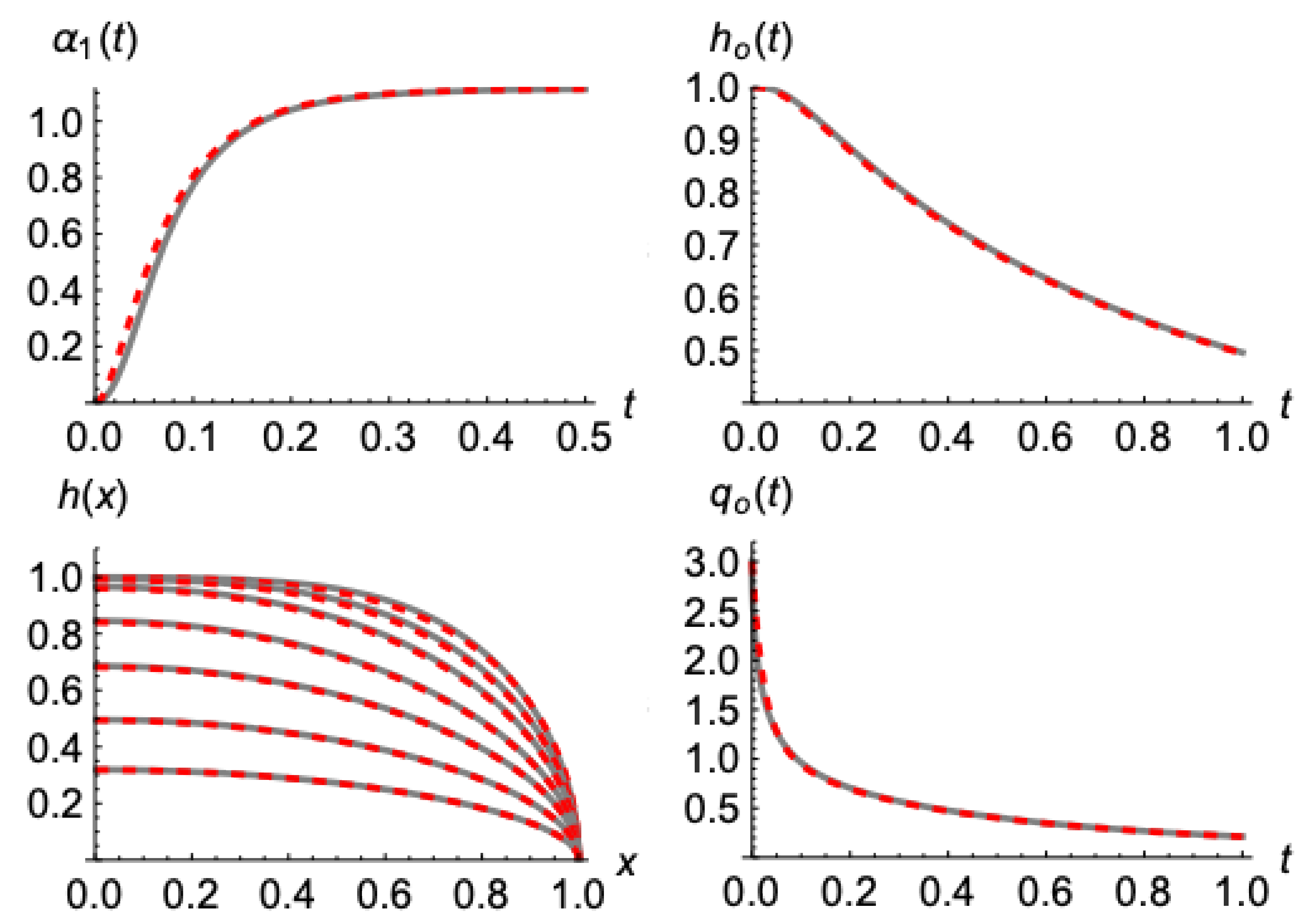
Specifically, in Figure 5, the case starts with the steady state after uniform recharging; thus, the initial profile is h x , 0 = 1 x 2 . The presented results refer to the evolutions of parameter a 1 t , the water table head, h o t = h ( 0 , t ) , water table h x , t , and outflow q o t . As shown, the resemblance of the model’s solution to the exact numerical solution of the Boussinesq Equation (11) is quite impressive. Even regarding the outflow, the most difficult parameter to capture accurately, since it is affected by the whole water profile’s development, the coincidence was very good. Aside from a relative difference at very early times that will be discussed next, the model performed very accurately.
Figure 6 and Figure 7 present similar results for the initial water tables of the forms h x , 0 = 1 x 4 and h x , 0 = 1 x 6 , respectively. The comparison remained adequately good and in favor of the presented model (49).
Taking a closer look, however, at the behavior of the outflow at very early times (Figure 8), one realizes that there is some discrepancy that increases as the initial outflow (thus the slope of the shape of the squared profile) becomes bigger.
This deviation can be attributed to the fact that the presented sharp initial water tables aimed to emulate the end of a recharging period and impose different physical characteristics compared to drainage profiles since they are not a solution of the same equation. Specifically, Boussinesq Equation (11) during pure drainage, with a zero-water depth (constant in the more general case) at the end of the aquifer, at x = 1, implies that the second derivative of the squared water profile versus x vanishes. This was not the case during recharge periods in any of the previously presented examples. To then conform with the imposed initial profile, Boussinesq concludes with a “violent” modification, resulting in a sudden change in outflow at an infinite rate, as will be shown. Multiplying Boussinesq Equation (11) during drainage by h(x,t) and differentiating versus x yields
  x   1 2 h ˙ x , t = x h x , t   1 2 2 h 2 ( x , t ) x 2 + h x , t   1 2 3 h 2 ( x , t ) x 3
Taking the limit of Equation (64) at x = 1 and substituting   q o t by Equation (19) shows that the time derivative of the outflow q ˙ o ( t ) equals
q ˙ o t = h x , t x x = 1   1 2 2 h 2 ( x , t ) x 2 x = 1
From Equation (65), kit becomes evident that, since the slope of the water profile at x = 1 is infinite, in order for q ˙ o t to be definite, the second derivative of the squared profile must be zero. Otherwise q ˙ o t is also infinite. Such behavior is, strictly speaking, beyond the capabilities of the presented model and demands different approximations to evolve up to a point that the model can accurately handle. Such a case is presented in Figure 9 for an initial squared profile with zero second derivative at x = 1, slightly different than the one presented in Figure 5. In this case, the coincidence between the present model and the Boussinesq solution was almost perfect.
Modeling the very early time drainage and matching it with the present model later on is the subject of the following section.

3.2. The Case of a Sudden Drawdown from an Initially Horizontal Water Table

This is a case that has been well-studied in the literature [7,26,27,28,29,30,31,32,33], resembling at the early stages a semi-infinite aquifer [26,27]. In a sense, it is an extreme example for applying modeling ideas starting with an infinitely sharp step-change. Still, it offers a great basis for analytic description and approximate solutions [26,31,33]. Our presented approximated solution cannot directly handle such extreme profiles accurately, as discussed earlier. However, intermediate modeling ideas can be used to confront such rough changes until the profile reaches a smoother shape that can be fed to the newly proposed model.

3.2.1. Early Time Approximation

The early behavior of the drainage can be approximated through a “wave type” character, in a way that is relatively similar to what [26] presented for the recharging built-up phase, of the form
h x , t = 1 ,       x < 1 Δ                                                                     Φ x 1 + Δ Δ ,         1 Δ < x < 1
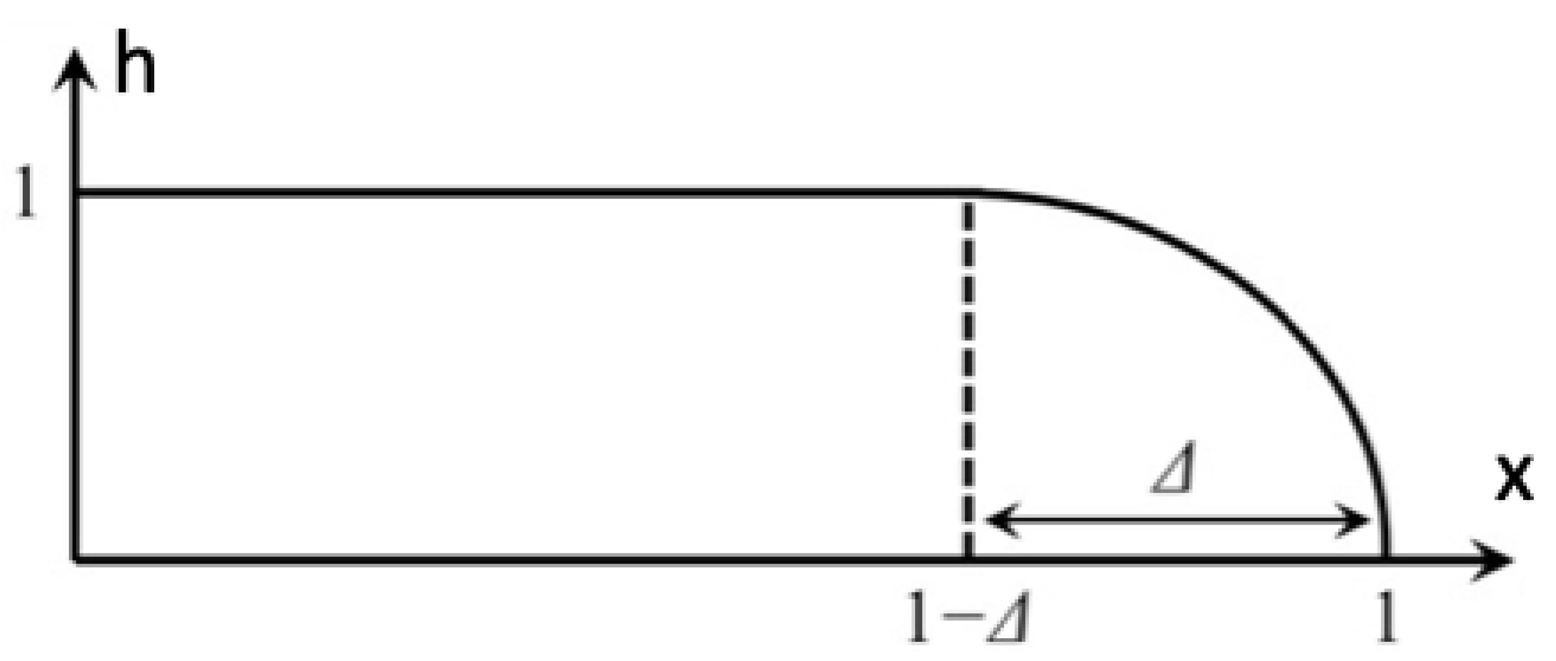
This means that the profile is uniform at the beginning and deforms gradually from the end point, x = 1, toward x = 0. The outflow affects the profile at a range Δ, starting from zero and increasing with time while keeping a constant shape Φ y in terms of y = x 1 Δ Δ , in a sense resembling a wave, as shown in Figure 10.
The dimensionless storage S t can be calculated by integrating the profile given in (66) through
S t = 0 1 h x , t   d x = 1 Δ t + Δ ( t ) 0 1 Φ y   d y
and by differentiation versus time, the outflow rate q t = S ˙ t reads
q ( t ) = S ˙ t = Δ ˙ t 1 0 1 Φ y   d y
Recalling the detailed analysis given in [7,27], the actual outflow for this specific case of a sudden drawdown and drainage shows a behavior of the form
q t = s 1   t 1 / 2
with s 1 0.33206 [7]. In order to reproduce this behavior by the modeled Equation (68), the velocity of the wave, Δ ˙ t , must show a time dependence of the form
Δ ˙ t = s 1   1 0 1 Φ y   d y 1 t 1 / 2
which obviously becomes infinite at the beginning of the drainage, in agreement with the initially infinite outflow rate at this specific case. Integrating Equation (70) over time then results in the model’s gradual displacement
Δ t = 2 s 1   1 0 1 Φ y   d y 1 t 1 / 2
What remains is to specify a proper form for Φ y . Along the same line as the analysis followed in the previous section, it was assumed that Φ y can be described by a polynomial of the form
Φ y = 1 + a 2   y 4 + a 3   y 6 + a ν y 2 ν
with a ν = 1 a 2   a 3   a ν 1   . The specific form satisfies the proper boundary conditions Φ 0 = 1 and Φ 1 = 0 , and the absence of the y 2 term guarantees the vanishing of the three first derivatives at y = 0, providing a smooth transition between the two branches of the model (66). Furthermore, after the end of the functionality of the model (66), at the time when Δ t = 1 and the “wave” reaches the upper end at x = 0, the evolution of the water profile can be continued using the analysis presented in the previous section.
Making use of the mass-balance integrated Boussinesq equation, the outflow should match the dimensionless slope of the squared profile at x = 1 through
q ( t ) = 1 2 lim x 1 h 2 ( x , t ) x = 1 2 Δ ( t ) Φ 2 ( y ) y y = 1
After calculating the dimensionless slope of the modeled Φ 2 y at y = 1
Φ 2 1 2 = ν + ν 2 a 2 + ν 3 a 3 + 2 a ν 2 + a ν 1
and introducing it into Equation (73), the mass balance yields
2 1 0 1 Φ y   d y 1 = ν + ν 2 a 2 + 2 a ν 2 + a ν 1 s 1   2
which offers a closure of the “wave” model (66), linking the dimensionless storage 0 1 Φ y   d y with the parameters of the model, a 2 ,   a 3 and so on. In fact, Equation (75) offers many degrees of freedom, thus, giving the opportunity to investigate and impose several specific features in the assumed “wave shape”. However, for the sake of simplicity and in the context of the previous section, we present the simplest and most meaningful model with ν = 3, which is expressed as
Φ y = 1 + a 2   y 4 + ( 1 a 2   ) y 6
Through this choice, Equation (75) is reduced to
1 0 1 1 + a 2   y 4 ( 1 + a 2   )   y 6   d y 1 = 3 + a 2 2 s 1   2
allowing for the direct numerical estimation of the proper value of a 2 = 1.4818945 . With this value of a 2 , the dimensionnless storage equals, S o = 0 1 Φ y   d y = 0.854735 . The model is valid up to the limiting time, tmax, when the “wave” reaches the upper end at x = 0, which is calculated through Equation (71) and equals tmax = 0.0478442, for Δ t = 1 .
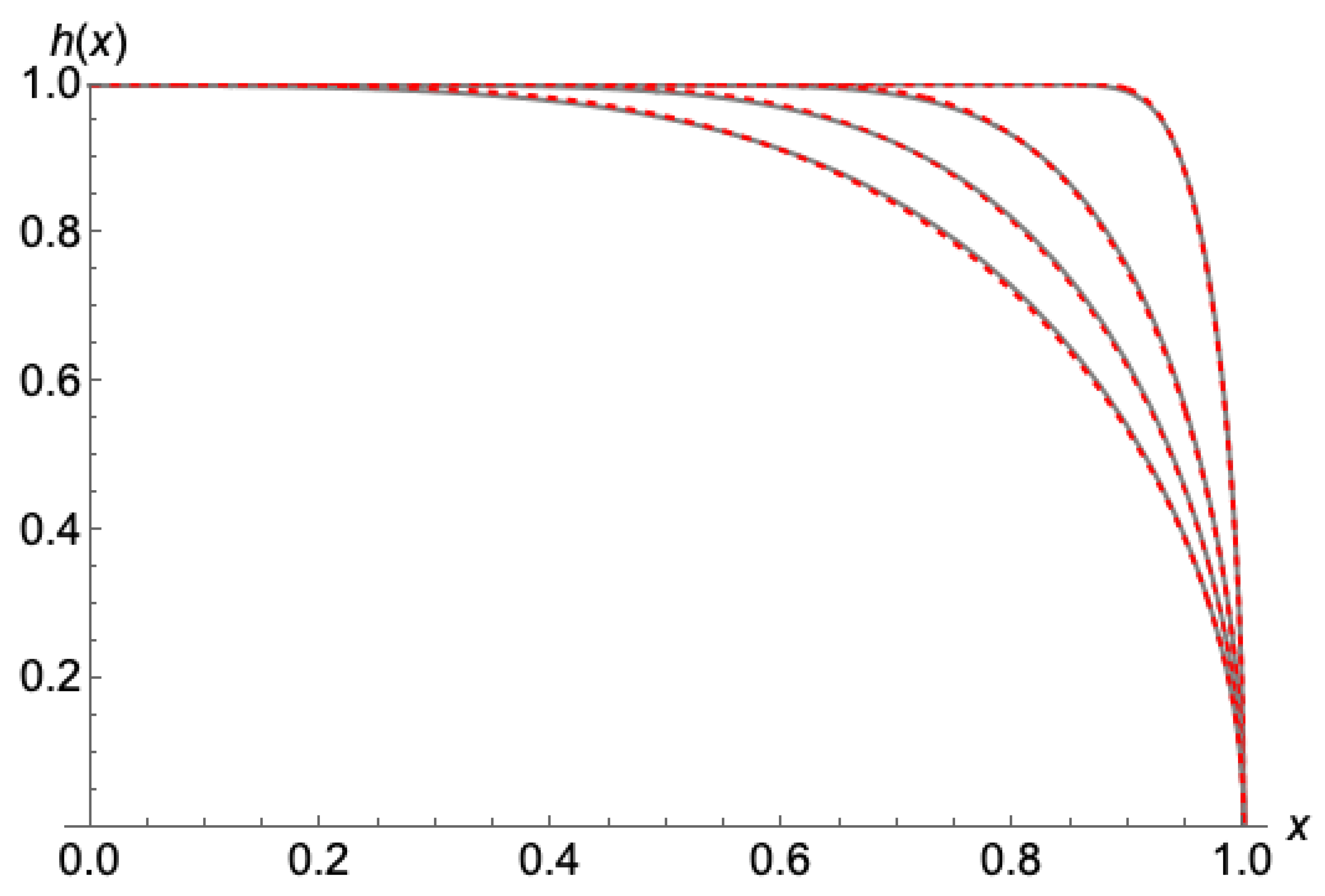
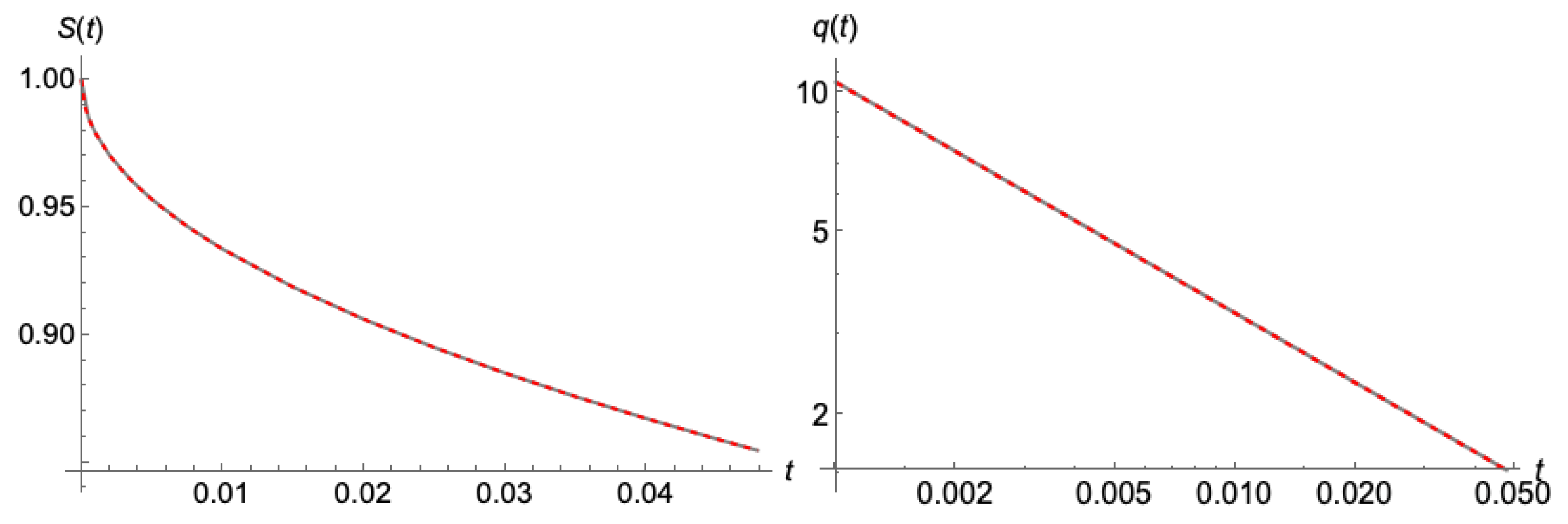
Applying the above, we present the evolution of the water depth (Figure 11) and the water storage and outflow (Figure 12) from the present “wave” model and the exact numerical solution of Boussinesq (3), starting from a horizontal initial profile and continuing up to time t = 0.0478442. The coincidence between the “wave” approximation (66) and Boussinesq Equation (3) was remarkable regarding the profile evolution (Figure 10), and became exact in the case of the mass balance and the outflow (Figure 12).

3.2.2. Later Times

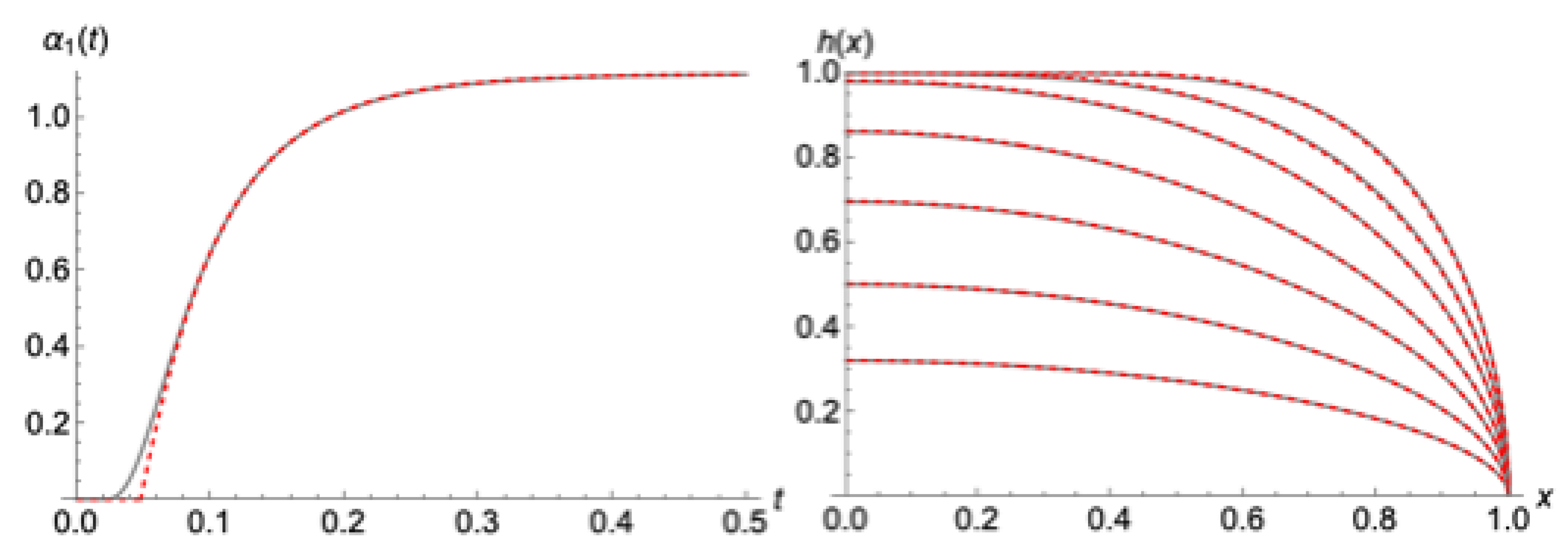
At the limiting time tmax = 0.0478442, when the wave reached the upper end at x = 0, we made use of the new model (54) starting with the profile s x = Φ ( x ) from Equation (76) and continued by numerically solving the system of equations as analyzed in Section 3.1. As shown in Figure 13, even though parameter a 1 t started from a zero value in the modeled solution while the exact Boussinesq proceeded (meaning that the head of the water table had already started decreasing slightly from 1, at tmax), both solutions very quickly matched. This matching also correctly drove the general pattern of the water table evolution, which was impressively captured.
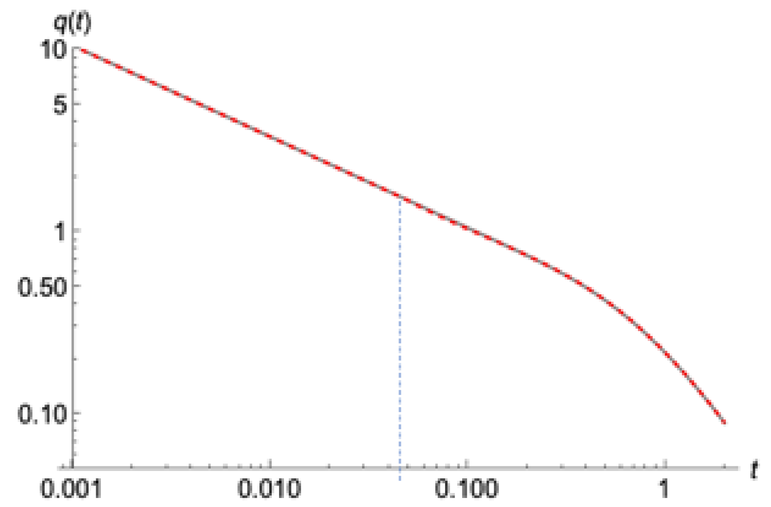
The outflow q o t also showed a nice passage from the “wave” period of the solution to the new model (53), which almost perfectly matched the exact Boussinesq (Figure 14). Unlike the cases presented in Section 3.1, the Boussinesq has now entered a more “mature” state, satisfying the condition (65), thus the behavior of q ˙ t is much smoother at the increment of time t = tmax. Such behavior is exactly what the new model can capture very accurately.
The above analysis, together with the findings of the previous section regarding the initial “irregularity” when recharging stops and pure drainage begins, paves the way for exploring the very early time of departing from any recharging period to drainage. Intuitively, one can guess departures of the form q o t = q o 0 k   t z , 0 < z < 1 into the behavior of the outflow, but this is a matter for future research.

3.3. An Analytic Explicit Linear Approximation for the Solution of the New Model

In this last section, we present the approximation of the nonlinear system of Equations (48), (53) and (58) of the previously introduced and analyzed model with a linear form, allowing for an analytical explicit solution for a 1 ( t ) and the rest of the parameters, which was proven to be accurate and well-understood.
Substituting into the mass balance the main Equation (53) a 1   S o + h o 1   S o , α 1 a ˙ 1 + S o , α 2 a ˙ 2 =   3 2   a 1 + a 2 of the model that was presented,   a 2 = 0.9   a 1   2 h o 1   a ˙ 1 /12 by Equation (58), and its first derivative a ˙ 2 by
  a ˙ 2 = 0.8 a 1 a ˙ 1 h o 1   a ¨ 1 12
one concludes with
a 1   S o + 2 0.9   a 1 12 + a ˙ 1 h o 1 1   12 S o , α 1 S o , α 2 0.8 a 1 12 +   a ¨ 1 h o 2 S o , α 2 12 = 3
Then, dividing (79) with the multiplier of the term a 1 , S o + 2 0.9   a 1 12 , the mass balance equation equivalently reads
a 1 + a ˙ 1 h o 1 1   12 S o , α 1 S o , α 2 0.8 a 1 12 S o + 2 0.9   a 1 12 +   a ¨ 1 h o 2 S o , α 2 12 S o + 2 0.9   a 1 12 = 3 S o + 2 0.9   a 1 12
which is obviously a second-order nonlinear differential equation of a 1 ( t ) of the form
A ( a 1 )   a ¨ 1 + B ( a 1 )   a ˙ 1 + a 1 = C ( a 1 )
When the time derivatives vanish, Equations (79)–(81) yield
a 1 = C a 1   = 3 S o ( a 1 ) + 2 0.9   a 1 12
which is exactly the late-time solution by Equation (60), defining the finite value of parameter a 1 , a 1 f . Noting that in Equation (81) the function C a 1 does not vary strongly (i.e., the denominator typically varies in a range between 2.6 and 2.9 for most cases), C a 1 in Equation (81) can be nicely approximated by its finite value C a 1 = a 1 f ,
A ( a 1 )   a ¨ 1 + B ( a 1 )   a ˙ 1 + a 1 = a 1 f
assuring that a 1 reaches the correct finite state a 1 f . Then, in a rather crude way, Equation (83) can be simplified further to the linear form
A a ¨ 1 + B   a ˙ 1 + a 1 = a 1 f
where the time dependent nonlinear terms A ( a 1 ) and B a 1 are approximated with the constants A, B. Equation (84) is the linear approximation of the exact Equation (80).
We saw, quite intuitively, that the best choice for the linearization constant values came through demanding Equation (84) satisfy the exact initial values of a 1 ( 0 ) , a 10 , and its derivatives at time zero, a 10 ,   a ¨ 10 ,   a ˙ 10 , as they were defined by the exact setup. In this way, Equation (84) correctly incorporates the initial and finite behavior of the original nonlinear system. Specifically, by demanding A and B to satisfy the system
A a ¨ 10 + B   a ˙ 10 + a 10 = a 1 f A a 10 + B   a ¨ 10 + a ˙ 10 = 0
and by solving, one concludes with the desirable values
A =   a 1 f a ¨ 10 a 10 a ¨ 10 + a ˙ 10 a ˙ 10 a ¨ 10 2 a 10 a ˙ 10 ,   B = a ˙ 10 A a 10 a ¨ 10
Noting that A and B are positive and that they differ by two-orders of magnitude, the solution of (84) is always meaningful and can be expressed straight-forward into the form
a 1 t = a 1 f 1 d 1   e w 1 t d 2 e w 2 t
with w 1 and w 2 to be given by
  w 1 = B + B 2 4 A 2 A ,     w 2 = B B 2 4 A 2 A
and d 1 , d 2 by
  d 1 = B + B 2 4 A 2 A ,   d 2 = 1 d 1 + a 10 a 1 f
After that, the integration of Equation (87) over time gives, through Equation (23), the evolution of the water table head at x = 0, h o t , in the form
h o 1 t = 1 + a 1 f   t + a 1 f   d 1 w 1   e w 1 t 1 + a 1 f   d 2 w 2 e w 2 t 1
The remaining parameter   a 2 is also calculated by Equation (58) as   a 2 = 0.9   a 1   2 h o 1   a ˙ 1 /12. With these parameters, the analytic approximation for the solution of the model is now completed, and the work may procced with the testing of its performance.
In Figure 15, we present the comparison between the evolutions of a 1 t , a 2 t , and outflow q o t = h o 2 t 3 2   a 1 ( t ) +   a 2 ( t ) as they are calculated numerically from the exact presented model in Section 3.1, and analytically by its explicit linear approximation (89)–(90). All previous initializations that have been discussed so far were used, corresponding to an initial s x , 0 equal to 1 x 2 , 1 x 4 , 1 x 6 , and 1 1.5 x 4 + 0.5 x 6 . We also added a more “exotic”, non-monotonous initial profile equal to 1 + 0.5 x 2 + 1.5 x 4 3 x 6 . As shown, the performance of the analytical expression (89) in estimating a 1 t was overall very good, with an accuracy to the order of 5‰ at its worst. This also led to the accurate calculation of the remaining parameters, especially the outflow, the most difficult one, with an accuracy to the order of ±1% in the worst case. In this way, expressions (89) and (90) may serve as easy and accurate representation for both the investigation and understanding of the drainage flow as well as a modeling basis for handling more real cases.
In conclusion, it should be noted that the same linearization idea can be applied in the case of a more accurate and detailed model of the 8th-order by calculating three linearization parameters, in this case
A a 1 + B   a ¨ 1 + C a ˙ 1 + a 1 = a 1 f
which yields a solution for a 1 t of the form
a 1 t = a 1 f 1 d 1   e w 1 t d 2 e w 2 t d 3 e w 3 t
However, finding the proper linearization values for constants A, B, and C is much more complicated and requires special attention to satisfy much stricter criteria for the solution to be well-behaved.

4. Conclusions

In this work, conceptual approximations of the Boussinesq equation for horizontal unconfined aquifers during the pure drainage phase, without any recharge and zero-inflow conditions, were introduced and analyzed. A variety of methods were utilized, which included wave solution, variable separation, and series expansion, to construct a new model and explore its behavior and performance against the Boussinesq equation and its exact (non-closed form) solution at early and later times. The new model is based on the relations between the parameters defining the water table shape as they are implied by the Boussinesq equation. To close the system of equations, the mass conservation principle was employed. The model proved to perform quite accurately for several initial water tables, becoming almost exact at the later times.
At the very early times, there were some affordable deviations from the exact Boussinesq, which were physically attributed to the different natures of the recharging phase compared to the pure drainage period. As was proven, in order to conform the imposed initial profile after recharge, Boussinesq concludes with a “violent” modification, resulting in a sudden change in outflow at an infinite rate. Modeling ideas in the form of a “wave” were discussed and applied to describe such rough changes until the profile reached a smoother shape that could be fed to the newly proposed model, resulting in the best accuracy.
The modeled nonlinear forms were finally linearized, concluding with explicit analytical expressions incorporating most of the basic characteristics regarding the evolution of the water table and the outflow from the exact Boussinesq equation under different initial conditions.
The results from this research can be used as benchmarks for numerical modeling and serve as the basis for further theoretical development in groundwater hydrology with practical importance. Plausibly, these ideas could be further exploited to build simple but effective models for the very early behavior of drainage flow after any initial water table is formed during the recharging period. Furthermore, they can be extended to also describe the built-up phase during recharge, resulting into a complete tool. This will be the subject of future work by the authors.

Author Contributions

Conceptualization, E.A. and E.G.; Methodology, E.A. and E.G.; Software, E.A. and E.G.; Formal analysis, E.A. and E.G.; Writing—original draft, E.A. and E.G.; Writing—review & editing, E.A. and E.G. All authors have read and agreed to the published version of the manuscript.

Funding

This research received no external funding.

Data Availability Statement

Data is contained within the article.

Conflicts of Interest

The authors declare no conflict of interest.

References

  1. Boussinesq, J. Essai sur la theorie des eaux courantes du mouvement nonpermanent des eaux souterraines. Acad. Sci. Inst. Fr. 1877, 23, 252–260. [Google Scholar]
  2. Boussinesq, J. Recherches theoriques sur l’ecoulement des nappes d’eau infiltrees dans le sol et sur debit de sources. J. Math. Pures Appl. 1904, 10, 5–78. [Google Scholar]
  3. Dupuit, J. Etudes Theoriques et Practiques sur le Mouvement des Eaux dans les Canaux Decouverts et a Travers les Terrains Permeables, 2nd ed.; Dunod: Paris, France, 1863. [Google Scholar]
  4. Forchheimer, P. Über die Ergiebigkeit von Brunnen-Anlagen und Sickerschlitzen. Z. Architekt. Ing.-Ver. Hann. 1886, 32, 539–563. [Google Scholar]
  5. Wooding, R.A.; Chapman, T.G. Groundwater flow over a sloping impermeable layer: 1. Application of the Dupuit-Forchheimer assumption. J. Geophys. Res. 1966, 71, 2895–2902. [Google Scholar] [CrossRef]
  6. Barenblatt, G.I. On some unsteady fluid and gas motions in a porous medium. J. Appl. Math. Mech. 1952, 16, 67–78. [Google Scholar]
  7. Polubarinova-Kochina, P.Y. Theory of Ground Water Movement; Princeton University Press: Princeton, NJ, USA, 1962. [Google Scholar]
  8. Barenblatt, G.I.; Entov, V.M.; Ryzhik, V.M. Theory of Fluid Flows through Natural Rocks; Kluwer Academic Publishers: Dordrecht, The Netherlands, 1990. [Google Scholar]
  9. Chen, Z.X.; Bodvarsson, G.S.; Witherspoon, P.A.; Yortsos, Y.C. An integral equation formulation for the unconfined flow of groundwater with variable inlet conditions. Trans. Porous Media 1995, 18, 15–36. [Google Scholar] [CrossRef]
  10. Lockington, D.A.; Parlange, J.Y.; Parlange, M.B.; Selker, J. Similarity solution of the Boussinesq equation. Adv. Water Resour. 2000, 23, 725–729. [Google Scholar] [CrossRef]
  11. Parlange, J.Y.; Hogarth, W.L.; Govindaraju, R.S.; Parlange, M.B.; Lockington, D. On an exact analytical solution of the Boussinesq equation. Trans. Porous Media 2000, 39, 339–345. [Google Scholar] [CrossRef]
  12. Telyakovskiy, A.S.; Braga, G.A.; Furtado, F. Approximate similarity solutions to the Boussinesq equation. Adv. Water Resour. 2002, 25, 191–194. [Google Scholar] [CrossRef]
  13. Pistiner, A. Similarity solution to unconfined flow in an aquifer. Trans. Porous Media 2008, 71, 265–272. [Google Scholar] [CrossRef]
  14. Moutsopoulos, N. Solutions of the Boussinesq equation subject to a nonlinear Robin boundary condition. Water Resour. Res. 2013, 49, 7–18. [Google Scholar] [CrossRef]
  15. Basha, H.A. Traveling wave solution of the Boussinesq equation for groundwater flow in horizontal aquifers. Water Resour. Res. 2013, 49, 1668–1679. [Google Scholar] [CrossRef]
  16. Basha, H.A. Perturbation solutions of the Boussinesq equation for horizontal flow in finite and semi-infinite aquifers. Adv. Water Resour. 2021, 155, 104016. [Google Scholar] [CrossRef]
  17. Chor, T.; Ruiz de Zarate, A.; Dias, N.L. A generalized series solution for the Boussinesq equation with constant boundary conditions. Water Resour. Res. 2019, 55, 3567–3575. [Google Scholar] [CrossRef]
  18. Chor, T.; Dias, N.L.; Ruiz de Zárate, A. An exact series and improved numerical and approximate solutions for the Boussinesq equation. Water Resour. Res. 2013, 49, 7380–7387. [Google Scholar] [CrossRef]
  19. Tzimopoulos, C.; Papadopoulos, K.; Papadopoulos, B.; Samarinas, N.; Evangelides, C. Fuzzy solution of nonlinear Boussinesq equation. J. Hydroinformatics 2022, 24, 1127–1147. [Google Scholar] [CrossRef]
  20. Hayek, M. A simple and accurate closed-form analytical solution to the Boussinesq equation for horizontal flow. Adv. Water Resour. 2024, 185, 104628. [Google Scholar] [CrossRef]
  21. Tzimopoulos, C.; Samarinas, N.; Papadopoulos, K.; Evangelides, C. Fuzzy Analytical Solution for the Case of a semi-Infinite Unconfined Aquifer. Environ. Sci. Proc. 2023, 25, 70. [Google Scholar] [CrossRef]
  22. Ceretani, A.; Falcini, F.; Garra, R. Exact solutions for the fractional nonlinear Boussinesq equation. In Proceedings of the INdAM Workshop on Fractional Differential Equations: Modeling, Discretization, and Numerical Solvers, Singapore, 8 March 2023; Springer Nature: Singapore, 2023. [Google Scholar]
  23. Animasaun, I.L.; Shah, N.A.; Wakif, A.; Mahanthesh, B.; Sivaraj, R.; Koriko, O.K. Ratio of Momentum Diffusivity to Thermal Diffusivity: Introduction, Meta-analysis, and Scrutinization; Chapman and Hall/CRC: New York, NY, USA, 2022; ISBN 13: 978-1032108520/10: 1032108525/9781003217374. [Google Scholar] [CrossRef]
  24. Akylas, E.; Gravanis, E.; Koussis, A.D. Quasi-steady flow in sloping aquifers. Water Resour. Res. 2015, 51, 9165–9181. [Google Scholar] [CrossRef]
  25. Gravanis, E.; Akylas, E.; Sarris, E. Approximate Solutions for Horizontal Unconfined Aquifers in the Buildup Phase. Water 2024, 16, 1031. [Google Scholar] [CrossRef]
  26. Gravanis, E.; Akylas, E. Early-time solution of the horizontal unconfined aquifer in the buildup phase. Water Resour. Res. 2017, 53, 8310–8326. [Google Scholar] [CrossRef]
  27. Lockington, D.A. Response of unconfined aquifer to sudden change in boundary head. J. Irrig. Drain. Eng. 1997, 123, 24–27. [Google Scholar] [CrossRef]
  28. Parlange, J.Y.; Stagnitti, F.; Heilig, A.; Szilagyi, J.; Parlange, M.B.; Steenhuis, T.S.; Hogarth, W.L.; Barry, D.A.; Li, L. Sudden drawdown and drainage of a horizontal aquifer. Water Resour. Res. 2001, 37, 2097–2101. [Google Scholar] [CrossRef]
  29. Akylas, E.; Koussis, A.D. Response of sloping unconfined aquifer to stage changes in adjacent stream I. Theoretical analysis and derivation of system response functions. J. Hydrol. 2007, 338, 85–95. [Google Scholar] [CrossRef]
  30. Koussis, A.D.; Akylas, E.; Mazi, K. Response of sloping unconfined aquifer to stage changes in adjacent stream II. Applications. J. Hydrol. 2007, 338, 73–84. [Google Scholar] [CrossRef]
  31. Koussis, A.D.; Akylas, E. Slug Test in Confined Aquifers, the Over-Damped Case: Quasi-Steady Flow Analysis. Groundwater 2012, 50, 608–613. [Google Scholar] [CrossRef]
  32. Moutsopoulos, K.N. The analytical solution of the Boussinesq equation for flow induced by a step change of the water table elevation revisited. Trans. Porous Med. 2010, 85, 919–940. [Google Scholar] [CrossRef]
  33. Jiang, Q.; Tang, Y. A general approximate method for the groundwater response problem caused by water level variation. J. Hydrol. 2015, 529, 398–409. [Google Scholar] [CrossRef]
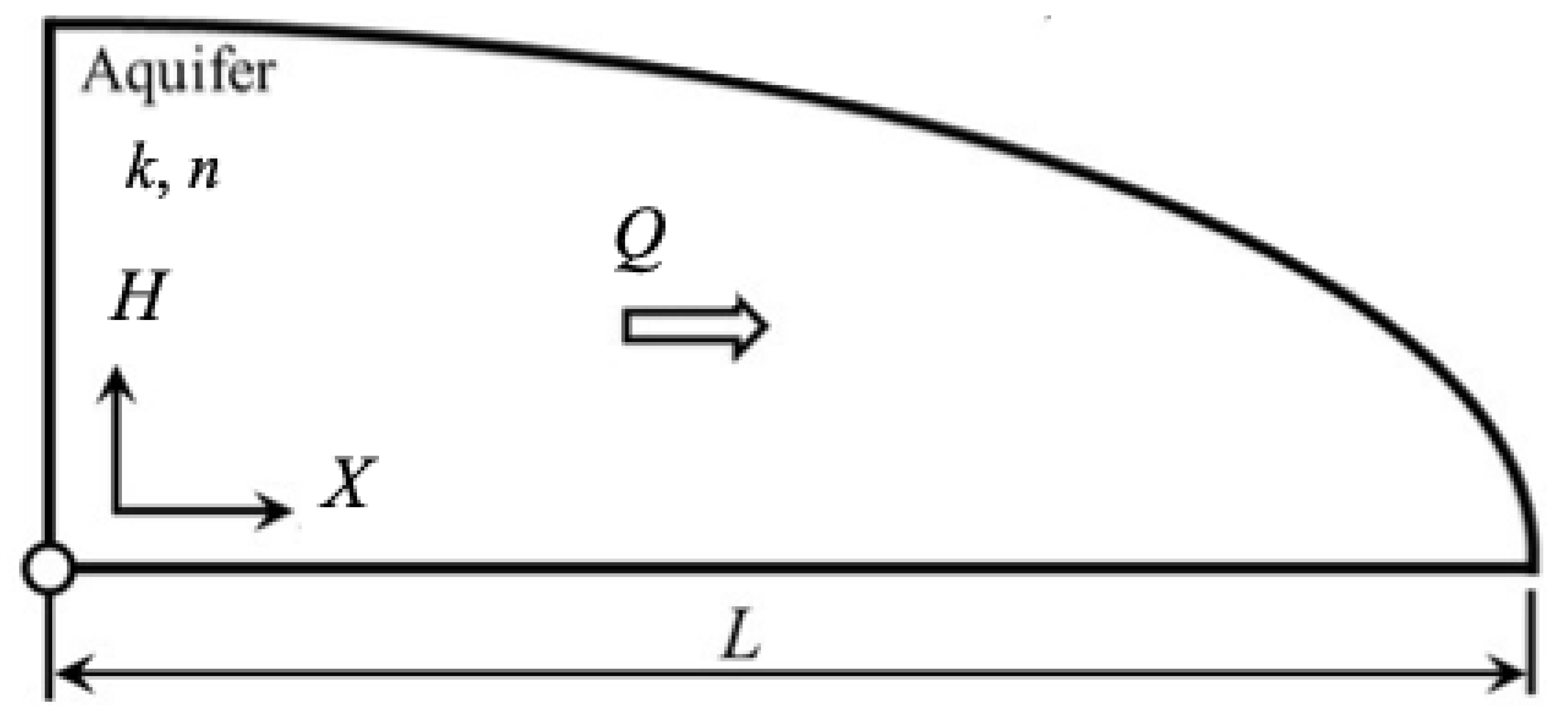
Figure 1. Cross-sectional schematic diagram of a horizontal soil layer with constant and uniform hydraulic conditions during the pure drainage period.
Water 16 02984 g001
Figure 2. Cross-sectional schematic diagram of a horizontal soil layer with constant and uniform hydraulic conditions during the pure drainage period with two well-separated initial conditions. The steady state (9) after constant recharge of an infinite period (continuous line) and a uniform horizontal water table (10) (dashed line).
Water 16 02984 g002
Figure 3. The gradual approach of a 1 f to its exact value given by Equation (36) as the order ν of model (49) increases.
Water 16 02984 g003
Figure 4. The perfect coincidence between the finite late-time state calculated by the new model (red dashed line) through Equation (63) and the exact solution of the Boussinesq (gray line) Equation (34).
Water 16 02984 g004
Figure 5. The excellent coincidence between the present model’s (Equation (53)) numerical application (red dashed lines) and the numerical solution of the exact Boussinesq equation (gray lines) for the drainage phase after an initial h x , 0 = 1 x 2 profile. The evolution histories for (from the upper left corner and continuing clockwise) the parameter a 1 t , the water table head h o t = h ( 0 , t ) , the outflow q o t , and the water table h x , t (at times 0.025, 0.05, 0.1, 0.25, 0.5, 1, 2).
Water 16 02984 g005
Figure 6. As in Figure 5, for h x , 0 = 1 x 4 initially.
Water 16 02984 g006
Figure 7. As in Figure 5, for h x , 0 = 1 x 6 initially.
Water 16 02984 g007
Figure 8. Evolution of outflow q o t at very early times from the present model’s (Equation (54)) numerical application (red dashed lines) and the numerical solution of the exact Boussinesq equation (gray lines) for the drainage phase after the initial profiles h x , 0 = 1 x 2 , 1 x 4 and 1 x 6   (left to right).
Water 16 02984 g008
Figure 9. Evolution of outflow q o t at very early times from the present model’s (Equation (54)) numerical application (red dashed lines) and the numerical solution of the exact Boussinesq equation (gray lines) for drainage phase after initial profile h 2 x , 0 = 1 x 2 1 9 x 4 + 1 9 x 6 .
Water 16 02984 g009
Figure 10. Schematic representation of the water profile during the early drainage phase of the horizontal aquifer.
Water 16 02984 g010
Figure 11. The agreement during the evolution of the water depth h ( x , t ) at early times between the full numerical solution (gray lines) and the present “wave” model (red dashed lines) at times 0.001, 0.01, 0.025, 0.0478442 (time increased downward), starting from an initially horizontal profile.
Water 16 02984 g011
Figure 12. The exact agreement of the evolution of the water storage S t = 0 1 h ( x , t ) d x and the outflow q 0 t , at early times between the exact numerical solution of Boussinesq (gray lines) and the present “wave” model with S t = 1 2 s 1 t and q t = s 1   t 1 / 2 (red dashed lines), starting from an initially horizontal profile.
Water 16 02984 g012
Figure 13. The evolution histories of the parameter a 1 t   (left), and the water table h x , t (at times 0.025,0.05, 0.1, 0.25, 0.5, 1, 2) by the numerical solution of the exact Boussinesq Equation (3) (gray lines) and from the present wave approximation, which was continued by the new model’s (Equation (53)) numerical application (red dashed lines).
Water 16 02984 g013
Figure 14. Evolution of the outflow from the full numerical solution (gray lines) and the combination of the “wave” model at early times and the 6th-order model later on (red dashed lines). tmax is also shown (blue dushed line) for better interpretation.
Water 16 02984 g014
Figure 15. Comparison of the evolution of a 1 t , a 2 t , and outflow, q o t , (right to left) by the numerical solution of the presented model (gray lines) and its analytic linear approximation (red dashed lines). Different initializations (up to down) correspond to s x , 0 equal to: 1 x 2 , 1 x 4 , 1 x 6 , 1 1.5 x 4 + 0.5 x 6 , and 1 + 0.5 x 2 + 1.5 x 4 3 x 6 .
Water 16 02984 g015
Disclaimer/Publisher’s Note: The statements, opinions and data contained in all publications are solely those of the individual author(s) and contributor(s) and not of MDPI and/or the editor(s). MDPI and/or the editor(s) disclaim responsibility for any injury to people or property resulting from any ideas, methods, instructions or products referred to in the content.