Abstract
Water is a vital resource, and its quality has a direct impact on human health. Groundwater, as one of the primary water sources, requires careful monitoring to ensure its safety. Although manual methods for testing water quality are accurate, they are often time-consuming, costly, and inefficient when dealing with large and complex data sets. In recent years, machine learning has become an effective alternative for water quality assessment. However, current approaches still face challenges, such as the limited performance of individual models, minimal improvements from optimization algorithms, lack of dynamic feature weighting mechanisms, and potential information loss when simplifying model inputs. To address these challenges, this paper proposes a hybrid model, BS-MLP, which combines GBDT (gradient-boosted decision tree) and MLP (multilayer perceptron). The model leverages GBDT’s strength in feature selection and MLP’s capability to manage nonlinear relationships, enabling it to capture complex interactions between water quality parameters. We employ Bayesian optimization to fine-tune the model’s parameters and introduce a feature-weighting attention mechanism to develop the BS-FAMLP model, which dynamically adjusts feature weights, enhancing generalization and classification accuracy. In addition, a comprehensive parameter selection strategy is employed to maintain data integrity. These innovations significantly improve the model’s classification performance and efficiency in handling complex water quality environments and imbalanced datasets. This model was evaluated using a publicly available groundwater quality dataset consisting of 188,623 samples, each with 15 water quality parameters and corresponding labels. The BS-FAMLP model shows strong classification performance, with optimized hyperparameters and an adjusted feature-weighting attention mechanism. Specifically, it achieved an accuracy of 0.9616, precision of 0.9524, recall of 0.9655, F1 Score of 0.9589, and an AUC score of 0.9834 on the test set. Compared to single models, classification accuracy improved by approximately 10%, and when compared to other hybrid models with additional attention mechanisms, BS-FAMLP achieved an optimal balance between classification performance and computational efficiency. The core objective of this study is to utilize the acquired water quality parameter data for efficient classification and assessment of water samples, with the aim of streamlining traditional laboratory-based water quality analysis processes. By developing a reliable water quality classification model, this research provides robust technical support for water safety management.
1. Introduction
Water, as the medium for all chemical reactions within living organisms, plays an indispensable role in maintaining the ecological balance and ensuring life activities. [1]. In developing countries, 80% of illnesses are caused by unsafe drinking water and poor sanitation conditions, according to the World Health Organization [2]. Water is an important resource for agricultural irrigation, industrial production, and people’s lives. Its quality directly affects agriculture, economic development, and human health [3]. Therefore, accurately and effectively classifying water quality has become an important research hotspot in environmental science.
Traditionally, the classification and evaluation of water samples have relied on chemical analysis and physical measurements, such as laboratory tests for the concentrations of chemical components in water, followed by manual analysis based on expert experience to assess water quality using relevant standards [4]. Although these methods provide precise water quality data, they are often time-consuming, costly, and dependent on expensive equipment. Moreover, traditional approaches are limited by the small number of samples and insufficient spatial coverage, making large-scale water quality monitoring difficult, particularly in complex and dynamic groundwater systems, where these methods face increasing limitations [5].
Among emerging approaches, the adaptability to large data sets and high accuracy of machine learning have attracted the attention of researchers [6]. Machine learning can learn and understand water quality characteristics and trends by training on datasets, allowing for accurate water quality classification [7]. With this technology, not only can abnormal water quality samples be effectively detected, but model performance can also be evaluated using various parameters [8,9]. This method offers not only precise classification but also insights into the key drivers of water quality changes, thus providing valuable guidance for water quality management and evaluation [10,11].
Researchers have increasingly applied machine learning techniques to the classification and prediction of water quality in recent years. S. Mahdi Saghebian et al. (2013) proposed a decision tree (DT)-based method for groundwater quality classification in the Ardabil region of Iran. They combined the U.S. Salinity Laboratory (USSL) diagram with monthly precipitation data and water chemical parameters. Their findings showed that DT offered higher accuracy and efficiency compared to Principal Component Analysis (PCA), especially when handling nonlinear data [12].
Salisu Yusuf Muhammad et al. (2015) developed a classifying model for detecting and predicting water quality. This study explored various machine learning models, including DT, Support Vector Machines (SVMs), and Random Forests (RFs), ultimately selecting the five best-performing models for comparison and evaluation. The research showed that machine learning models exhibited good adaptability in water quality classification tasks, particularly when dealing with complex high-dimensional data [13].
H. H. Khamees et al. (2018) used an approach combining parametric (IPNOA) and multivariate data-driven models. This study integrated a logistic regression model (LR) with geographic information system (GIS) techniques to assess nitrate pollution in groundwater in the Sahara Desert. By incorporating multiple data sources, this method significantly improved the accuracy of prediction of groundwater contamination risks. However, the study primarily focused on nitrate detection and overlooked the influence of other important water quality parameters, limiting the model’s broader applicability [14].
Xizhi Nong et al. (2020) proposed the WQImin model, based on stepwise multiple linear regression (MLR), for water quality evaluation. The study employed the WQI method, selecting five key parameters to classify water quality. The research demonstrated that the WQImin model could provide reliable data support and practical tools for water quality management in large-scale hydraulic projects. However, the model’s over-reliance on predetermined water quality parameter weights made it less flexible in adapting to variations in water quality characteristics across different regions [15].
Mouigni Baraka Nafouanti et al. (2021) investigated groundwater fluoride contamination in the Datong Basin of northern China. The study compared the performance of three methods—RF, artificial neural network (ANN), and LR—based on the chemical analysis of 482 groundwater samples. It was found that the RF model had the highest prediction accuracy and identified eight key variables influencing fluoride concentration. However, despite its excellent predictive performance, the study primarily relied on optimizing a single model and lacked dynamic feature importance adjustments, particularly in imbalanced data scenarios, where the identification of minority class samples remained a challenge [16].
Yanpeng Huang et al. (2023) used machine learning techniques to identify total petroleum hydrocarbon (TPH) contamination in groundwater near gas stations in China. The study compared the classification results of six classic algorithms—LR, DT, GBDT, RF, MLP, and SVM—and found that the GBDT model achieved the best results. The Bayesian optimization (BO)-enhanced GBDT model significantly reduced training time without compromising predictive performance. This research highlighted the reliability and efficiency of the BO-GBDT model in identifying groundwater TPH contamination [17].
Tapan Chatterjee et al. (2024) aimed to find the most critical parameters for water quality classification in their study. Eventually, they found five parameters that exhibited significant differences between potable and nonpotable water. In their article, the model that used only the Cr parameter achieved a classification accuracy of 91.67% [18]. Figure 1 shows the timeline of all the research work mentioned above.
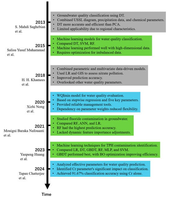
Figure 1.
Timeline of research work [12,13,14,15,16,17,18].
Table 1 provides an overview of various research studies that applied machine learning and statistical models for water quality classification and prediction. It includes details about the methodologies used, the specific algorithms and models applied, and main findings.

Table 1.
Summary of the main research content in the above studies.
- (1)
- Limitations of single model optimization: Many existing studies focus on enhancing the performance of single models by incorporating optimization algorithms. However, single models have inherent limitations when handling complex water quality data, particularly regarding feature selection and the modeling of nonlinear relationships, challenges that optimization algorithms alone cannot fully address. While some research has explored improving model performance through ensemble learning methods, there is a limited exploration of combining GBDT and MLP models specifically for water quality classification.
- (2)
- Lack of dynamic feature selection mechanisms: Most current water quality classification models depend on static feature weights, making them unable to dynamically adjust the importance of features according to different tasks or environmental conditions. This limits the model’s adaptability in handling complex and changing water quality monitoring tasks. In particular, there is a weak correlation between water quality characteristics and labels.
- (3)
- Parameter selection and simplification: To enhance computational efficiency, some studies reduce water quality parameters to simplify model structures. However, this simplification strategy may overlook key water quality features, reducing classification accuracy. While simplifying models can reduce computational burdens, it may also weaken overall model performance under complex water quality conditions, particularly when significant interactions between multiple parameters are present, leading to the potential omission of critical water quality information and impacting classification outcomes.
While these studies have made progress in water quality classification across different regions, several key issues remain:
In response to these issues, this study proposes an innovative solution by constructing a hybrid model, BS-MLP, which combines the strengths of GBDT for feature selection and the power of MLP in handling nonlinear relationships. Through this ensemble learning approach, the model can effectively capture complex feature interactions in water quality data, addressing the limitations of single models when dealing with intricate data. Additionally, we introduced a self-constructed feature-weighted attention mechanism in the BS-MLP model, resulting in the BS-FAMLP model. This mechanism dynamically adjusts the weights of different features, enabling the model to flexibly select features based on varying tasks or environments. Compared to traditional static feature weighting, the feature-weighted attention mechanism can dynamically identify and focus on the most critical features according to the specific water quality data, thereby improving the model’s generalization and classification accuracy. Lastly, we adopted a comprehensive strategy for parameter selection, retaining as many water quality features as possible to prevent the loss of crucial information. Through the dual innovations of the hybrid model and dynamic feature-weighting mechanism, we achieve both computational efficiency and model accuracy, ensuring high classification performance even in complex water quality environments or when dealing with imbalanced datasets.
Key parameter data from water quality samples are obtained through sensors or other technological means and input into the BS-FAMLP model, which can automatically output classification labels for the water samples. This innovative water quality classification model significantly simplifies the cumbersome laboratory analysis process, greatly enhances efficiency, and effectively reduces costs, providing substantial convenience and economic benefits for water resource management and protection efforts.
2. Materials and Methods
This section introduces the datasets used in this paper, describes the machine learning methods adopted, and provides the evaluation criteria for the models. Figure 2 shows the methodological process followed in this article.
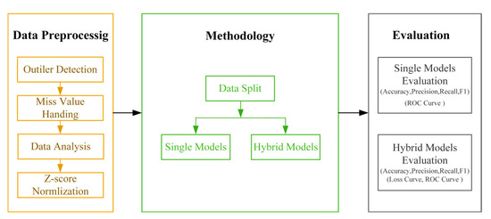
Figure 2.
The methodological process followed in this article.
2.1. Data Sources and Description
The dataset we used is a public dataset provided by the European Environment Agency and the World Bank. This dataset covers groundwater quality samples from multiple countries and regions. Each sample includes 15 water quality parameters that measure various aspects of water quality. The determination of water quality typically relies on multiple chemical and physical parameters that directly affect the safety and suitability of the water body. Chemical parameters, such as pH, dissolved oxygen, concentrations of nitrogen and phosphorus, and heavy metal content, can reflect the degree of pollution and nutrient status of the water. For example, pH influences the reactivity of chemical reactions in the water, while dissolved oxygen is a critical factor for the survival of aquatic organisms. Physical parameters, such as turbidity, temperature, and conductivity, also significantly impact water quality. Turbidity serves as an indicator of suspended solids in water, with higher turbidity potentially indicating pollution, while conductivity reflects the concentration of ions in the water. A comprehensive analysis of these parameters can provide a scientific basis for water quality assessment, helping to identify water quality issues and formulate appropriate remediation measures.
The detailed description is as follows:
- pH: indicates the acidity or alkalinity of the water.
- Turbidity: measures the amount of suspended solids in water, serving as an indicator of waste disposal.
- Dissolved solids: used to measure the ability of water to dissolve various organic and organic minerals.
- Chloramine: represents the concentration of chloramine, a primary disinfectant.
- Conductivity: reflects the water’s electrical conductivity, which increases with ion concentration.
- Nitrates, sulfates, chlorides, fluorides: indicate the concentrations of these substances in water.
- Various metals: indicate the levels of metal elements in the water sample.
Each sample has classification labels of “Safe” and “Unsafe”, represented by 1 and 0, respectively. These labels indicate whether the water samples meet drinking water standards. The dataset comprises a total of 188,623 samples, with 80,948 samples labeled as 1 (Safe) and 107,675 samples labeled as 0 (Unsafe).
2.2. Machine Learning Algorithms
The core research focus of this paper is to develop a machine learning model to classify water samples using the obtained water quality parameter data, replacing traditional laboratory analysis processes. To gain a deeper understanding of this process, we will briefly introduce the machine learning classification algorithms employed in this study.
2.2.1. Single Models
- 1.
- Adaptive Boosting (ADA)
ADA is an ensemble learning method. It combines multiple weak classifiers to build a strong classifier to improve classification accuracy. The core principle of ADA is the sequential training of classifiers, each weak classifier focusing on the misclassified samples from the previous round. This process involves adjusting sample weights to prioritize difficult-to-classify instances. ADA aggregates the results of these classifiers to form a robust model that enhances overall accuracy [19]. The mathematical process of the ADA model is as follows.
Step 1: Initialize weights. For each sample i, initialize the weight as
where N is the total samples.
Step 2: Calculate classifier error rate.
where I(⋅) is an indicator function that takes the value 1 if the prediction is incorrect, and 0 otherwise.
Step 3: Compute classifier weight:
Step 4: Update sample weights.
The final classifier is a weighted sum of weak classifiers.
- 2.
- Logistic Regression (LR)
Logistic regression is a robust and versatile classification algorithm. It uses a logical function to obtain the probability that a sample belongs to a specific category. The goal of logistic regression is to maximize the likelihood function to determine the optimal feature weights. Despite its name, logistic regression is primarily used for classification, particularly for linearly separable data [20,21].
Model’s linear equation:
The logistic function (sigmoid) transforms the linear output into probability.
Loss function:
- 3.
- Gaussian Naive Bayes (GNB)
Gaussian naive Bayes is a classification algorithm based on Bayes’ theorem. For continuous features, GNB assumes that these features follow a Gaussian distribution. It calculates the conditional probability of each feature for each category and combines these probabilities using Bayesian formulas to derive the posterior probability of a sample belonging to a specific class. Although the assumption of feature independence often does not hold, GNB performs well in many real-world applications, particularly with high-dimensional data and multi-category classification problems [22].
For each feature assuming Gaussian distribution,
where and are the mean and variance of feature in class .
Use Bayes’ theorem to compute posterior probability.
Final predicted class:
- 4.
- K-Nearest Neighbors (KNNs)
KNNs is an instance-based classification model. It classifies samples by measuring the distance between the sample to be classified and the samples in the training set. For each sample, KNNs identifies its K closest neighbors and classifies the sample based on the majority class of these neighbors. KNNs is known for its simplicity and intuitive nature, but it can be computationally expensive with large datasets and sensitive to noisy data [23].
Step 1: Calculate the distance between test sample x and training sample .
where n is the number of features, is the feature of the test sample x, and is the feature of the training sample .
Step 2: Select K nearest neighbors and classify based on majority vote.
where denotes the set of K nearest neighbors of x, is the class label of the neighbor, and I(⋅) is the indicator function, which is 1 if equals k, and 0 otherwise. The argument selects the class k with the highest count among the neighbors.
- 5.
- Support Vector Machine (SVM)
SVM is an algorithm based on decision boundaries that seeks to separate different classes of data by finding an optimal hyperplane in a high-dimensional space. The objective of SVM is to maximize the margin between classification boundaries, i.e., the minimum distance between support vectors and the hyperplane. By utilizing kernel functions, SVM can handle nonlinearly separable data, enhancing the model’s ability to generalize, particularly in high-dimensional and complex classification tasks [24,25].
For linearly separable data, the SVM aims to find the optimal separating hyperplane defined by
where w is the normal vector to the hyperplane, and b is the bias.
Maximize margin γ equivalent to minimizing objective function.
subject to constraints
If data are not linearly separable, use the kernel function to map data to higher-dimensional space. Common kernel functions include
where is the squared Euclidean distance between samples, and . σ is a parameter that controls the width of the Gaussian function.
- 6.
- Gradient Boosting Decision Tree (GBDT)
GBDT is an ensemble learning algorithm that builds multiple decision trees through iterative processes. The algorithm combines decision trees with an ensemble approach, with the basic decision tree model selected from Classification Regression Trees (CARTs). The initial decision tree is generated using the original data features. Subsequent trees are created to minimize the aggregate loss function from previous trees, continuing until the loss function converges to zero. The final classification results are obtained by linearly weighting the outputs of all decision trees [26,27,28].
Specific algorithmic steps of the GBDT model are as follows:
Input: Training set , where .
Output: Regression tree .
(1) Initialize the weak classifier.
where is the initial decision tree; is the loss function; and c is the constant that satisfies the minimum of the loss function.
(2) For iterations.
① Calculate the negative gradient of samples.
② Construct a decision tree Tm using all samples and their negative gradient directions , with J leaf nodes and regions Rmj corresponding to each leaf node.
③ Compute the best-fit values for the J leaf nodes of Tm.
④ Update the classifier for this iteration.
(3) Obtain the formula for the final decision tree.
- 7.
- Multi-Layer Perceptron (MLP)
MLP is a type of artificial neural network used extensively in classification problems and big data analytics. It captures complex patterns and features by nonlinearly transforming input data through multiple layers of neurons. MLP can solve nonlinearly separable problems by incorporating hidden layers and nonlinear activation functions [29]. An MLP is a network of multiple perceptrons, each of which is a simple linear classifier. By stacking multiple such layers, an MLP can learn complex nonlinear relationships from input data [30].
Forward Propagation (FP):
where is the linear combination output of the first hidden layer; is the weight matrix from the input layer to the first hidden layer; is the bias vector of the first hidden layer; and is the activation output of the first hidden layer.
Layer l to layer l + 1 (l = 1, 2,…, l − 1):
Each neuron performs a weighted sum of the input, followed by the application of an activation function. The output passes through all hidden layers to the output layer, which generates the model’s classification probability.
where is the linear combination output of the last hidden layer; is the weight matrix from the last hidden layer to the output layer; is the bias vector of the output layer; and is the predicted probability vector.
In this paper, we add the cross-entropy loss function to the model.
where C is the number of categories; is the one-hot coding of the actual categories; and is the predicted probability.
Backpropagation:
Output layer error:
where is the error in the output layer; is the one-hot coding of the actual label; is the error in the lth layer; and is the derivative of the ReLU function.
Calculate the weight gradient and bias gradient, respectively, according to the following equations:
where is the gradient of the loss function with respect to the weight of the th layer and is the gradient of the loss function with respect to the bias of the th layer.
Weight and bias updates:
Table 2 shows the parameters used in the classification algorithm in the text.

Table 2.
Hyperparameter settings [19,20,21,22,23,24,25,26,27,28,29,30].
2.2.2. BS-FAMLP Hybrid Model Building
GBDT and MLP each offer distinct advantages. GBDT excels at capturing complex relationships between features when processing structured data and is highly robust against outliers and noise. However, it can be prone to overfitting when handling high-dimensional data or complex nonlinear patterns. On the other hand, MLP, with its multiple layers of nonlinear transformations, can uncover intricate patterns within the data, performing exceptionally well on high-dimensional and large-scale datasets. By combining these strengths, GBDT can serve as a feature extractor, while MLP further processes these features for classification, leading to a significant boost in overall model performance.
Within the ensemble learning framework, this paper introduces a hybrid model, BS-MLP, combining GBDT [26] and MLP [31]. To further enhance model performance, we dynamically adjust the weights of water quality feature parameters to improve the model’s focus on key features and minority samples. A feature-weighted attention mechanism is designed and integrated into the BS-MLP model, resulting in the construction of the BS-FAMLP model.
The feature-weighted attention mechanism works as follows:
Feature input: In the Stacking layer, the output of the GBDT model each sample belongs to is the probability value of class 1 samples. We form a new feature vector with these probability values along with the actual labels of the samples as input to the final MLP. The new feature vector can be expressed as .
Calculation of feature weights. The attention score formula is as follows:
where is the hidden state at the current moment; is the state at the previous moment; and are the weight matrices; v is the weight vector; and is the bias vector.
Subsequently, the attention weights are calculated by the SoftMax function
where is the attention weight at the moment.
Feature weighting: the computed weights are applied to the original feature x to generate a new weighted feature vector x′.
where ⊙ denotes element-by-element multiplication. The weighted feature vector x′ reflects the importance of different features for the classification task.
Feature weighting adjustment: in order to prevent the model from relying too much on certain features, especially in unbalanced datasets that may affect the classification effect of a few classes of samples, we introduce a category-sensitive adjustment mechanism. If the contribution of a feature to two classes of samples is the same, the weight of the feature is reduced. The adjusted feature weights make the model more robust in categorizing minority class samples and prevent the model from deviating from the actual goal due to noise or unimportant features.
Aggregated output: the weighted feature vector x′ is input to the subsequent classifier MLP for final prediction. The output of the MLP is passed to the cross-entropy loss cost function. The model gradually improves its accuracy for the classification task by optimizing this loss function.
Finally, the BS-FAMLP model features two layers of GBDT and an MLP model with a feature-weighted attention mechanism, as illustrated in Figure 3.
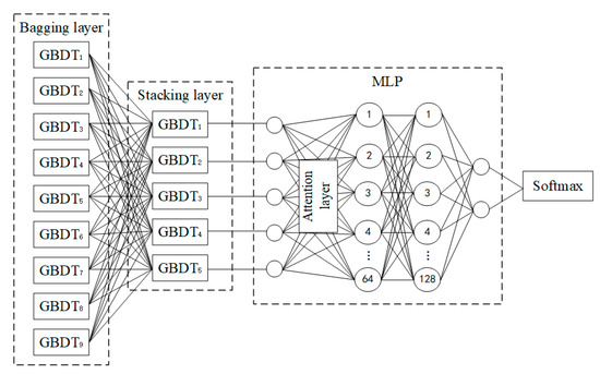
Figure 3.
Structure of the BS-FAMLP model.
According to the Stacking framework and ensemble learning theory, several independent GBDT models are established [32]. The proposed method uses two GBDT layers, namely the Bagging layer and the Stacking layer, with the number of GBDT models in each layer determined by grid search cross-validation. The Bagging layer consists of 9 GBDT models, taking the feature vector X of the data sample as input and outputting the probability of the sample as class 1. The Stacking layer comprises 5 GBDT models, using the 9 probabilities from the Bagging layer to form a new feature vector X′ for input, producing similar outputs to the Bagging layer.
The MLP component contains an Input layer, two hidden layers, and an output layer. The input layer has 5 neurons and receives the output from the last GBDT layer. The first hidden layer and the second hidden layer contain 64 and 128 neurons, respectively. The neuron activation function is ReLU. The output layer consists of a fully connected layer and a Softmax layer.
2.3. Model Evaluation Criteria
To distinguish between the classification performance of the models, several metrics were selected: Accuracy, Precision, Recall, F1 Score, and AUC [33].
- 1.
- Accuracy
Measures the proportion of correctly predicted results among the total predictions, calculated as [34]
- 2.
- Precision
Precision is mainly used to assess how many positive samples are actually positive samples. The value of the Precision rate is between 0 and 1. The larger this value, the more accurate the model in predicting positive examples [34,35].
- 3.
- Recall
Recall rate is mainly used to measure how many true positive examples are covered by the model. The value of the Recall rate has a range of [0, 1]. The higher the value, the more the model covers the positive examples [34,35].
- 4.
- F1 Score
The F1 Score is the reconciled average of precision and recall, which is mainly used to measure the effectiveness of the classification model [34,35]. In some cases, such as when the number of positive and negative class samples is extremely unbalanced, the F1 Score is a better reflection of the model’s effectiveness than Precision and Recall.
- 5.
- AUC
The ROC curve calculates a series of False Positive Rate (FPR) and True Positive Rate (TPR) points by shifting the classification thresholds from high to low and then drawing the curve on the FPR and TPR axes [33]. The AUC value has a range of [0, 1]. The larger the AUC, the better the model’s predictive effect. When the AUC is equal to 0.5, the model’s predictive effect is equivalent to random guessing.
3. Experiments
3.1. Hardware and Software Configuration
The hardware and software configuration for this study is detailed in Table 3.

Table 3.
Computer environment for training and testing machine learning models.
3.2. Dataset Description and Preprocessing
3.2.1. Data Preprocessing
Outliers can significantly affect model training by distorting data distribution, decreasing accuracy, and leading to incorrect conclusions. Therefore, addressing outliers is essential in data preprocessing to ensure reliable analysis and interpretable models [36]. In this paper, a box-and-line plot is used to detect outliers, where the two ends of the box correspond to the lower quartile Q1 and the upper quartile Q3, and the interval between Q1 and Q3 is called the inter-quartile range (IQR). The upper and lower cutoffs of the outliers are the points corresponding to the positions of three-times the IQR outside the quartiles, respectively. Data outside of (Q3 + 3IQR, and Q1 − 3IQR) are considered outliers. The outlier detection box-and-line diagram is shown in Figure 4. We replace all the identified outliers with null values and process them in the next step.
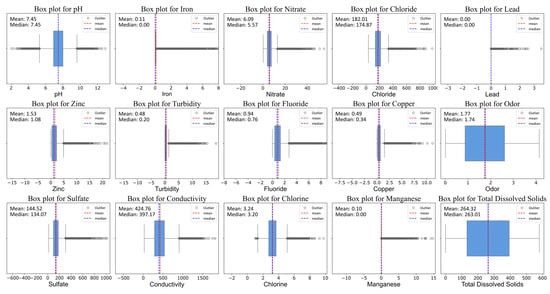
Figure 4.
Use a box plot to detect outliers in the water quality parameters of a dataset.
Missing values can lead to incomplete data and affect experiment accuracy. Complete data can provide more comprehensive information for scientific research and decision-making, so dealing with missing values is an important issue after identifying outliers. Table 4 shows the missing values in the dataset.

Table 4.
Number of missing values for the water quality parameters in the dataset.
As shown in Table 4, copper has the most missing values in the water quality sample data, while total dissolved solids has the fewest. Additionally, chloride, fluoride, odor, sulfate, and conductivity also have a relatively high number of missing values.
Two common methods for handling missing values are direct deletion and interpolation. Direct deletion avoids introducing bias and preserves the original data distribution but results in a reduction of sample size. Conversely, interpolation maintains the sample size but may introduce additional noise or bias depending on the interpolation method used. To leverage the benefits of both methods while minimizing their drawbacks, this study employs the K-nearest neighbors (KNNs) imputation technique for handling missing values in the water quality dataset. To account for the differences in the physical scales of various chemical components and improve the accuracy of imputation, the Manhattan distance was chosen as the metric to calculate the distance between samples. During the imputation process, for each sample with missing values, we calculated the Manhattan distance between it and the samples without missing values, selecting k most similar (nearest neighbor) samples. The mean of these neighbors for the corresponding features was then used for imputation. This method effectively preserved the relative differences between water quality features, ensuring the integrity of the data structure. The imputation covered not only the original missing values but also the outliers that were replaced by null values during outlier handling. By selecting different values of k for the imputation, a total of 40 datasets were generated.
3.2.2. Evaluation of Data Preprocessing
To systematically evaluate the impact of data preprocessing, we trained a random forest model on both the original dataset and the 40 preprocessed datasets [37]. The evaluation metrics used are the root mean square error (RMSE), mean absolute error (MAE), and the coefficient of determination (R2) [38]. Figure 5 demonstrates the trend in preprocessing effectiveness. The optimal imputation effect was observed with K = 15.
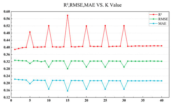
Figure 5.
RMSE, MAE, and R2 after filling with different values of K.
The dataset imputed using the KNN method with K = 15 outperforms the original dataset across all evaluation metrics. As shown in Table 5, compared to the original dataset, the RMSE is reduced by 0.046, the MAE is reduced by 0.064, and the R2 is improved by 0.186. These improvements indicate that the preprocessing step significantly enhances data quality, thereby providing a more reliable basis for subsequent model training and prediction.

Table 5.
The prediction results of the random forest on the original dataset and the dataset after data preprocessing.
3.2.3. Data Analysis
Table 6 shows the mean, maximum, and minimum values for the best-populated dataset, as well as the World Health Organization standards for each component of potable water quality. These data provide a reference for further classification of water quality.

Table 6.
WHO limits for various water quality parameters and some statistical values.
3.2.4. Data Distribution Analysis
After preprocessing, the dataset was prepared for model training and testing. To understand the data characteristics and potential issues, data distribution histograms were reviewed, as shown in Figure 6. The results reveal that most features (e.g., nitrate, chloride, zinc, turbidity) exhibit a right-skewed distribution. Some features (e.g., pH, chlorine) are approximately normally distributed, while others (e.g., odor, total dissolved solids) display a more uniform distribution.
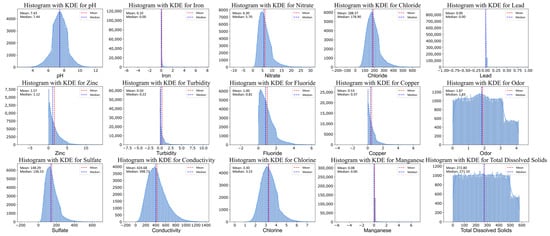
Figure 6.
Histogram of the data distribution to observe the distribution of water quality parameters in the dataset.
The final dataset used for model training includes 188,623 samples, of which 80,948 are labeled as 1 and 107,675 are labeled as 0.
3.2.5. Correlation Analysis
In this study, we used Formula (44) to calculate the correlation coefficient between the characteristic parameters and the dependent variable. The Pearson correlation coefficient can reflect the linear correlation between two variables and takes on values between [−1, 1]. The calculation formula is
Additionally, to visually present the correlations between the parameters and between the parameters and the labels, a heatmap was used for visualization [39]. We describe the strength of the correlation according to the meaning of the Pearson coefficient shown in Table 7.

Table 7.
Interpretation of the physical meaning of the Pearson coefficient (r) [40].
Figure 7 illustrates these correlations, showing that most feature correlations are very weak, with coefficients near zero.
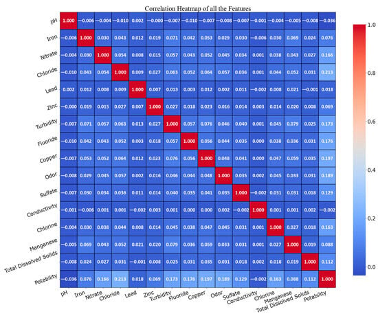
Figure 7.
Heatmap of the correlation between water quality features and labels.
Particularly, Table 8 shows the correlation between individual features and labels.

Table 8.
Correlation between features and labels.
This table indicates that while there is some correlation between sample characteristics and labels, most characteristics exhibit a positive correlation with the labeled values. This suggests that these characteristics may influence the drinkability of water, with few significant negative correlations.
3.3. Data Normalization
To address numerical biases and ensure that features with different scales do not adversely affect each other, the data were normalized [41]. The normalization formula used is
4. Results and Discussion
4.1. Single Model Classification Results
We initially evaluated various single classification algorithms on the dataset, and the results are summarized in Table 9.

Table 9.
Classification results of the single model on the test set.
Overall, the classification accuracies for all models exceeded 0.6, indicating that that the models can classify the samples to a certain extent, performing better than random guessing. However, this also shows that there is still much room for improvement in the models’ performance. Among these, the GBDT model demonstrated the best performance across all evaluation metrics, significantly outperforming the other models. The MLP and SVM models also exhibited strong classification capabilities, though slightly less effective than GBDT. This suggests that the GBDT model is adept at capturing complex patterns in the data and providing high-quality classifications. We also plotted the ROC curves for each model, shown in Figure 8, to further illustrate their classification performance.
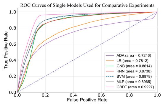
Figure 8.
ROC curve of a single model on the test set.
The ROC curves reveal that the GBDT model has the largest AUC, followed by MLP and SVM, with AUC values of 0.9277, 0.8965, and 0.8879. This indicates that these models have strong classification abilities for this dataset and can effectively differentiate between positive and negative class samples. The ADA model, however, performs relatively poorly, with an AUC of 0.7246, and its ROC curve is significantly distant from the upper left corner of the graph. The ADA model struggles with classification, likely due to data imbalance, causing it to focus excessively on the majority class and neglect the minority class samples.
Based on these results, we chose GBDT and MLP as the base learners for constructing the hybrid model, as they exhibited the best performance among the single models.
4.2. Classification Results of the Hybrid Model
4.2.1. Model Training
Figure 3 illustrates the network structure of the hybrid model proposed in this paper, which consists of three layers of learners. The training process is as follows:
In the first stage, we used the Bootstrap sampling technique in the Bagging method to create nine independent sub-datasets for training nine GBDT models. Each sub-dataset, containing 12,000 samples, was divided into training and validation sets in an 8:2 ratio. We optimized the hyperparameters of each GBDT model using Bayesian optimization to better approximate the probability of a sample being labeled as 1. Figure 9 shows the parameter optimization process for the GBDT models in the Bagging layer. Bayesian optimization improves both the learning ability and adaptability of the model to the dataset’s complexity.
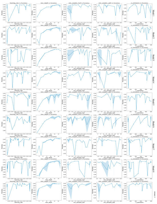
Figure 9.
Optimization process of GBDT model parameters in the Bagging layer.
In the second stage, we trained five GBDT models using the Stacking framework. For each water quality sample in the original training set, the nine GBDT models in the first layer output nine probability values. These values are stacked to form a new feature vector, which, along with sample labels, constitutes a new training set for the second layer. The second-layer GBDT models were trained using five-fold cross-validation. Figure 10 shows the optimization process for GBDT model parameters in the Stacking layer.
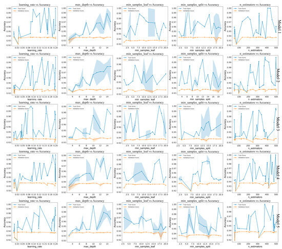
Figure 10.
Optimization process of GBDT model parameters in the Stacking layer.
In the third stage, we trained the MLP as the final-level learner using five-fold cross-validation. The MLP takes the outputs from the first two levels of the GBDT network as input features and is trained using a binary cross-entropy loss function with a regularization term. The parameters for each layer model are detailed in Table 10.

Table 10.
Parameters for each layer of the model.
To enhance model performance, we incorporated an autonomously constructed feature-weighted attention mechanism into the MLP model, resulting in the BS-FAMLP model.
Table 11 summarizes the results for each layer of the model on the test set. For the Stacking layer and MLP, the results are averaged over five-fold cross-validation.

Table 11.
Classification results of each layer model on the training set.
The data in the table show that classification performance improves progressively with each model layer, culminating in optimization at BS-FAMLP. In the Bagging layer, the GBDT models perform well across all evaluation metrics, especially in Recall and F1 Score, demonstrating their excellent performance in classification tasks. Their accuracies fluctuate between 0.89 and 0.91, indicating that Bagging’s randomness effectively enhances the model’s generalization ability. In the Stacking layer, the performance of the GBDT models is further improved through additional feature combinations from the Bagging layer outputs. All models maintain an accuracy around 0.936 and F1 Scores above 0.938, showing their capability to efficiently handle classification tasks. In the MLP layer, the integration of GBDT layer outputs leads to further optimization of feature nonlinearity, resulting in improved model performance. However, it is worth noting that despite improvements in accuracy and F1 Score, the Recall in the MLP layer decreases. This may be due to a greater emphasis on enhancing overall classification accuracy and precision during optimization, which can reduce the ability to identify samples from minority classes and lower sensitivity to true positive samples. These results indicate that each component contributes to performance gains, collectively enhancing overall model performance.
4.2.2. Ablation Study
Ablation study is a key technique for evaluating the impact of specific components or methods in a machine learning model. By systematically removing or modifying a part of the model, the contribution of each component to the overall performance is revealed. In this study, five sets of experiments were designed to evaluate the classification performance of different models. These experiments include the following:
- (1)
- Model B-MLP with the hybrid of two learners, Bagging layer and MLP.
- (2)
- Model BS-MLP with three learners fused.
- (3)
- Model BS-FAMLP with feature-weighted attention mechanism added to the BS-MLP model.
- (4)
- Model BS-SAMLP that adds a self-attention mechanism to the BS-MLP model.
- (5)
- Model BS-MAMLP that adds a multi-head attention mechanism to the BS-MLP model.
The above five models were cross-validated on the training set using five-fold cross-validation, and the training results are shown in Table 12.

Table 12.
Classification results of the hybrid model on the test set (five-fold).
From the table, it is evident that all models exhibit strong classification performance on the training set. The average accuracies of the base models B-MLP and BS-MLP on the training set are 0.9371 and 0.9435, respectively. BS-MLP outperforms B-MLP, indicating that the introduction of the Stacking layer effectively enhances classification performance. The inclusion of attention mechanisms further improves the model’s average accuracy, reaching 0.9629, 0.9546, and 0.9642, respectively. This demonstrates that adding different types of attention mechanisms significantly enhances classification performance. However, it is important to note that the training time for models with attention mechanisms increases substantially. Compared to the base model, the training times for BS-FAMLP, BS-SAMLP, and BS-MAMLP models increased by approximately seven, five, and thirty times, respectively.
In summary, the structural complexity of the models and the enhancement of feature extraction methods significantly impact classification performance. While the introduction of attention mechanisms greatly improves model performance, it also leads to longer training times. Among these, the BS-MAMLP model shows the most significant performance improvement, though it also has the longest training time. On the other hand, the BS-FAMLP model, with its autonomously constructed feature-weighted attention mechanism, demonstrates a notable advantage in classification performance. Although BS-FAMLP slightly trails behind BS-MAMLP in terms of performance, its training time is reduced by about six times, achieving a better balance between performance and computational efficiency. Compared to BS-SAMLP, BS-FAMLP not only improves classification performance but also manages a slight increase in training time.
4.2.3. Test Set Performance Evaluation
The classification results of the five models on the test set are shown in Table 13.

Table 13.
Classification results of the layer model on the test set.
The data show that the classification performance of the five models aligns with their performance on the training set. The base B-MLP model offers better classification results, but the BS-MLP model, with stacked layers, improves all performance metrics. This suggests that additional GBDT layers better capture complex features in the data. The introduction of a feature-weighted attention mechanism in the BS-MLP model significantly improves all performance metrics, highlighting the crucial role of attention mechanisms in enhancing model accuracy and robustness. Further, Figure 11 illustrates the loss function curves for each model.
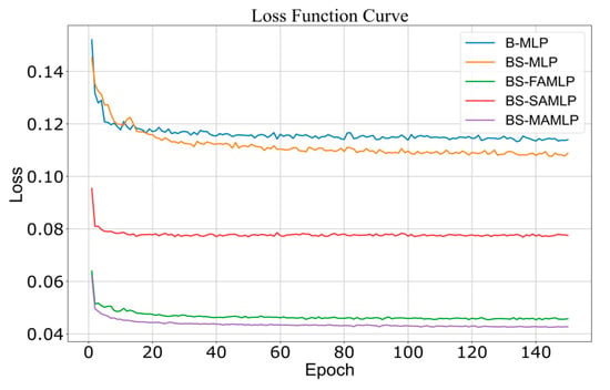
Figure 11.
Loss function curve of each hybrid model on the test set.
The figure shows that the loss function values of all models decrease gradually with training batches, indicating that the models adapt to the data and improve their performance during training. The base model B-MLP starts with a high loss value but quickly drops to around 0.11 with increasing training batches. The BS-MLP model has a lower loss value compared to B-MLP. Both BS-FAMLP and BS-MAMLP models exhibit a similar decreasing trend in loss values and maintain lower loss values. The BS-SAMLP model declines faster but has higher loss values compared to BS-FAMLP and BS-MAMLP.
Additionally, Figure 12 presents the ROC curves for the five models, further visualizing differences in model performance.

Figure 12.
ROC curve of each hybrid model on the test set.
The figure shows that the AUC value of the BS-FAMLP model reaches 0.9834, second only to the 0.9875 of the BS-MAMLP model. This indicates that BS-FAMLP performs very well in terms of categorization accuracy and effectively distinguishes between categories. Models with attention mechanisms perform significantly better than the base models, with the AUC values for BS-MAMLP and BS-SAMLP being 0.9610 and 0.9715, respectively.
These results further confirm that the autonomously constructed feature-weighted attention mechanism in the BS-FAMLP model not only improves classification performance but also demonstrates better generalization ability on the test set.
5. Conclusions
This study aims to develop an efficient and reliable machine learning model for water quality classification. The model assesses the safety of water quality by analyzing the obtained water quality parameter data, thereby replacing the cumbersome, inefficient, and costly laboratory analysis processes of traditional methods. Initially, through the performance evaluation of six individual models, we found that the GBDT model performed the best on the test set, with an accuracy of 0.8719 and an AUC value of 0.9277, while the MLP and SVM models also demonstrated good results. Based on this, the proposed BS-FAMLP hybrid model was further validated through ablation and comparison experiments.
The ablation experiments showed that as the model’s complexity increased, its classification performance gradually improved, particularly after introducing the feature-weighted attention mechanism, where the model’s accuracy increased from 0.94 to 0.96. The comparison experiments revealed that the BS-MAMLP model slightly outperformed BS-FAMLP in classification performance, with an accuracy of 0.9632 and an AUC value of 0.9608 on the test set. However, this came at the cost of significantly longer training times. In contrast, the BS-FAMLP model achieved an accuracy of 0.9616 and an AUC value of 0.9589, with only one-sixth of the training time required by BS-MAMLP.
One of the key innovations in this study is the independently developed feature-weighted attention mechanism. By using this mechanism, the model dynamically adjusts the importance of features, thereby improving its performance. This approach allows the model to automatically learn which features are more important for a given task, enhancing its predictive ability. This is particularly beneficial in handling imbalanced datasets, as it helps the model better focus on important features of minority class samples.
There is still room for improvement despite the significant achievements of the methods proposed in this paper:
- Parameter Optimization and Algorithm Selection: Explore more efficient optimization algorithms to prevent local optima and enhance model performance.
- Data Preprocessing: Adopt more advanced missing value imputation and outlier detection techniques to improve data integrity and reliability.
- Imbalanced Data Handling: Use ensemble learning or generative adversarial networks (GANs) to increase minority class samples and improve classification performance.
- Model Lightweighting: Simplify the model structure to increase operational efficiency, making it easier to deploy in resource-constrained environments for real-time classification.
These improvement directions aim to enhance the model’s accuracy, generalization ability, and practicality, making it more advantageous in real-world applications. Overall, the proposed BS-FAMLP model demonstrates the ability to accurately and efficiently classify water quality samples, effectively addressing the shortcomings of traditional machine learning in water quality assessment. The research results indicate that this model has the potential to replace laboratory analysis, providing a more convenient and cost-effective solution for water quality monitoring and management.
Author Contributions
This research was jointly performed by W.C., D.X., B.P., Y.Z. and Y.S. All authors of the article made the same contribution. All authors have read and agreed to the published version of the manuscript.
Funding
This research was funded by the Liaoning Provincial Natural Science Foundation Project, Industrial Internet Logo Data Association Relationship Based on Machine Online Learning relationship analysis, grant number 2022-KF-12-11.
Data Availability Statement
The dataset used in this article can be accessed through Kaggle at https://www.kaggle.com/datasets/water potability prediction (accessed on 2 May 2023).
Conflicts of Interest
Duo Xu was employed by Shenyang Ceprei Technology Service Co., Ltd., Bowen Pan was employed by Liaoshen Industries Group Co., Ltd., and Yuan Zhao was employed by Shipbuilding Equipment and Materials Northeast (China) Co., Ltd. The remaining authors declare that the research was conducted in the absence of any commercial or financial relationships that could be construed as a potential conflict of interest..
References
- Kumar, P. Simulation of Gomti River (Lucknow City, India) future water quality under different mitigation strategies. Heliyon 2018, 4, 1074. [Google Scholar] [CrossRef] [PubMed]
- Ahmed, J.; Wong, L.P.; Chua, Y.P.; Channa, N.; Mahar, R.B.; Yasmin, A.; VanDerslice, J.A.; Garn, J.V. Quantitative Microbial Risk Assessment of Drinking Water Quality to Predict the Risk of Waterborne Diseases in Primary-School Children. Int. J. Environ. Res. Public Health 2020, 17, 2774. [Google Scholar] [CrossRef]
- Tleuova, Z.; Snow, D.D.; Mukhamedzhanov, M.; Ermenbay, A. Relation of hydrogeology and contaminant sources to drinking water quality in southern Kazakhstan. Water 2023, 15, 4240. [Google Scholar] [CrossRef]
- Zhu, M.; Wang, J.; Yang, X.; Zhang, Y.; Zhang, L.; Ren, H.; Wu, B.; Ye, L. A review of the application of machine learning in water quality evaluation. Eco-Environ. Health 2022, 1, 107–116. [Google Scholar] [CrossRef] [PubMed]
- Mahgoub, H.A. Extraction techniques for determination of polycyclic aromatic hydrocarbons in water samples. Int. J. Sci. Res. 2013, 1, 268–272. [Google Scholar]
- Hu, C.; Dong, B.; Shao, H.; Zhang, J.; Wang, Y. Toward purifying defect feature for multilabel sewer defect classification. IEEE Trans. Instrum. Meas. 2023, 72, 5008611. [Google Scholar] [CrossRef]
- Kang, J.-K.; Lee, D.; Muambo, K.E.; Choi, J.-W.; Oh, J.-E. Development of an embedded molecular structure-based model for prediction of micropollutant treatability in a drinking water treatment plant by machine learning from three years monitoring data. Water Res. 2023, 239, 120037. [Google Scholar] [CrossRef]
- Uddin, M.G.; Nash, S.; Rahman, A.; Olbert, A.I. Performance analysis of the water quality index model for predicting water state using machine learning techniques. Process Saf. Environ. Prot. 2023, 169, 808–828. [Google Scholar] [CrossRef]
- Muharemi, F.; Logofătu, D.; Leon, F. Machine learning approaches for anomaly detection of water quality on a real-world data set. J. Inf. Telecommun. 2019, 3, 294–307. [Google Scholar] [CrossRef]
- Pedro-Monzonís, M.; Solera, A.; Ferrer, J.; Estrela, T.; Paredes-Arquiola, J. A review of water scarcity and drought indexes in water resources planning and management. J. Hydrol. 2015, 527, 482–493. [Google Scholar] [CrossRef]
- Memon, A.G.; Mustafa, A.; Raheem, A.; Ahmad, J.; Giwa, A.S. Impact of effluent discharge on recreational beach water quality: A case study of Karachi-Pakistan. J. Coast. Conserv. 2021, 25, 37. [Google Scholar] [CrossRef]
- Saghebian, S.M.; Sattari, M.T.; Mirabbasi, R.; Pal, M. Ground water quality classification by decision tree method in Ardebil region, Iran. Arab. J. Geosci. 2013, 7, 4767–4777. [Google Scholar] [CrossRef]
- Muhammad, S.Y.; Makhtar, M.; Rozaimee, A.; Aziz, A.A.; Jamal, A.A. Classification model for water quality using machine learning techniques. Int. J. Softw. Eng. Appl. 2015, 9, 45–52. [Google Scholar] [CrossRef]
- Rizeei, H.M.; Azeez, O.S.; Pradhan, B.; Khamees, H.H. Assessment of groundwater nitrate contamination hazard in a semi-arid region by using integrated parametric IPNOA and data-driven logistic regression models. Environ. Monit. Assess. 2018, 190, 633. [Google Scholar] [CrossRef] [PubMed]
- Nong, X.; Shao, D.; Zhong, H.; Liang, J. Evaluation of water quality in the South-to-North Water Diversion Project of China using the water quality index (WQI) method. Water Res. 2020, 178, 115781. [Google Scholar] [CrossRef]
- Nafouanti, M.B.; Li, J.; Mustapha, N.A.; Uwamungu, P.; AL-Alimi, D. Prediction on the fluoride contamination in groundwater at the Datong Basin, Northern China: Comparison of random forest, logistic regression and artificial neural network. Appl. Geochem. 2021, 132, 105054. [Google Scholar] [CrossRef]
- Huang, Y.; Ding, L.; Liu, W.; Niu, H.; Yang, M.; Lyu, G.; Lin, S.; Hu, Q. Groundwater contamination site identification based on machine learning: A case study of gas stations in China. Water 2023, 15, 1326. [Google Scholar] [CrossRef]
- Chatterjee, T.; Gogoi, U.R.; Samanta, A.; Chatterjee, A.; Singh, M.K.; Pasupuleti, S. Identifying the Most Discriminative Parameter for Water Quality Prediction Using Machine Learning Algorithms. Water 2024, 16, 481. [Google Scholar] [CrossRef]
- Singh, Y.; Walingo, T. Smart Water Quality Monitoring with IoT Wireless Sensor Networks. Sensors 2024, 24, 2871. [Google Scholar] [CrossRef]
- Hosmer, D.W.; Lemeshow, S.; Sturdivant, R.X. Applied Logistic Regression; John Wiley Sons: Hoboken, NJ, USA, 2013. [Google Scholar]
- Guns, M.; Vanacker, V. Logistic regression applied to natural hazards: Rare event logistic regression with replications. Nat. Hazards Earth Syst. Sci. 2012, 12, 1937–1947. [Google Scholar] [CrossRef]
- Zhang, H. The optimality of naive Bayes. In The Florida AI Research Society, Proceedings of the Seventeenth International Florida Artificial Intelligence Research Society Conference (FLAIRS 2004), Miami Beach, FL, USA, 12–14 May 2004; The AAAI Press: Menlo Park, CA, USA, 2004; ISBN 978-1-57735-201-3. [Google Scholar]
- Beyer, K.; Goldstein, J.; Ramakrishnan, R.; Shaft, U. When is “nearest neighbor” meaningful? In Proceedings of the International Conference on Database Theory, Jerusalem, Israel, 10–12 January 1999; pp. 217–235. [Google Scholar]
- Tong, S.; Koller, D. Support vector machine active learning with applications to text classification. J. Mach. Learn. Res. 2001, 2, 45–66. [Google Scholar]
- Zhang, H.; Zou, Q.; Ju, Y.; Song, C.; Chen, D. Distance-based support vector machine to predict DNA N6-methyladenine modification. Curr. Bioinform. 2022, 17, 473–482. [Google Scholar] [CrossRef]
- Friedman, J.H. Stochastic gradient boosting. Comput. Stat. Data Anal. 2002, 38, 367–378. [Google Scholar] [CrossRef]
- Huang, P.; Wang, L.; Hou, D.; Lin, W.; Yu, J.; Zhang, G.; Zhang, H. A feature extraction method based on the entropy-minimal description length principle and GBDT for common surface water pollution identification. J. Hydroinform. 2021, 23, 1050–1065. [Google Scholar] [CrossRef]
- Liang, W.; Luo, S.; Zhao, G.; Wu, H. Predicting hard rock pillar stability using GBDT, XGBoost, and LightGBM algorithms. Mathematics 2020, 8, 765. [Google Scholar] [CrossRef]
- Lin, H.-Y.; Lee, S.-H.; Wang, J.-H.; Chang, M.-J. Utilizing Artificial Intelligence Techniques for a Long–Term Water Resource Assessment in the ShihMen Reservoir for Water Resource Allocation. Water 2024, 16, 2346. [Google Scholar] [CrossRef]
- Günther, F.; Fritsch, S. Neuralnet: Training of neural networks. R J. 2010, 2, 30–38. [Google Scholar] [CrossRef]
- Pinkus, A. Approximation theory of the MLP model in neural networks. Acta Numer. 1999, 8, 143–195. [Google Scholar] [CrossRef]
- Zhou, Z.H. Ensemble Methods: Foundations and Algorithms; CRC Press: Boca Raton, FL, USA, 2012. [Google Scholar]
- McLaughlin, D.B. Assessing the predictive performance of risk-based water quality criteria using decision error estimates from receiver operating characteristics (ROC) analysis. Integr. Environ. Assess. Manag. 2012, 8, 674–684. [Google Scholar] [CrossRef]
- Sokolova, M.; Japkowicz, N.; Szpakowicz, S. Beyond Accuracy, F-Score, and ROC: A Family of Discriminant Measures for Performance Evaluation. In AI 2006: Advances in Artificial Intelligence, Proceedings of the Australasian Joint Conference on Artificial Intelligence, Hobart, Australia, 4–6 December 2006; Springer: Berlin/Heidelberg, Germany, 2006; pp. 1015–1021. [Google Scholar]
- Goutte, C.; Gaussier, E. A Probabilistic Interpretation of Precision, Recall and F-Score, with Implication for Evaluation. In Advances in Information Retrieval, Proceedings of the 27th European Conference on IR Research, ECIR 2005, Santiago de Compostela, Spain, 21–23 March 2005; Lecture Notes in Computer Science; Springer: Berlin/Heidelberg, Germany, 2005; pp. 345–359. [Google Scholar]
- Gazzaz, N.M.; Yusoff, M.K.; Aris, A.Z.; Juahir, H.; Ramli, M.F. Artificial neural network modeling of the water quality index for Kinta River (Malaysia) using water quality variables as predictors. Mar. Pollut. Bull. 2012, 64, 2409–2420. [Google Scholar] [CrossRef]
- Liaw, A.; Wiener, M. Classification and regression by randomForest. R News 2002, 2, 18–22. [Google Scholar]
- Willmott, C.J.; Matsuura, K. Advantages of the mean absolute error (MAE) over the root mean square error (RMSE) in assessing average model performance. Clim. Res. 2005, 30, 79–82. [Google Scholar] [CrossRef]
- Alnaqeb, R.; Alrashdi, F.; Alketbi, K.; Ismail, H. Machine learning-based water potability prediction. In Proceedings of the 2022 IEEE/ACS 19th International Conference on Computer Systems and Applications (AICCSA), Abu Dhabi, United Arab Emirates, 5–8 December 2022; IEEE Computer Society: Piscataway, NJ, USA, 2022; pp. 1–6. [Google Scholar]
- Zhu, X.; Khosravi, M.; Vaferi, B.; Nait Amar, M.; Ghriga, M.A.; Mohammed, A.H. Application of machine learning methods for estimating and comparing the sulfur dioxide absorption capacity of a variety of deep eutectic solvents. J. Clean. Prod. 2022, 363, 132465. [Google Scholar] [CrossRef]
- Jayalakshmi, T.; Santhakumaran, A. Statistical normalization and back propagation for classification. Int. J. Comput. Theory Eng. 2011, 3, 1793–8201. [Google Scholar]
Disclaimer/Publisher’s Note: The statements, opinions and data contained in all publications are solely those of the individual author(s) and contributor(s) and not of MDPI and/or the editor(s). MDPI and/or the editor(s) disclaim responsibility for any injury to people or property resulting from any ideas, methods, instructions or products referred to in the content. |
© 2024 by the authors. Licensee MDPI, Basel, Switzerland. This article is an open access article distributed under the terms and conditions of the Creative Commons Attribution (CC BY) license (https://creativecommons.org/licenses/by/4.0/).