Article

Evidential Neural Network Model for Groundwater Salinization Simulation: A First Application in Hydro-Environmental Engineering

by
Abdullahi G. Usman
1,2,
Sagiru Mati
1,3,
Mahmud M. Jibril
4,
Jamilu Usman
5,
Syed Muzzamil Hussain Shah
5,
Sani I. Abba
6,7,* and
Sujay Raghavendra Naganna
8,*
1
Operational Research Center in Healthcare, Near East University, North Cyprus Mersin 10, Nicosia 99138, Turkey
2
Department of Analytical Chemistry, Faculty of Pharmacy, Near East University, North Cyprus Mersin 10, Nicosia 99138, Turkey
3
Department of Economics, Yusuf Maitama Sule University, Kano 700282, Nigeria
4
Faculty of Engineering, Department of Civil Engineering, Kano University of Science and Technology (KUST), Wudil 713101, Nigeria
5
Interdisciplinary Research Center for Membrane and Water Security, King Fahd University of Petroleum and Minerals, Dhahran 31261, Saudi Arabia
6
Department of Chemical Engineering, Prince Mohammad Bin Fahd University, Al Khobar 31952, Saudi Arabia
7
Water Research Centre, Prince Mohammad Bin Fahd University, Al Khobar 31952, Saudi Arabia
8
Department of Civil Engineering, Manipal Institute of Technology Bengaluru, Manipal Academy of Higher Education, Manipal 576104, India
*
Authors to whom correspondence should be addressed.
Water 2024, 16(20), 2873; https://doi.org/10.3390/w16202873
Submission received: 14 August 2024 / Revised: 1 October 2024 / Accepted: 8 October 2024 / Published: 10 October 2024
(This article belongs to the Section Hydrology)

Abstract

:
Groundwater salinization is a crucial socio-economic and environmental issue that is significant for a variety of reasons, including water quality and availability, agricultural productivity, health implications, socio-political stability and environmental sustainability. Salinization degrades the quality of water, rendering it unfit for human consumption and increasing the demand for costly desalination treatments. Consequently, there is a need to find simple, sustainable, green and cost-effective methods that can be used in understanding and minimizing groundwater salinization. Therefore, this work employed the implementation of cost-effective neurocomputing approaches for modeling groundwater salinization. Before starting the modeling approach, correlation and sensitivity analyses of the independent and dependent variables were conducted. Hence, three different modeling schema groups (G1–G3) were subsequently developed based on the sensitivity analysis results. The obtained quantitative results illustrate that the G2 input grouping depicts a substantial performance compared to G1 and G3. Overall, the evidential neural network (EVNN), as a novel neurocomputing technique, demonstrates the highest performance accuracy, and has the capability of boosting the performance as against the classical robust linear regression (RLR) up to 46% and 46.4% in the calibration and validation stages, respectively. Both EVNN-G1 and EVNN-G2 present excellent performance metrics (RMSE ≈ 0, MAPE = 0, PCC = 1, R2 = 1), indicating a perfect prediction accuracy, while EVNN-G3 demonstrates a slightly lower performance than EVNN-G1 and EVNN-G2, but is still highly accurate (RMSE = 10.5351, MAPE = 0.1129, PCC = 0.9999, R2 = 0.9999). Lastly, various state-of-the-art visualizations, including a contour plot embedded with a response plot, a bump plot and a Taylor diagram, were used in illustrating the performance results of the models.

1. Introduction

The salinization of groundwater is known to be one of the major problems affecting the quality of groundwater resources [1]. It is a condition under which the amount of dissolved salts in the water rises to levels that make the water hazardous in agricultural, industrial and sometimes even domestic sectors [1]. The causes of salinization of the groundwater include natural processes such as the dissolution of the mineral salts [2,3], the intrusion of seawater and human activities that include over-irrigation, the release of industrial effluents and the unsuitable discharge of waste. Since groundwater is one of the sources of fresh water, especially in many areas of the world, knowledge of and efforts to address the factors that lead to salinization are very important in the long-term utilization of water and ecological conservation [4]. Some of the challenges that relate to intervention in the problem of groundwater salinization cannot be easily solved because several factors that influence it are physical, chemical and from the surrounding environment [5]. Past strategies for monitoring and managing groundwater salinity involve field observations, water samples analysis and mathematical modeling; these kinds of approaches have their major disadvantage of being very slow and costly [6]. Also, due to more spatial and temporal dynamics being involved in salinization processes, the creation of models is very challenging. These challenges make it very important to develop new approaches that are able to join the various sorts of data and give an accurate prognosis of the groundwater salinity levels [7,8,9,10,11].
The advancements in artificial intelligence (AI) technology have changed the face of environmental modeling and provide effective means to solve the existing and emerging issues such as groundwater salinization. AI techniques, especially the evidential–neurocomputing modeling, combine the presence of uncertainty and nonlinearity with the help of utilizing the capabilities of neural networks and evidence theory. Such an approach to feature engineering and its combination with AI allows researchers to create complex models capable of properly predicting groundwater salinity and its most influential determinants. This way of thinking is as innovative as the research itself, as it aids in the creation of specific measures for more effective protection while also promoting the responsible use of groundwater [12,13,14].
Concerning the problem of salinization, it is essential to note that it is a global phenomenon that influences the activities of irrigated agriculture and water availability. Some works are dedicated to the analysis of the reasons and methods for modeling groundwater salinization. Schoups et al. [12] employed an SRM, namely a hydro-salinity model, to study historical aspects of the salt budget manipulated by irrigated agriculture in San Joaquin Valley, USA. Also, Brunner et al. [13] developed a coupled model of groundwater and surface water flow to predict the salt concentrations in the aquifer system within Yanqi Basin, China. Yakirevich et al. [14], on the other hand, focused on modeling the solute recycling effect on groundwater salinization under irrigated areas of the Alto Piura Aquifer in Peru. They used the numerical model to estimate the quality value of the return flow due to irrigation. Hydro-chemical and isotopic analysis to determine salinization processes of the North China coastal plain was conducted by Han [15]. In addition, Motevalli et al. [16] evaluated the susceptibility of the groundwater to salinization in a coastal aquifer of northern Iran by applying GIS data mining. Using combined hydro-chemical, isotopic and hydro-geochemical modeling, Nair et al. [17] investigated the source and factors that might be responsible for the groundwater salinization in a coastal aquifer in the southern part of India. Together, these studies emphasize the necessity of modeling the processes of groundwater salinization to define the links between natural and man-induced factors as well as the links that exist between the hydro-geochemistry of groundwater and its salinity. Hence, through different modeling processes, several papers intend to come up with the development of suitable management practices within various areas affected by groundwater salinization.
XGB, genetic optimization (GO), Gaussian process (GP) and RF are some of the AI methods that have been used in the estimation of groundwater salinity levels, as in the research of Vo et al. [18] and Zaresefat [19]. The analysis of the results has revealed that the GO-XGB model permits achievement of a higher accuracy compared to other benchmark models and effectively predicts the groundwater salinity depending on the level of dependence on factors such as the level of groundwater, hydraulic conductivity, lithology, extraction capacity and distance to sources of salts [18]. Furthermore, contemporary artificial intelligence models such as artificial neural networks (ANNs), adaptive neuro-fuzzy inference systems (ANFISs), support vector machines (SVMs) and emotional ANNs (EANNs) have also been used to predict the quantitative as well as qualitative changes in groundwater and recorded a higher model efficiency in modeling. In addition, CNN-GAN in a hybrid inversion has been proved to greatly characterize the aquifer parameters and enhance the computational cost for the estimation of the groundwater model parameters. In addition, Bayatzadeh et al. [20] used AI techniques, ANNs and MANFISs to study the amounts of heavy metals in drinking water. Zare and Koch [21] tried to show the forecasting of the variation in the groundwater level with the help of an adaptive neuro-fuzzy inference system (ANFIS) model with fuzzy clustering. Also, the potential of groundwater spring mapping was carried out by Chen [22], where AI algorithms such as kernel logistic regression, random forest and an alternating decision tree were used. Furthermore, Band et al. [23] compared four AI techniques to determine the actual levels of nitrate concentration in the groundwater by a more precise means. Also, Nosair et al. [24] proposed the progressive salinization research model for a coastal aquifer coupled with artificial intelligence and hydro-geochemistry, which includes logistic regression, Gaussian process regression, feed-forward back-propagation neural networks, deep learning-based Long Short-Term Memory, etc. In particular, the literature review of the present study demonstrates the emerging trend of applying AI methods for the modeling and prediction of groundwater salinization processes in different aquifers and presents the effectiveness of AI in solving water management problems.
To date, there is no single feature selection method that stands out in any kind of groundwater data in selecting the suitable variables. Most of these techniques employ the linear sensitivity approach, which is mostly associated with various limitations in choosing the suitable composition of the variables that can be used in the estimation of different groundwater target variables that can result in a low prediction accuracy. The determination of a suitable input combination such as in groundwater salinization modeling is paramount, which has received significant attention from several scholars globally. Additionally, understanding the theoretical information associated with physiochemical characterization from experimental research became another option for feature extraction. Numerous published works from the technical literature depict the importance of statistical learning (inform of a correlation-based feature selection), which identifies the most important attributes of the output variables. It is worth mentioning that this study coupled both nonlinear (sensitivity analysis) and linear (correlation-based) feature selection for the development of feature engineering schema for the estimation of groundwater salinization.
Also, based on the previous studies depicted above from the published literature to the best of our knowledge this is the first application of the cutting-edge EVNN in modeling groundwater salinization. Also, the primary aim of this study is to develop and validate a novel evidential–neurocomputing approach, combined with a nonlinear feature engineering technique, for accurately modeling groundwater salinization. By integrating advanced machine learning techniques (including a state-of-the-art EVNN, artificial neural network (ANN) and generalized neural network) with environmental data, this work seeks to enhance prediction accuracy, provide new insights into the factors influencing salinization and offer a reliable framework that can be applied to environmental management. Hence, the central research question guiding this study is as follows: Can the integration of evidential–neurocomputing with nonlinear feature engineering provide a more accurate and reliable model for predicting groundwater salinization compared to traditional methods?

2. Materials and Methods

2.1. Study Location

Figure 1 is the map of India showing the study area, Telangana state, which lies between latitudes 15°46′ N and 19°47′ N, and longitudes 77°16′ E and 81°43′ E. Telangana is a southern state in India, formed in 2014 when it separated from Andhra Pradesh. Also, it comprises part of the Deccan Plateau, characterized by a mixture of plains and hills. It equally has a semi-arid climate, with hot summers and moderate rainfall during the monsoon season. The Godavari and Krishna are the two main rivers flowing through the region. Additionally, districts such as Nalgonda and Mahbubnagar have reported groundwater quality issues, particularly related to fluoride contamination and salinization. Telangana’s hard rock aquifers (granite, basalt) are known for limited groundwater storage, making water quality management crucial. Furthermore, over-extraction, quality issues like fluoride and nitrate contamination, and seasonal variability are common concerns.

2.2. Proposed Methodology

This work involves the use of a secondary dataset derived from Kaggle, which can be obtained directly from this link: https://www.kaggle.com/datasets/sivapriyagarladinne/telangana-post-monsoon-ground-water-quality-data (accessed on 1 August 2024). The Kaggle dataset titled “Telangana Post Monsoon Ground Water Quality Data” was created by Sivapriya Garladinne. It contains groundwater quality data collected after the monsoon season in Telangana, India. The dataset is designed for analysis related to water quality assessment and prediction, which can be useful for environmental studies, water management, and sustainability research. Modelers know that every data-driven technique needs a strong understanding of the data science before entering the simulation stage [25]. The data used in the current study consist of 368 instances, which are collected from Telangana Open Data portal, Telangana State, India. These data contain samples tested from various districts for the year 2020 containing post-monsoon season groundwater quality details, which contain various columns, including the serial number (sno), district, mandal, village, latitude, longitude, chemicals (such as Ca, Mg, CO3, etc.), total hardness (T.H) of the water, total dissolved solids (TDSs), residual sodium carbonate (RSC), sodium adsorption ratio (SAR), etc. Therefore, the feature columns can be used to predict water quality. Prior to starting the modeling stage, the data were cleaned using various methods such as filling in the missing values, checking the correlation between the parameters as well as a sensitivity test.
Moreover, this work presents three different nonlinear neurocomputing techniques, including the EVNN, GRNN and conventional ANN models together with the classical RLR technique. Hence, the overall flow chart for the proposed methodology used in this work is shown in Figure 2.
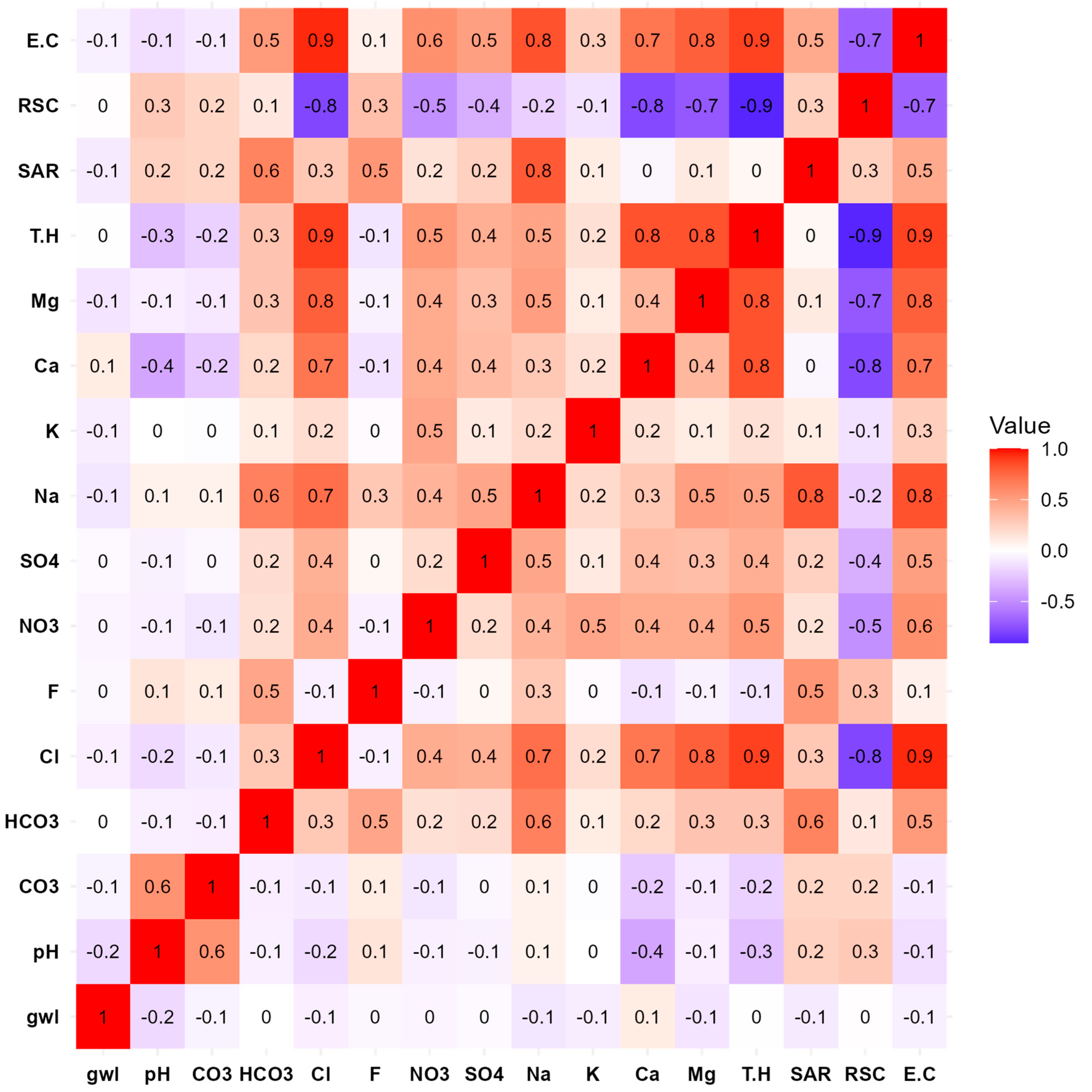
Furthermore, Figure 3 depicts the physical characteristics of the variables involved in the current study, informing of the time series plot and correlation heatmap as shown in Figure 4 respectively.

2.3. Artificial Neural Network (ANN)

The feed-forward neural network (FFNN) is the most often used neural network and the simplest kind of artificial network technique in the literature. The FFNN is sometimes known as a multilayer perceptron (MLP) or just a neural network. When the data are not sequential or time-dependent, the FFNN is commonly used [26]. The interaction between the input and output sets of nonlinear datasets is the focus of a regression model known as the FFNN. The ANN uses neurons to mimic the nervous system of the biological brain. With back-propagation (BP) computation, feed-forward neural networks (FFNNs) are frequently used to handle a variety of design issues [27]. The three levels that make up the FFNN structure are the input, hidden and output layers. The input layer has a fixed number of neurons or the number of features [28] in the dataset. After the input layer receives information about the inputs, it sends that information to the second layer. The hidden layer, which sits between the input and output layers, uses several neurons to apply the transformation from the input layer to the output layer. The strength of the connections between two neurons is reflected in the weight of each neuron in the hidden layer. The goal or aspect of the issue that we are attempting to predict is the output layer [29,30,31,32,33].

2.4. Generalized Regression Neural Network (GRNN)

In 1991, Dr. Donald Specht invented the general regression neural network, a type of probabilistic neural network. This neural network does not require iteration and just needs a portion of the training data. The use of a probabilistic neural network is quite beneficial since it can connect to the underlying function of the data just with a little training dataset [34]. The GRNN is comparable to a kernel regression network-based form of the radial basis neural network (RBFNN) structure [35,36]. Figure 2 shows its four layers, which are as follows: the input layer, which has the same dimension as the input vector, the pattern layer, which has the same number of neurons as the learning sample, the summation layer, which consists of two different types of neurons for summing, and the output layer (where the dimension k of the output vector in the learning sample is equal to the number of neurons in the output layer) [36,37].

2.5. EVNN Model

The evidential neural network for regression (EVNN) is a specialized neural network renowned for its adeptness in generating predictive probabilities and evaluating uncertainty. This model utilizes distance-based methods in regression, where the quantification of prediction uncertainty is achieved through a belief function applied to the real number line. The distances between input vectors and prototypes are considered as evidence, depicted as Gaussian random fuzzy numbers (GRFNs) and combined using the generalized product intersection rule [38]. The EVNN combines neural network architecture with regression techniques to capture complex nonlinear patterns in the data [39,40,41].
A GFN, a fuzzy subset of R with a membership function, as defined in Equation (1):
φ x ; m , h = e x p h 2 x m 2
where m R represents the mode, and h 0 , + indicates precision.
The vectors w 1 , , w K , representing K vectors in the p-dimensional feature space, are known as prototypes. Equation (2) measures the similarity between an input vector x and prototype w k :
s k x = e x p γ k 2 x w k 2  
Here, γ k is a positive scaling parameter. The evidence of prototype w k is portrayed as a GRFN in Equation (3):
Y ~ k x N ~ μ k x , σ k 2 , s k x h k
For training the EVNN model, the regularized average loss detailed in Equation (4) can be utilized:
C λ , e , ξ , ρ R Ψ = C λ , ϵ Ψ + ξ K k = 1 K h k + ρ K k = 1 K γ k 2
Here, ξ and ρ serve as regularization coefficients.
Five hyperparameters emerge from the EVNN model: the count K of prototypes, coefficients ϵ and λ , along with regularization coefficients ξ and ρ , as specified in Equation (4) (EVNNLoss).

2.6. Robust Linear Regression (RLR)

When the data contain outliers or violate the ordinary least squares (OLS) principles, robust linear regression, an extension of OLS regression, tries to produce more accurate estimations of the regression coefficients [42]. It is intended to perform well even in the presence of outliers and be less sensitive to extreme findings. The fundamental principle of robust linear regression (RLR) is to reduce the importance of outliers or significant observations when estimating the parameters. Instead of the squared residuals used in OLS, a new loss function called a robust loss function is often employed to achieve this [43]. The Huber loss, which combines the squared loss for small residuals with the absolute loss for large residuals, is one often employed for robust loss function. The Huber loss strikes a balance between the squared loss’s effectiveness and robustness. Iteratively reweighting the observations depending on their residuals and estimating the regression coefficients using weighted least squares are both steps in the estimation process for robust linear regression. In order to lessen the impact of outliers, the weights are set based on the robust loss function [44].

2.7. Model Validation and Evaluation Metrics

Model validation is a crucial step in ensuring that a model is reliable and performs well on unseen data. It helps prevent overfitting and provides an estimate of how the model will generalize to new datasets [45,46]. The current study employs the use of K-Fold Cross-Validation, in which the dataset is divided into k equally sized “folds”. The model is trained on k − 1 folds and tested on the remaining one. This process is repeated k times, with a different fold used for testing each time. The performance metrics are averaged across the fold to provide an overall estimate. Other validation techniques include the train–test split, bootstrap validation, time series validation, etc.
Various evaluation metrics are used to assess the performance of a model. These metrics measure aspects such as accuracy, error, uncertainty and how well the model generalizes to unseen data. In this research, five statistical measures were employed to assess the precision of the models: mean square error (MSE), root mean square error (RMSE), Pearson correlation coefficient (PCC) and coefficient of determinacy (R2). The performance criteria’s formal ranges are presented in Table 1, which are commonly utilized in studies to gauge the anticipated model’s performance.

2.8. Sensitivity Test

This kind of test is used to determine how different input variables impact the output of a model. It helps identify which inputs are the most influential, how much uncertainty in the inputs affects the results and whether the model is robust to changes in input values. It can be used in different ways to determine which input variables have the most significant impact on the model’s output [46]. Also, it can be used to understand how uncertainty in inputs propagates through the model to affect predictions. Moreover, there are different types of sensitivity test, such as one-at-a-time (oat) analysis, global sensitivity analysis, local sensitivity analysis, etc. [46]. The current study utilizes the one-at-a-time (oat) analysis method, which consists of varying one input parameter at a time while keeping all others constant over a specified range. It is considered to be simple and computationally inexpensive.

3. Results and Discussion

Exploratory and Dependency

Table 2 and Figure 4 serve as the background for the development of the cutting-edge evidential–neurocomputing approach for modeling groundwater salinization. The variation between the input variables and the targets indicates the impact of physicochemical parameters on groundwater salinization, which is significant in calibrating reliable and satisfactory models. Furthermore, Figure 4 gives an important insight to the properties of the groundwater as well as its physicochemical variables towards understanding the salinization process. Also, Figure 4 depicts the correlation analysis of the variables, which demonstrates both the direction and degree of the linear relationship of two quantified variables using the heatmap Pearson’s correlation coefficient. Each cell in the heatmap is colored according to the magnitude of the value it represents. Darker or more saturated colors typically indicate higher values, while lighter colors represent lower values. The distribution ranges between −1 and +1, whereby −1 represents a completely negative relationship, +1 indicates a perfect positive relationship and 0 denotes no relationship between two quantified variables. Therefore, examining the correlation matrix analysis demonstrates that there is a strong positive correlation between the target (EC) and Cl, Na, T.H and Mg. Also, NO3, SO4, Ca and SAR illustrate a moderate positive correlation with EC. RSC demonstrates a moderate negative connection with the target. Furthermore, F and K showed a weak positive relation with the target variable, while a weak negative correlation was demonstrated by groundwater level (gwl), pH and CO3 with the target variable inform of EC.
Furthermore, sensitivity analysis, which is considered a technique used to determine how different values of an input variable can impact a particular output variable under a given set of assumptions, is a crucial tool used to assess the robustness and reliability of models and predictions. Therefore, Table 2 demonstrates the results of sensitivity analysis carried out using the Gaussian process regression (GPR) method, whereby the first modeling schema group (G1) is composed of the following variables: gwl, pH, CO3, HCO3, Cl, F, NO3, SO4, Na, K, Ca, Mg, T.H, SAR and RSC. Furthermore, the second modeling schema group (G2) consists of Cl, T.H, SO4, Na, Ca, Mg and RSC. The third modeling schema group (G3), which input variables for the estimation of the groundwater salinization based on EC values, comprises gwl, pH, CO3, HCO3, F, NO3, K and SAR. Hence, this grouping of the input variables was carried out based on the sensitivity analysis demonstrated in Table 2.
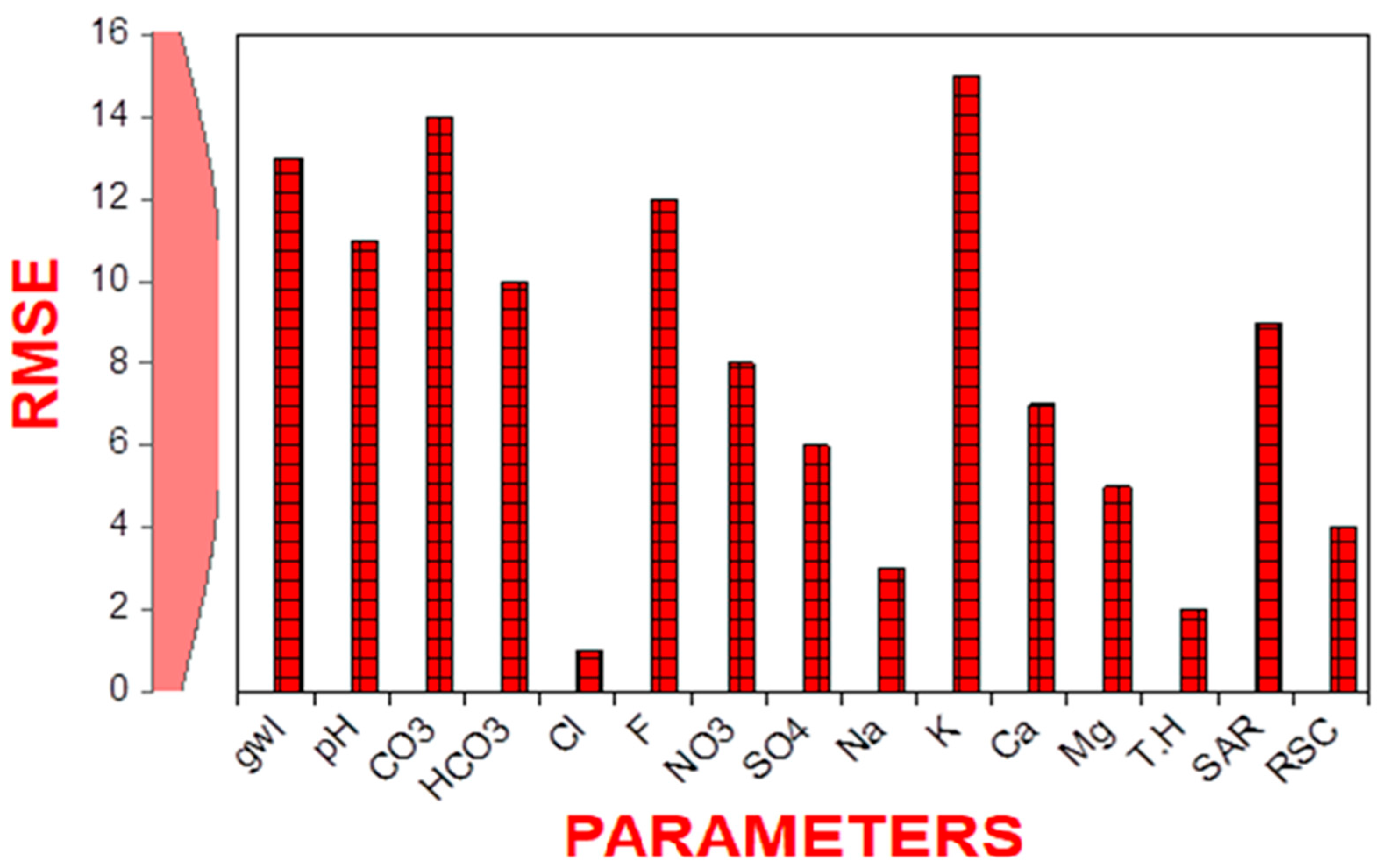
Furthermore, Figure 5 presents the graphical illustration of the sensitivity analysis based on their respective RMSE values. The lower the RMSE values, the better the performance of a certain variable and vice versa.
Furthermore, the current work involved the application of three different neurocomputing techniques, EVNN, ANN and GRNN, together with the classical RLR linear approach for the estimation of groundwater salinization. As mentioned earlier, the variables were grouped into three categories (G1, G2 and G3) based on the sensitivity analysis, which is used in modeling EC as the target using the neurocomputing techniques, as demonstrated in Table 3.
Table 3 presents the performance of the neurocomputing techniques (EVNN, ANN and GRNN) using four objective functions (R2, PC, MSE and RMSE) in three categories (G1, G2 and G3).
The obtained quantitative results demonstrated in Table 3 illustrate that the G2 input grouping depicts a more substantial performance than G1 and G3 for groundwater salinization estimation using neurocomputing techniques (EVNN, ANN and GRNN). Nevertheless, for the RLR classical model G1 depicts the highest performance accuracy in both the calibration and validation phases. Overall, the EVNN as a cutting-edge neurocomputing technique demonstrates the highest performance accuracy in both the calibration and validation phases, respectively, and has the capability of boosting the performance of the RLR classical method up to 46% and 46.4% in both the calibration and validation stages, respectively.
The quantitative EVNN results obtained in the current study are outstanding compared to recent studies conducted in the literature, for instance Abba et al. [47] The modeling schema were based on the actual field and experimental data. The results indicated the potential of GRNN-C1, with a value of NSE = 0.998 and 0.928 in the calibration and validation phases, respectively. The outcomes revealed weaknesses in all other stand-alone models, with a low efficiency that ranged from 0 to 60%. The attained ensemble results proved promising for all, with ANFIS-E-C1 (RMSE = 2.993, MAE = 0.879 and NSE = 0.999) emerging as best in the validation phase, but still the result was less than our finding for EVNN-G1 (R2 = 1.000, PCC = 1.000, MSE = 8.469 × 10⁻¹¹ and RMSE = 8.64 × 10⁻⁶) in the testing phase. Also, Sahour et al. [48] attained the highest accuracy of R2 = 0.89 and NSE = 0.87, which is also lower than our simulated results. The difference in the predicted outcomes could be due to the nature and the type of input variables explored. Moreover, one of the major limitations of the current study is the use of only neural network-based models; hence, the performance at a certain level can be enhanced using various state-of-the-art metaheuristic algorithms such as BBO, HHO, etc.
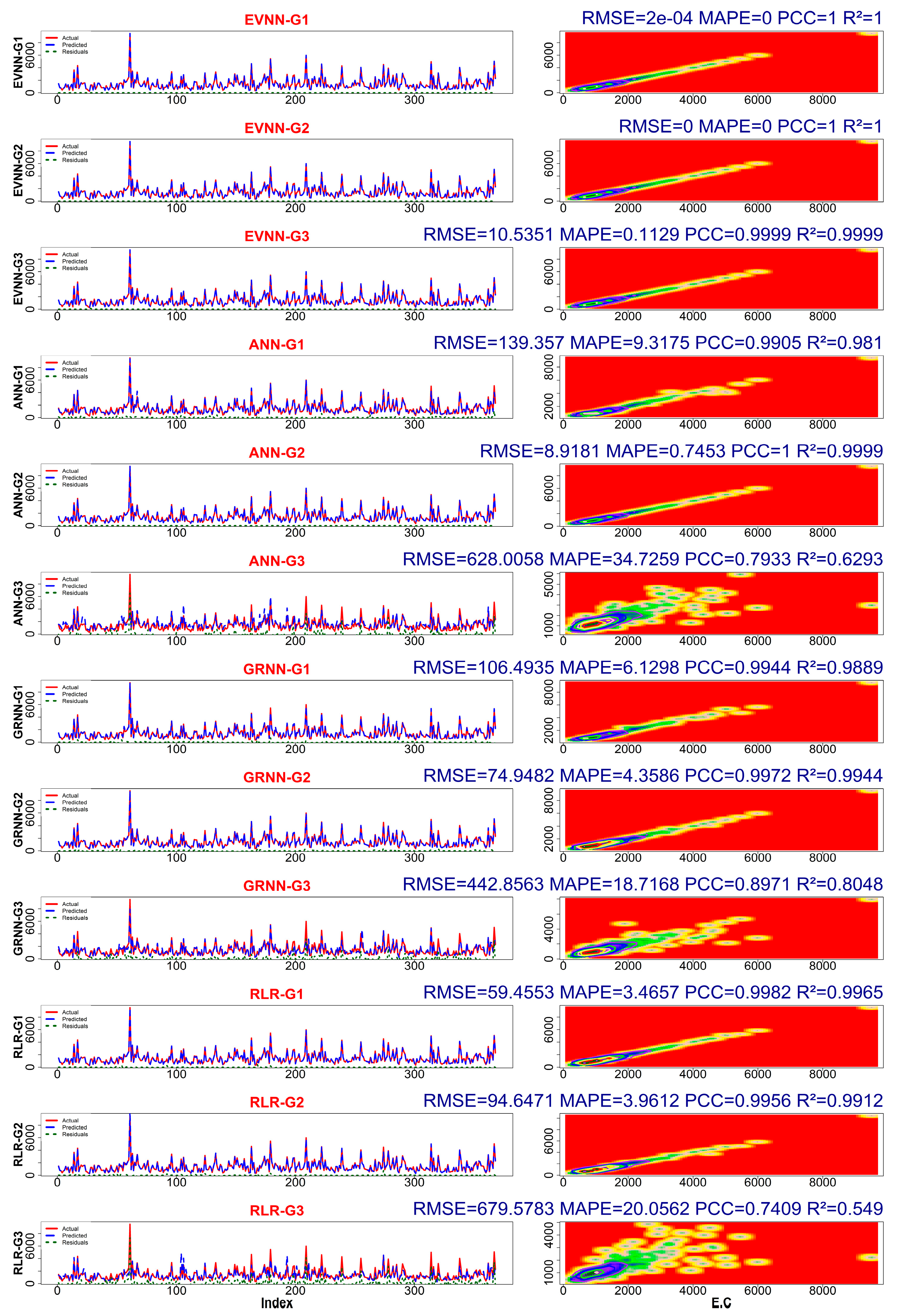
The predictive performance of the neurocomputing techniques combined with the classical RLR model can be visualized using a composite plot, which includes a time series plot (left) and a contour plot (right). Contour plots, which display data using color shading, help identify trends and changes across continuous variables, making complex 3D relationships easier to interpret. Figure 6 highlights performance metrics of models like EVNN-G1 and EVNN-G2, showing near-perfect accuracy (RMSE ≈ 0, PCC = 1, R² = 1). EVNN-G3, though slightly less accurate, still performs well, while ANN-G3, GRNN-G3 and RLR-G3 show a comparatively lower performance.
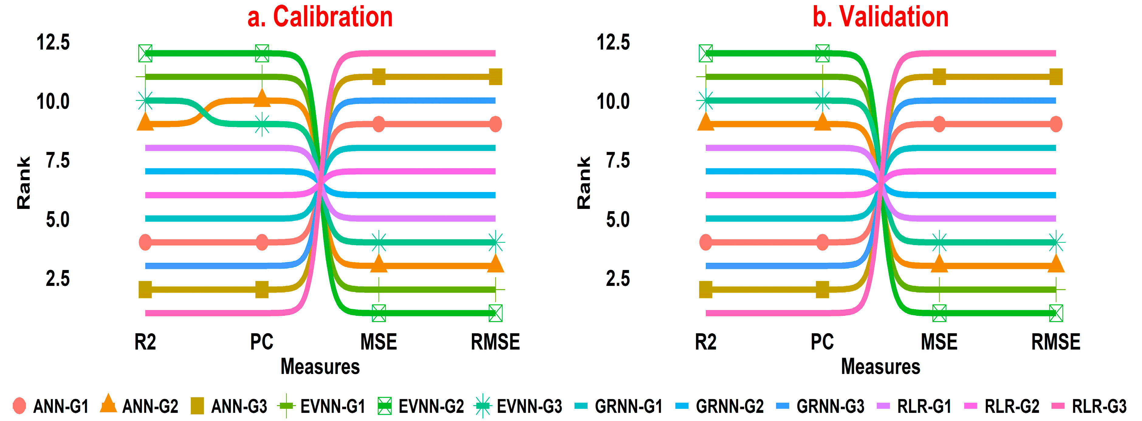
Furthermore, Figure 7 depicts the bump plot, which compares the performance of the techniques used in modeling the groundwater salinization based on four different objective functions (R2, PC, MSE and RMSE). A bump plot is a sort of visualization that can illustrate the ranking of various items over time or across multiple categories. It is particularly useful when comparing how the rank or position of an entity (such as individuals, teams or items) changes over different conditions. Rather than displaying raw values, a bump plot focuses on rank or order, showing how items move up or down relative to each other. Furthermore, each item is represented by a line that “bumps” up or down as its rank changes across the x-axis. Different items or groups are often color-coded to distinguish them easily and make it simpler to follow their movement over time. The visualization emphasizes changes in rank, making it easier to spot trends, outliers or significant shifts. These plots allow the comparison of many items at once as well as highlight the dynamics of the rankings rather than just static values. Moreover, the bump plot provided illustrates the ranking of various models (ANN-G1, ANN-G2, ANN-G3, EVNN-G1, EVNN-G2, EVNN-G3, GRNN-G1, GRNN-G2, GRNN-G3, RLR-G1, RLR-G2, RLR-G3) based on four distinct performance metrics: R2, PC, MSE and RMSE. The plot is divided into two phases: calibration and validation. EVNN-G1 and EVNN-G2 consistently rank first across all metrics in both phases, indicating that they are the most reliable and accurate algorithm combinations. Meanwhile, GRNN-G1, GRNN-G2, RLR-G1 and RLR-G2 perform moderately, often securing mid-range rankings across most metrics. In contrast, ANN-G3, GRNN-G3 and RLR-G3 rank lowest across all measures, reflecting their poor overall performance.
Additionally, another visualization chart namely, the Taylor plot, as shown in Figure 8, can be used in the graphical comparison of the techniques. A Taylor plot is a graphical representation of the relationship between three statistical measures: the model’s correlation coefficient, standard deviation and root mean squared error (RMSE). It is used to evaluate the performance of several models in comparison to one another and observable data. Therefore, Figure 8 compares the cutting-edge techniques’ performance based on their correlation coefficient and standard deviation values. The radial distance from the origin represents the standard deviation of the model’s predictions. Models closer to the reference standard deviation line (green arc) perform better. The angular position indicates the correlation coefficient between model predictions and observations. A stronger correlation (closer to one) suggests an improved performance. Also, the concentric circles centered on the reference point show varying amounts of RMSE. The smaller the RMSE values, the better the performance of the techniques. This Taylor plot clearly shows that EVNN models are the most accurate and dependable, whereas ANN-G3, GRNN-G3 and RLR-G3 are the least effective based on the performance measures provided.

4. Conclusions

Monitoring groundwater salinization is critical since it has major implications for environmental sustainability, agriculture, public health and economic stability. Increased salinity levels can harm the aquatic environment, reducing the richness of lakes, rivers and wetlands. Also, salinization can cause soil structure degradation, lowering its ability to support vegetation and increasing erosion risks. Additionally, high salt levels in groundwater can cause health issues such as hypertension and other cardiovascular illnesses. Therefore, accurate data on groundwater salinization assist policymakers in developing policies and plans for water management and agriculture. The current study utilizes various neurocomputing approaches (EVNN, ANN and GRNN) together with the classical linear approach (RLR) in modeling groundwater salinization. Before dwelling upon the modeling schema, the correlation and sensitivity analysis of the inputs and output was conducted to understand the behavior of the inputs towards the output. Hence, the summary of the findings of the current study can be summarized as follows:
i.
The correlation matrix analysis demonstrates that there is strong positive correlation between the target (EC) and Cl, Na, T.H and Mg. Also, NO3, SO4, Ca and SAR illustrate a moderate positive correlation with EC. RSC demonstrates a moderate negative connection with the target. Furthermore, F and K showed a weak positive relation with the target variable, while a weak negative correlation was demonstrated by gwl, pH and CO3 with the target variable.
ii.
Three different modeling schema groups in the form of G1 (gwl, pH, CO3, HCO3, Cl, F, NO3, SO4, Na, K, Ca, Mg, T.H, SAR and RSC), G2 (Cl, T.H, SO4, Na, Ca, Mg and RSC) and G3 (gwl, pH, CO3, HCO3, F, NO3, K and SAR) were arrived at based on the sensitivity analysis results.
iii.
The obtained quantitative results illustrate that the G2 input grouping depicts a substantial performance compared to G1 and G3 for groundwater salinization estimation using neurocomputing techniques (EVNN, ANN and GRNN).
iv.
Nevertheless, for the RLR classical model G1 depicts the highest performance accuracy in both the calibration and validation phases.
v.
Both EVNN-G1 and EVNN-G2 present excellent performance metrics (RMSE ≈ 0, MAPE = 0, PCC = 1, R2 = 1), indicating a perfect prediction accuracy, while EVNN-G3 demonstrates a slightly lower performance than EVNN-G1 and EVNN-G2, but is still highly accurate (RMSE = 10.5351, MAPE = 0.1129, PCC = 0.9999, R2 = 0.9999).
vi.
Overall, EVNN as a cutting-edge neurocomputing technique demonstrates the highest performance accuracy in both the calibration and validation phases, respectively, and has the capability of boosting the performance as against the RLR classical method up to 46% and 46.4% in both the calibration and validation stages, respectively.
vii.
Lastly, the quantitative predictive performance of the neurocomputing techniques together with the classical RLR were demonstrated using various state-of-the-art visualizations, including a contour plot embedded with a response plot, a bump plot and a Taylor diagram.
viii.
Finally, the current study equally indicated that the performance obtained from the neurocomputing techniques can be enhanced using various state-of-the-art metaheuristic algorithms such as BBO, HHO, etc.

Author Contributions

Conceptualization, A.G.U., S.M. and M.M.J.; Data curation, S.M., S.R.N., M.M.J., J.U. and S.M.H.S.; Formal analysis, A.G.U.; Investigation, A.G.U., M.M.J., J.U., S.M.H.S. and S.I.A.; Methodology, A.G.U., S.M., J.U. and S.I.A.; Resources, S.M.; Supervision, S.R.N.; Validation, M.M.J., S.I.A. and S.R.N.; Writing—original draft, S.M., S.R.N., M.M.J., J.U., S.M.H.S. and S.I.A. All authors have read and agreed to the published version of the manuscript.

Funding

This research received no external funding.

Data Availability Statement

The data presented in this study are available on request from the corresponding author. The data are not publicly available due to privacy or ethical restrictions.

Conflicts of Interest

The authors declare no conflicts of interest.

References

  1. Mirzavand, M.; Ghasemieh, H.; Sadatinejad, S.J.; Bagheri, R. An overview on source, mechanism and investigation approaches in groundwater salinization studies. Int. J. Environ. Sci. Technol. 2020, 17, 2463–2476. [Google Scholar] [CrossRef]
  2. Salama, R.B.; Otto, C.J.; Fitzpatrick, R.W. Contributions of groundwater conditions to soil and water salinization. Hydrogeol. J. 1999, 7, 46–64. [Google Scholar] [CrossRef]
  3. Faye, S.; Maloszewski, P.; Stichler, W.; Trimborn, P.; Faye, S.C.; Gaye, C.B. Groundwater salinization in the Saloum (Senegal) delta aquifer: Minor elements and isotopic indicators. Sci. Total Environ. 2005, 343, 243–259. [Google Scholar] [CrossRef]
  4. Yassin, M.A.; Usman, A.G.; Abba, S.I.; Uzun, D.; Aljundi, I.H. Intelligent learning algorithms integrated with feature engineering for sustainable groundwater salinization modelling: Eastern Province of Saudi Arabia. Results Eng. 2023, 20, 101434. [Google Scholar] [CrossRef]
  5. Essink, G.H.P.O. Improving fresh groundwater supply F problems and solutions. Ocean Coast. Manag. 2018, 44, 429–449. [Google Scholar] [CrossRef]
  6. Bennetts, D.A.; Webb, J.A.; Stone, D.J.M.; Hill, D.M. Understanding the salinisation process for groundwater in an area of south-eastern Australia, using hydrochemical and isotopic evidence. J. Hydrol. 2006, 323, 178–192. [Google Scholar] [CrossRef]
  7. Jakeman, A.J.; Barreteau, O.; Hunt, R.J.; Rinaudo, J.-D.; Ross, A. Integrated Groundwater Management; Springer: Cham, Switzerland, 2016. [Google Scholar]
  8. Bouksila, F.; Bahri, A.; Berndtsson, R.; Persson, M.; Rozema, J.; Van Der Zee, S.E.A.T.M. Assessment of soil salinization risks under irrigation with brackish water in semiarid Tunisia. Environ. Exp. Bot. 2010, 92, 176–185. [Google Scholar] [CrossRef]
  9. Wu, J.; Li, P.; Qian, H. Assessment of soil salinization based on a low-cost method and its influencing factors in a semi-arid agricultural area, northwest China. Environ. Earth Sci. 2014, 71, 3465–3475. [Google Scholar] [CrossRef]
  10. Besser, H.; Mokadem, N.; Redhouania, B.; Rhimi, N. GIS-based evaluation of groundwater quality and estimation of soil salinization and land degradation risks in an arid Mediterranean site (SW Tunisia). Arab. J. Geosci. 2017, 10, 350. [Google Scholar] [CrossRef]
  11. Gkiougkis, I.; Kallioras, A.; Pliakas, F.; Pechtelidis, A.; Diamantis, V.; Diamantis, I.; Ziogas, A.; Dafnis, I. Assessment of soil salinization at the eastern Nestos River Delta, N.E. Greece Catena Assessment of soil salinization at the eastern Nestos River Delta. CATENA 2015, 128, 238–251. [Google Scholar] [CrossRef]
  12. Schoups, G.; Hopmans, J.W.; Young, C.A.; Vrugt, J.A.; Wallender, W.W.; Tanji, K.K.; Panday, S. Sustainability of irrigated agriculture in the San Joaquin Valley, California. Proc. Natl. Acad. Sci. USA 2005, 102, 15352–15356. [Google Scholar] [CrossRef] [PubMed]
  13. Brunner, P.; Kinzelbach, W.; Li, W.P.; Dong, X.G. Sustainable irrigation in the Yanqi basin, China. WIT Trans. Ecol. Environ. 2006, 96, 115–125. [Google Scholar] [CrossRef]
  14. Yakirevich, A.; Weisbrod, N.; Kuznetsov, M.; Villarreyes, C.A.R.; Benavent, I.; Chavez, A.M.; Ferrando, D. Modeling the impact of solute recycling on groundwater salinization under irrigated lands: A study of the Alto Piura aquifer, Peru. J. Hydrol. 2013, 482, 25–39. [Google Scholar] [CrossRef]
  15. Han, D. Hydrochemical and isotopic evidences for deciphering conceptual model of groundwater salinization processes in a coastal plain, north China. Hydrol. Earth Syst. Sci. Discuss. 2017. [Google Scholar] [CrossRef]
  16. Motevalli, A.; Pourghasemi, H.R.; Hashemi, H.; Gholami, V. 25—Assessing the Vulnerability of Groundwater to Salinization Using GIS-Based Data-Mining Techniques in a Coastal Aquifer. In Spatial Modeling in GIS and R for Earth and Environmental Sciences; Elsevier, Inc.: Amsterdam, The Netherlands, 2019. [Google Scholar] [CrossRef]
  17. Nair, I.S.; Brindha, K.; Elango, L. Assessing the origin and processes controlling groundwater salinization in coastal aquifers through integrated hydrochemical, isotopic and hydrogeochemical modelling techniques. Hydrol. Sci. J. 2021, 66, 152–164. [Google Scholar] [CrossRef]
  18. Le Vo, P.; Tran, D.A.; Pham, T.L.; Le Thi Thu, H.; Viet, N.N. Advances in Research on Water Resources and Environmental Systems; Springer: Cham, Switzerland, 2022. [Google Scholar] [CrossRef]
  19. Zaresefat, M. Revolutionizing Groundwater Management with Hybrid AI Models: A Practical Review. Water 2023, 15, 1750. [Google Scholar] [CrossRef]
  20. Bayatzadeh Fard, Z.; Ghadimi, F.; Fattahi, H. Use of artificial intelligence techniques to predict distribution of heavy metals in groundwater of Lakan lead-zinc mine in Iran. J. Min. Environ. 2017, 8, 35–48. [Google Scholar] [CrossRef]
  21. Zare, M.; Koch, M. Title: Department of Geohydraulics and Engineering Hydrology, University of Kassel. J. Hydro-Environment Res. 2017, 18, 63–76. [Google Scholar] [CrossRef]
  22. Chen, W.; Li, Y.; Tsangaratos, P.; Shahabi, H.; Ilia, I. Applied sciences Groundwater Spring Potential Mapping Using Artificial Intelligence Approach Based on Kernel Logistic Regression, Random Forest, and Alternating Decision Tree Models. Appl. Sci. 2020, 10, 425. [Google Scholar] [CrossRef]
  23. Band, S.S.; Janizadeh, S.; Pal, S.C.; Chowdhuri, I.; Siabi, Z.; Norouzi, A.; Melesse, A.M.; Shokri, M.; Mosavi, A. Comparative Analysis of Artificial Intelligence Models for Accurate Estimation of Groundwater. Sensors 2020, 20, 5763. [Google Scholar] [CrossRef]
  24. Nosair, A.M.; Shams, M.Y.; AbouElmagd, L.M.; Hassanein, A.E.; Fryar, A.E.; Abu Salem, H.S. Predictive model for progressive salinization in a coastal aquifer using artificial intelligence and hydrogeochemical techniques: A case study of the Nile Delta aquifer, Egypt. Environ. Sci. Pollut. Res. 2022, 29, 9318–9340. [Google Scholar] [CrossRef] [PubMed]
  25. Barmpalexis, P.; Karagianni, A.; Karasavvaides, G.; Kachrimanis, K. Comparison of multi-linear regression, particle swarm optimization artificial neural networks and genetic programming in the development of mini-tablets. Int. J. Pharm. 2018, 551, 166–176. [Google Scholar] [CrossRef] [PubMed]
  26. Mahmoud, I.A.; Muhammad, U.J.; Kawu, S.J.; Magaji, M.M.; Jibril, M.M. Machine Learning-Based Wind Speed Estimation for Renewable Energy Optimization in Urban Environments: A Case Study in Kano State, Nigeria. Adv. J. Sci. Technol. Eng. 2024, 4, 35–51. [Google Scholar] [CrossRef]
  27. Jibril, M.M.; Malami, S.I.; Muhammad, U.J.; Bashir, A.; Usman, A.G.; Salami, B.A.; Rotimi, A.; Ibrahim, A.G.; Abba, S.I. High strength concrete compressive strength prediction using an evolutionary computational intelligence algorithm. Asian J. Civ. Eng. 2023, 24, 3727–3741. [Google Scholar] [CrossRef]
  28. Jibril, M.M.; Zayyan, M.A.; Malami, S.I.; Usman, A.G.; Salami, B.A.; Rotimi, A.; Abba, S.I. Applications in Engineering Science Implementation of nonlinear computing models and classical regression for predicting compressive strength of high-performance concrete. Appl. Eng. Sci. 2023, 15, 100133. [Google Scholar] [CrossRef]
  29. Haruna, S.I.; Malami, S.I.; Adamu, M.; Usman, A.G.; Farouk, A.I.; Ali, S.I.A.; Abba, S.I. Compressive Strength of Self-Compacting Concrete Modified with Rice Husk Ash and Calcium Carbide Waste Modeling: A Feasibility of Emerging Emotional Intelligent Model (EANN) Versus Traditional FFNN. Arab. J. Sci. Eng. 2021, 46, 11207–11222. [Google Scholar] [CrossRef]
  30. Usman, J.; Salami, B.A.; Gbadamosi, A.; Adamu, H.; Usman, A.G.; Benaafi, M.; Abba, S.I.; Othman, M.H.D.; Aljundi, I.H. Intelligent optimization for modelling superhydrophobic ceramic membrane oil flux and oil-water separation efficiency: Evidence from wastewater treatment and experimental laboratory. Chemosphere 2023, 331, 138726. [Google Scholar] [CrossRef]
  31. Malami, S.I.; Musa, A.A.; Haruna, S.I.; Aliyu, U.U.; Usman, A.G.; Abdurrahman, M.I.; Bashir, A.; Abba, S.I. Implementation of soft-computing models for prediction of flexural strength of pervious concrete hybridized with rice husk ash and calcium carbide waste. Model. Earth Syst. Environ. 2021, 8, 1933–1947. [Google Scholar] [CrossRef]
  32. Usman, A.G.; Ahmad, M.H.; Danraka, N.; Abba, S.I. The effect of ethanolic leaves extract of Hymenodictyon floribundun on inflammatory biomarkers: A data-driven approach. Bull. Natl. Res. Cent. 2021, 45, 128. [Google Scholar] [CrossRef]
  33. Uzun Ozsahin, D.U.; Precious Onakpojeruo, E.P.; Bartholomew Duwa, B.; Usman, A.G.; Isah Abba, S.I.; Uzun, B. COVID-19 Prediction Using Black-Box Based Pearson Correlation Approach. Diagnostics 2023, 13, 1264. [Google Scholar] [CrossRef]
  34. Panda, B.N.; Bahubalendruni, M.V.A.R.; Biswal, B.B. A general regression neural network approach for the evaluation of compressive strength of FDM prototypes. Neural Comput. Appl. 2015, 26, 1129–1136. [Google Scholar] [CrossRef]
  35. Wang, S.F.; Tang, Y.; Li, X.B.; Du, K. Analyses and predictions of rock cuttabilities under different confining stresses and rock properties based on rock indentation tests by conical pick. Trans. Nonferrous Met. Soc. China 2021, 31, 1766–1783. [Google Scholar] [CrossRef]
  36. Yang, A.M.; Zhuansun, Y.X. Prediction of compressive strength based on visualization of pellet microstructure data. J. Iron Steel Res. Int. 2021, 28, 651–660. [Google Scholar] [CrossRef]
  37. Alam, M.S.; Gazder, U. Shear strength prediction of FRP reinforced concrete members using generalized regression neural network. Neural Comput. Appl. 2020, 32, 6151–6158. [Google Scholar] [CrossRef]
  38. Den, T. An Evidential Neural Network Model for regression based on random fuzzy numbers. In International Conference on Belief Functions; Springer International Publishing: Cham, Switzerland, 2022. [Google Scholar]
  39. Denœux, T. Quantifying Prediction Uncertainty in Regression Using Random Fuzzy Sets: The ENNreg Model. IEEE Trans. Fuzzy Syst. 2023, 31, 3690–3699. [Google Scholar] [CrossRef]
  40. Denœux, T. Reasoning with fuzzy and uncertain evidence using epistemic random fuzzy sets: General framework and practical models. Fuzzy Sets Syst. 2023, 453, 1–36. [Google Scholar] [CrossRef]
  41. Mati, S.; Radulescu, M.; Saqib, N.; Samour, A.; Ismael, G.Y.; Aliyu, N. Incorporating Russo-Ukrainian war in Brent crude oil price forecasting: A comparative analysis of ARIMA, TARMA and ENNReg models. Heliyon 2023, 9, e21439. [Google Scholar] [CrossRef]
  42. Varin, S. Comparing the Predictive Performance of Ols and 7 Robust Linear Regression Estimators on a Real and Simulated Datasets. Int. J. Eng. Appl. Sci. Technol. 2021, 5, 9–23. [Google Scholar] [CrossRef]
  43. Jibril, M.M.; Malami, S.I.; Jibrin, H.B.; Muhammad, U.J.; Duhu, M.A.; Usman, A.G.; Ibrahim, A.G.; Ozsahin, D.U.; Lawal, Z.K.; Abba, S.I. New random intelligent chemometric techniques for sustainable geopolymer concrete: Low-energy and carbon-footprint initiatives. Asian J. Civ. Eng. 2023, 25, 2287–2305. [Google Scholar] [CrossRef]
  44. Yu, C.; Yao, W. Robust Linear Regression: A Review and Comparison. Commun. Stat.-Simul. Comput. 2017, 46, 6261–6282. [Google Scholar] [CrossRef]
  45. Kiiza, C.; Pan, S.Q.; Bockelmann-Evans, B.; Babatunde, A. Predicting pollutant removal in constructed wetlands using artificial neural networks (ANNs). Water Sci. Eng. 2020, 13, 14–23. [Google Scholar] [CrossRef]
  46. Abba, S.I.; Benaafi, M.; Usman, A.G.; Aljundi, I.H. Sandstone groundwater salinization modelling using physicochemical variables in Southern Saudi Arabia: Application of novel data intelligent algorithms. Ain Shams Eng. J. 2023, 14, 101894. [Google Scholar] [CrossRef]
  47. Abba, S.I.; Benaafi, M.; Usman, A.G.; Aljundi, I.H. Inverse groundwater salinization modeling in a sandstone’s aquifer using stand-alone models with an improved non-linear ensemble machine learning technique. J. King Saud Univ. Comput. Inf. Sci. 2022, 34, 8162–8175. [Google Scholar] [CrossRef]
  48. Sahour, H.; Gholami, V.; Vazifedan, M. A comparative analysis of statistical and machine learning techniques for mapping the spatial distribution of groundwater salinity in a coastal aquifer. J. Hydrol. 2020, 591, 125–321. [Google Scholar] [CrossRef]
Figure 1. Study location with the spatial–temporal resolution of the wells.
Water 16 02873 g001
Figure 2. Overall flow chart of the methodology proposed.
Water 16 02873 g002
Figure 3. Data properties of the variables based on the time series plot.
Water 16 02873 g003
Figure 4. Target–input parameters relationship using a heatmap.
Water 16 02873 g004
Figure 5. Sensitivity analysis graphical performance based on their RMSE ranking.
Water 16 02873 g005
Figure 6. Comparison plots using a time series plot embedded with a contour plot.
Water 16 02873 g006
Figure 7. Comparison based on bump plots.
Water 16 02873 g007
Figure 8. Taylor plot for modeling groundwater salinization.
Water 16 02873 g008
Table 1. Performance evaluation.
NameFormulaRange
PCCPCC= i = 1 N ( Y o b s Y ¯ o b s ) ( Y c o m Y ¯ c o m ) i = 1 N ( Y o b s Y ¯ o b s ) 2 i = 1 N ( Y c o m Y ¯ c o m ) 2 (−1 < PCC < 1)
R2 R 2 = 1 j = 1 N ( Y ) o b s , j ( Y ) c o m , j 2 j = 1 N ( Y ) o b s , j ( Y ) ¯ o b s , j 2 (0 < R2 < 1)
MSE M S E = 1 N   i = 1 N ( Y o b s i Y c o m i ) 2 (0 < MSE < ∞)
RMSE R M S E = i = 1 N ( Y o b s i Y c o m i ) 2 N (0 < RMSE < ∞)
Note: N, Y o b s i , Y ¯ and Y c o m i are the data number, observed data, average value of the observed data and computed values, respectively.
Table 2. Sensitivity analysis results.
ParametersRMSERanking
gwl989.0413
pH953.0611
CO31010.4814
HCO3822.8310
Cl336.361
F978.9112
NO3763.088
SO4622.976
Na514.333
K6933.0015
Ca730.857
Mg614.095
T.H483.942
SAR814.669
RSC571.454
Table 3. Neurocomputing results for modeling groundwater salinization.
Calibration
R2PCMSERMSE
EVNN-G11.0001.0005.851 × 10−80.000242
EVNN-G21.0001.0007.463 × 10−118.64 × 10⁻⁶
EVNN-G31.0001.000152.40112.345
ANN-G10.9810.99026,666.788163.300
ANN-G20.9991.000109.20910.450
ANN-G30.6050.778541,552.264735.902
GRNN-G10.9890.99415,572.542124.790
GRNN-G20.9940.9977713.22187.825
GRNN-G30.8040.896269,301.500518.943
RLR-G10.9960.9984853.93169.670
RLR-G20.9910.99612,300.639110.908
RLR-G30.5380.733634,149.997796.335
Validation
EVNN-G11.0001.0006.811 × 10−80.000419
EVNN-G21.0001.0008.469 × 10−118.64 × 10⁻⁶
EVNN-G31.0001.000178.40115.080
ANN-G10.9790.98827,766.788189.300
ANN-G20.9970.998119.20913.450
ANN-G30.6030.776546,115.264798.902
GRNN-G10.9870.99220,135.542187.790
GRNN-G20.9920.99512,276.221150.825
GRNN-G30.8020.894273,864.500581.943
RLR-G10.9940.9969416.931132.670
RLR-G20.9890.99416,863.639173.908
RLR-G30.5360.731638,712.997859.335
Note: Bold for best-performing model.
Disclaimer/Publisher’s Note: The statements, opinions and data contained in all publications are solely those of the individual author(s) and contributor(s) and not of MDPI and/or the editor(s). MDPI and/or the editor(s) disclaim responsibility for any injury to people or property resulting from any ideas, methods, instructions or products referred to in the content.