Abstract
The reliable observation and accurate estimates of land–atmosphere water vapor (H2O) flux is essential for ecosystem management and the development of Earth system models. Currently, the most direct measurement method for H2O flux is eddy covariance (EC), which depends on the development of fast-response H2O sensors. In this study, we presented a cost-efficient open-path H2O analyzer (model: HT1800) based on the tunable diode laser absorption spectroscopy (TDLAS) technique, and investigated its applicability for measuring atmospheric turbulent flux of H2O using the EC method. We prepared two HT1800 analyzers with lasers that operate at wavelengths of 1392 nm and 1877 nm, respectively. The field performance of the two analyzers was evaluated through inter-comparative experiments with LI-7500RS and IRGASON, two of the most commonly used H2O analyzers in the EC community. Water vapor densities measured by the three types of analyzers had high overall agreement with the reference sensor; however, they all experienced drift. The mean density drifts of HT1800, LI-7500 and IRGASON were 3.7–5.2%, 4.0% and 3.8%, respectively. Even so, the half-hourly H2O fluxes measured by HT1800 were highly consistent with those by LI-7500RS and IRGASON (with a difference of less than 2%), suggesting that HT1800 can obtain H2O fluxes with high confidence. The HT1800 was also proved to be suitable for EC application in terms of data availability, flux detection limit and response to the high-frequency turbulent variation. Furthermore, we investigated how the spectroscopic effect influences the measurements of H2O density and flux. Despite the fact that the 1392 nm laser was much more susceptible to the spectroscopic effect, the fluxes after correcting for this bias showed excellent agreement with the IRGASON fluxes. Considering the cost advantage in laser and photodetector, the HT1800 analyzer using a 1392 nm infrared laser is a promising and economical solution for EC measurement studies of water vapor.
1. Introduction
Water vapor is the most important greenhouse gas in the atmosphere and plays a significant role in the Earth’s water and energy balance [1]. Water vapor flux describes the net exchange rate of water vapor between land surface and atmosphere. It can also be expressed as latent heat flux, representing the amount of energy required to evaporate a unit of water per time. From the hydrological perspective, the concept of evapotranspiration (ET) is widely used, which refers to the combined loss of water due to evaporation from the soil surface and transpiration from the plant through stomata [2]. The accurate and reliable observation data of water vapor and ET flux is critical for the development of Earth system models and ecosystem management like drought monitoring and irrigation planning [3,4].
The eddy covariance (EC) technique is recognized as the standard method for measuring the turbulent fluxes of energy, carbon and water vapor across a wide range of ecosystem types [5]. It is already in widespread use, particularly in global and regional ecosystem networks (e.g., FLUXNET). To apply the EC technique, instantaneous fluctuations of wind velocity and water vapor (or other gas species) concentration must be simultaneously measured at sufficient frequency (≥10 Hz). Usually, the latter is obtained using a fast-response and high-precision analyzer. Most flux sites currently use non-dispersive infrared absorption gas analyzers (hereafter referred to as NDIR analyzers) that are already commercially available, e.g., LI-7500 produced by LI-COR Biosciences (Lincoln, NE, USA) and EC150 produced by Campbell Scientific Inc. (CSI) (Logan, UT, USA). These NDIR analyzers typically include a broadband infrared light source, a detector and band-pass filters to select a wavelength range that spans absorption lines for water vapor and carbon dioxide (CO2), enabling the simultaneous detection of both gases [6,7,8]. Regarding the sensor structure, the NDIRs can be divided into two categories: open-path and closed-path. Open-path sensors are used far more frequently than closed-path sensors because they need less manual maintenance, have less high-frequency attenuation and require simpler data-processing steps [9,10].
In addition to instrumental performance, the cost of the gas analyzer is also a practical aspect for users to consider. If one is only interested in ET, an analyzer that just measures water vapor is a viable option, as long as its performance is comparable with the abovementioned NDIRs, while also having a clear advantage in cost. For this reason, we have developed a cost-efficient open-path water vapor analyzer (model HT1800, HealthyPhoton Technology Co., Ltd., Ningbo, China), which applies the technology of tunable diode laser absorption spectroscopy (TDLAS). Unlike NDIR, TDLAS uses a narrow linewidth laser source in the near- or mid-infrared band, changes the wavelength by tuning the laser current and temperature and scans the absorption spectral line of a specific molecule. These characteristics make it possible to monitor atmospheric gas species with great sensitivity and very short response times, which is necessary for a successful EC measurement. Furthermore, the most crucial parts of a TDLAS analyzer, the laser and the photodetector, can utilize the mature fabrication processes widely used in the optical communication industry, for example, the vertical cavity surface emitting laser (VCSEL). The current cost of the HT1800 analyzer is at least one third of the existing commercial NDIRs. Based on the historical price of other VCSEL lasers used for fiber communication [11], we can expect a lower instrument price once it is ready for mass production.
Several TDLAS-based water vapor sensors and their applications have been reported in the past [12,13,14,15]. Most of them had employed lasers with wavelengths between 1.3 μm and 2.7 μm. However, the majority of these sensors were used for concentration monitoring, while just a few were designed for EC flux measurements [16,17,18], and of these, only one study had performed a long-term (25 d) flux study to test the performance of their TDLAS sensor [18]. This sensor measured similar water vapor flux dynamic to that of LI-7500, but there was a noticeable difference in the flux magnitude on some specific days. The general idea of HT1800, such as operating principle and light path design, is similar to the above TDLAS analyzer, but we have different motivations and questions to be addressed in this study. First, HT1800 is defined as a mass-produced instrument for the EC community. With its compact size, low power consumption and consistent performance, the HT1800 is expected to meet the demand for EC flux measurements. Second, recent studies have emphasized the importance of spectroscopic effect correction for EC flux calculation while using a laser-based gas analyzer [19]. This additional correction raises from the absorption line broadening due to atmospheric water vapor, temperature and pressure fluctuations [20]. However, when using different laser wavelengths, the correction can vary by orders of magnitude [21]. Therefore, choosing a proper laser source is quite necessary to minimize flux uncertainty associated with this correction term. However, this issue has not been discussed in the studies mentioned above.
In this study, we prepared two HT1800 analyzers, equipped with an infrared laser near 1392 nm and 1877 nm, respectively. The 1877 nm band has the advantage that no other absorbing atmospheric gas is present, and its absorption rate is comparable to that of the 1392 nm band [22,23]. The 1392 nm laser is one of the most popular options for the TDLAS detection of water vapor, since lasers and photodetectors that operate at this wavelength are easily available and relatively inexpensive [14], but its broadening effect is much stronger than the 1877 nm line according to the HITRAN database [24]. Using the two HT1800 analyzers, we carried out two EC experiment campaigns at an agricultural site in eastern China. Two widely used commercial NDIR analyzers, LI-7500RS (LI-COR Biosciences, Lincoln, NE, USA) and EC150 (Campbell Scientific Inc., Logan, UT, USA), were employed for side-by-side comparison with HT1800. The purposes of this study are (1) to test the performance of HT1800 under field conditions and evaluate its applicability for measuring turbulent water vapor fluxes, and (2) quantify and compare the spectroscopic effect on the water vapor fluxes of two HT1800 analyzers with different infrared laser wavelengths. Meanwhile, we proposed a hypothesis that the 1392 nm analyzer can yield reliable water vapor fluxes after accounting for the spectroscopic correction.
2. Materials and Methods
2.1. Instrument Design
The HT1800 analyzer employs a low-power VCSEL and an Indium Galinide Arsenide (InGaAs) photodetector (model G12182-110K, Hamamatsu Photonics, Hamamatsu, Shizuoka, Japan). It uses the TDLAS technique, which modifies the wavelength by changing the driving current and temperature of the VCSEL to scan the absorption spectrum of H2O (hereinafter H2O refers to water vapor unless otherwise stated). We applied the wavelength modulation spectroscopy (WMS) technique to modulate the VCSEL’s driving current at a high frequency (fm). The modulation shifts the absorption information to harmonics of fm, which leads to an improved signal-to-noise ratio [25].
Figure 1 shows the design of the HT1800 analyzer. The open-path configuration has the laser beam collimated and sent to a flat reflective mirror 0.25 m away from the VCSEL. Three rigid posts support the mirror to form a single reflection with an effective optical path length of 0.5 m. An InGaAs photodetector detects the reflected laser beam and transforms the optical intensity into an electrical signal for further processing. Temperature of the laser and the detector is stabilized by Peltier thermoelectrical coolers (TEC). The VCSEL, InGaAs photodetector, TEC control and laser driving electronics are all integrated in an airtight aluminum sensor housing (sensor head) with two optical windows for emitting and receiving collimated laser beams. A water-proof control box encloses a printed circuit board (PCB) with a field programmable gate array (FPGA) and microcontroller units (MCUs). The PCB realizes the analog/digital signal generation, modulation, sampling, processing and system-controlling electronics. The whole analyzer operates between −20 and 50 °C with a typical power consumption of 10 W at the steady state. The sensor head has a weight of 2.5 kg, with dimensions of 450 mm (length) and 90 mm (diameter). The size of the control box is 340 × 300 × 150 mm3, and the weight is approximately 1.5 kg. The sensor head and control box are connected by a driving/signal cable no longer than 3 m.
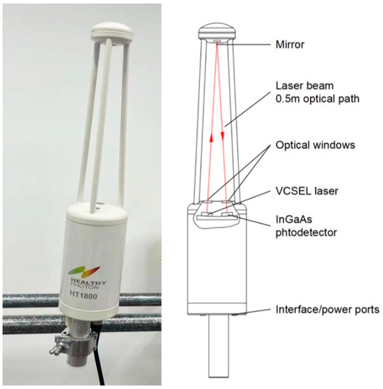
Figure 1.
A photograph and the technical design of the HT1800 open-path water vapor analyzer.
2.2. Signal Processing and Concentration Retrieval
The analyzer adopts the WMS technique that modulates the laser driving current with a 20 kHz sinusoidal waveform. It scans across the selected pressure-broadened absorption line of H2O by a 100 Hz ramp waveform. The signal output from the InGaAs photodetector passes through an analog-to-digital converter (ADC). After that, an FPGA-based two-channel lock-in amplifier demodulates the first (1f) and the second (2f) harmonics of the sinusoidal signal simultaneously. The 1f signal is a dimensionless number proportional to the laser intensity received by the detector, so we define it as optical signal strength (OSS), which indicates the cleanliness of the windows and mirrors along the laser path. At each ramp scan, the 2f signal is normalized by the 1f signal. The normalized spectrum (2f/1f) is projected onto a reference spectrum stored in the instrument to generate a signal proportional to the H2O density [26].
The reference spectrum is acquired during calibration process using several gas samples with known H2O concentrations at stable temperature and pressure conditions. Coefficients generated from the multiple concentrations are applied to calculate the raw molecular density of H2O, which is stored at 10 Hz frequency for EC flux calculation.
2.3. Calibration
The HT1800 analyzer was calibrated using a multi-point calibration scheme, which included H2O densities of 0, 9, 19 and 28 g m−3. The zero gas was from a high-pressure tank with pure nitrogen, and gas samples of the other three calibration points were provided by a commercially available dew point generator (DPG) (model LI-610, LI-COR Biosciences, Lincoln, NE, USA) at a room temperature of 30 °C. The calibration gas was delivered into a Teflon calibration tube that enclosed the open optical path of HT1800 at a flow rate of 1000 cm3 min−1. Once the instrument yields a stable concentration, the signal output from the photodetector is extracted to acquire the first and the second order harmonics. The normalized second harmonic signal (2f/1f) is stored as the reference spectrum associated with each calibration density. A second-order polynomial was used to fit the normalized signal strengths against the calibration points, and a correlation coefficient of 0.99 was obtained throughout the entire calibration range. The calibration accuracy is constrained by the gas mixtures generated by the DPG that has a dew point accuracy of ±0.2 °C, which is equivalent to ±0.7% to ±1.9% of H2O density.
2.4. Analysis of Instrumental Noise
The Allan variance was calculated [27] using a sample of 10 Hz data acquired in the laboratory, to estimate the instrumental noise (i.e., measurement precision) of the HT1800 analyzer. The analyzer was placed inside an enclosed environment chamber (model HWS-250B, Tianjin Taisite Instrument, Tianjin, China) with a temperature setting of 25 °C. Similar to the operation steps of calibration, a gas sample with mole fraction of near 104 μmol mol−1 (ppmv) continuously passed through the optical path that was sealed with a Teflon tube. After the readings stabilized, 30-min data were collected for the calculation of the Allan variance. The instrumental noise was determined as the root square of the Allan variance. The reason for choosing a 104 ppmv gas sample was to compare with the noise level of the two commercial NDIR analyzers.
2.5. Eddy Covariance Measurements
Eddy covariance measurements of H2O fluxes were conducted at an agricultural site using HT1800 and two commercial open-path analyzers that are widely used in the EC community. The site was located in the National Agricultural Experiment Station for Soil Quality (31°27′09.205″ N, 120°25′33.222″ E, 4 m a.s.l.) of the Suzhou Academy of Agricultural Sciences of China. The measurements were carried out during two periods in 2022, from 7 May to 16 May (hereinafter referred to as P-1) and from 10 September to 5 October (hereinafter referred to as P-2). During P-1, field plots in the experimental area were cultivated with wheat with a canopy height of 0.7 m (Figure 2a). During P-2, the fields were covered by rice plants and the canopy height was on average 0.85 m (Figure 2b). According to footprint analysis [28], more than 85% of the flux sources were from the wheat and rice fields.
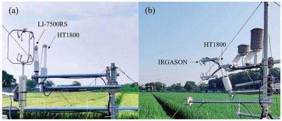
Figure 2.
Pictures of the experimental fields and the eddy covariance instruments during the measurement periods of (a) 7–16 May 2022 and (b) 10 September–5 October 2022.
Eddy covariance instruments and the setup information are shown in Figure 2 and Table 1. The HT1800 analyzers deployed during P-1 and P-2 were equipped with an infrared laser operating near 1877 nm and 1392 nm, respectively. Two sonic anemometers from different manufacturers were used during the two periods, and the wind data were shared by two H2O analyzers for calculating the eddy fluxes. During P-2, we used an EC150 open-path analyzer and a CSAT-3 anemometer, which were integrated into a flux system named IRGASON by the manufacturer (Campbell Scientific, Inc., Logan, UT, USA). Therefore, we will now refer to EC150 as IRGASON. All instruments were powered by a solar panel and battery system. All three open-path analyzers were calibrated before the two inter-comparative experiments. A CR6 data logger (Campbell Scientific, Inc., Logan, UT, USA) was used to store the 10 Hz raw data from the LI-COR system (P-1) and IRGASON system (P-2). Data from HT1800 was saved in another CR6, and its clock was synchronized to the other one from time to time. In addition, a low-drift temperature and humidity probe (model HMP155, Vaisala, Helsinki, Finland) was available to record half-hourly H2O densities, which was used as a benchmark to evaluate the measurement drifts of the three H2O analyzers.

Table 1.
Information of the eddy covariance instruments for water vapor (H2O) flux measurements during P-1 (7–16 May 2022) and P-2 (10 September–5 October 2022).
2.6. Processing of Eddy Covariance Data
2.6.1. Flux Calculation
The EddyPro software (version 7.0.9, LI-COR Biosciences, Lincoln, NE, USA) was used to calculate the sensible heat flux (H), water vapor flux (Fv) and latent heat flux (LE) following the standard procedure recommended by CarboEurope-IP [29].
Here, w is the vertical wind velocity; ρa and ρv are the densities of dry air and H2O, respectively; Ta is the air temperature; cp is the specific heat capacity of dry air; λ is the latent heat of vaporization for water; the prime symbol represents the instantaneous deviation from the means; the overbar represents the mean of the instantaneous products (i.e., covariance of the two quantities) over the flux averaging period (30 min).
2.6.2. Flux Correction
The H2O fluxes were corrected for three aspects. The first is caused by the flux losses in the high- and low-frequency ranges of the spectrum. The second correction arises from the temperature and H2O fluctuations, which is well known as the WPL correction [30]. The third, which we call spectroscopic correction, is to account for the changes in the absorption line shape of H2O due to temperature, pressure and humidity fluctuations in the environment [20]. Here, line shape changes due to humidity fluctuation are called self-broadening.
The spectral losses were compensated using the commonly accepted analytical solutions [31,32]. The WPL and spectroscopic effects can be jointly corrected, according to Equation (4) [19].
In Equation (4), Fv is the corrected H2O flux; ρraw is the H2O density directly measured by HT1800; ρv is the corrected H2O density considering the spectroscopic effect; μ is the molar mass ratio of dry air to H2O; represents the sensible heat flux. It is worth mentioning that Equation (4) requires the accurate H2O density ρv. Here, the half-hourly mean H2O density can be experimentally determined using the HITRAN database [24], simulations of the TDLAS system [21], and the simultaneously measured temperature and pressure from slow-response sensors. A, B, and C are dimensionless parameters, which are derived in a similar way. Since the turbulent H2O density cannot be corrected to due to the lack of 10-Hz temperature and pressure measurements in the optical path of HT1800, we can rearrange Equations (2) and (4) to Equation (5) in order to solve the corrected H2O flux Fv.
2.6.3. Quality Control of Water Vapor Fluxes
Water vapor fluxes were quality controlled following several criteria. First, flux data were rejected if the gas analyzer had low values of OSS (varying between 0 and 100); a threshold of 70 was accepted for LI-7500RS and IRGASON according to the manufacturer’s suggestion, and 40 was used for HT1800 based on the laboratory test [33]. Second, quality flags were assigned to each half-hourly flux after stationarity and integral turbulence characteristic tests [34], and those with a flag of “2” were rejected as bad data. Third, any fluxes exceeding three times the standard deviation in a window of one day were eliminated as spikes. To acquire more half-hourly flux data for inter-comparison, we did not apply the friction velocity filtration on the nighttime fluxes.
2.6.4. Spectral Analysis
For each half-hourly period, power spectra and cospectra of the most relevant variables (air temperature and water vapor) were calculated using fast Fourier transform method according to the commonly accepted procedures [35]. The purpose is to examine whether the spectra and cospectra shapes agree with those expected under ideal turbulent conditions [36], and to evaluate HT1800’s performance in capturing the eddies responsible for the turbulent flux, particularly in the higher frequencies. The calculated spectra and cospectra were binned into a number of logarithmically spaced classes, for which the mean values were calculated. Then, normalized forms of power spectra (Sx(f)) of the variable x and cospectra (Cowx(f)) between w and x were calculated, where they were multiplied by the sampling frequency (f) and divided by their variance (var(x)) and covariance (cov(w, x)), respectively. The normalized spectra and cospectra were plotted against the normalized frequency (nm) according to nm = f(z − d)/U, where z is the measurement height, d is the displacement height (0.7 times the canopy height) and U is the wind speed.
3. Results and Discussion
3.1. Instrumental Noise and Flux Detection Limit
Instrumental noise is an important indicator of a gas analyzer’s performance because it characterizes the measurement precision and, subsequently, the flux detection limit. Figure 3 displays the H2O mole fraction measured by two HT1800 analyzers at 10 Hz over a 30 min period, together with the corresponding Allan variance as a function of integration time. High-frequency fluctuations dominated both H2O time series. In the 1392 nm data, more data points varied from the mean concentration (near 104 ppmv), implying that larger measurement noise was detected. The Allan variance patterns of the two HT1800 were similar, which decreased with a slope of near −1 up to an integration time of 60–80 s. It means that white noise, or high-frequency signal fluctuation, dominated this domain. At a larger integration time, the Allan variance began to level off or increase due to low-frequency drift produced by external noise. The root square of the Allan variance can be regarded as the instrumental noise or measurement precision. In this instance, the noise levels of the 1877 nm and 1392 nm HT1800 analyzers were 9.5 and 12.4 ppmv, respectively, at the integration time of 0.1 s (i.e., 10 Hz sampling frequency).
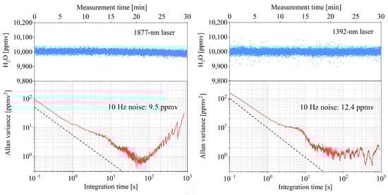
Figure 3.
Water vapor (H2O) mole fraction (blue dots) measured at 10 Hz over a 30 min period by two HT1800 analyzers, together with the corresponding Allan variance (red lines) as a function of integration time. Panels on the left correspond to the analyzer with a 1877 nm laser, while those on the right are the analyzer with a 1392 nm laser. The downwards dashed lines with a slope of −1 represent the theoretical behavior of white noise.
We compared the instrumental noises produced by HT1800, LI-7500RS and IRGASON. The 1877 nm and 1392 nm HT1800 analyzers were estimated with a 10-Hz noise of 9.5 and 12.4 ppmv, respectively. This is a factor of 2.0–2.6 larger than that of LI-7500RS (4.7 ppmv) according to LI-COR specification, which is derived by testing 104 ppmv H2O under similar conditions to this study. The HT1800 is also nearly twice the noise level of IRGASON, which is roughly estimated based on the information provided by CSI. Apparently, LI-7500RS and IRGASON show superiority in this respect, although their estimates might not be so optimistic under all environmental conditions. Nevertheless, the instrumental noise of H2O receives less attention due to its high atmospheric abundance and relatively small noise error. In this study, for example, the HT1800 noise is only approximately 0.1% of the measured H2O concentration. Using the instrumental noise as mentioned above, we calculated the detection limits of the two HT1800 analyzers for measuring half-hourly fluxes [37]; the results are 0.08 and 0.11 g m−2 h−1 for the 1877 nm and 1392 nm HT1800, respectively, which are both less than 0.1 W m−2 if converted into the form of latent heat flux. With this detection limit, HT1800 can capture most ecosystem H2O fluxes, because in most environmental conditions the ET flux and dew deposition flux (i.e., negative H2O flux) have a substantially larger magnitude [38,39,40].
3.2. Weather Conditions during Field Experiments
During the first experimental period (P-1), the half-hourly air temperature (Ta) varied between 13.0 and 27.8 °C (mean: 19.4 °C) and a total of 12.8 mm precipitation occurred from the noon of 12 May to the morning of 13 May (Figure 4a). During the second experimental period (P-2), there was greater variation in the air temperature, which ranged from 12.7 to 36.1 °C (mean: 22.9 °C) (Figure 5a). The air temperature was fairly high from October 1 to 3, with a maximum Ta of 32.0–36.1 °C at noon, which was followed by a significant drop on 4 October. During P-2, there were also a number of rainy days that contributed to a cumulative precipitation of 135.1 mm. The diurnal variation pattern of Ta was notably weakened by the rainfall events (Figure 5a).
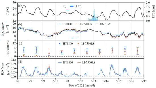
Figure 4.
(a) Half-hourly air temperature (Ta) and precipitation (PPT), (b) half-hourly water vapor (H2O) densities measured by HT1800, LI-7500RS and a low-drift temperature and humidity probe (HMP155, Vaisala), (c) daily mean drift of HT1800 and LI-7500RS for H2O density measurements and (d) half-hourly H2O fluxes measured by HT1800 and LI-7500RS from 7 to 16 May 2022. H2O drift in panel (c) is defined as the absolute density difference between HT1800 or LI-7500RS and HMP155, divided by the HMP155 density; the vertical bars represent the standard deviation derived from the half-hourly results.
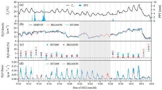
Figure 5.
(a) Half-hourly air temperature (Ta) and precipitation (PPT), (b) half-hourly water vapor (H2O) densities measured by HT1800, IRGASON and a low-drift temperature and humidity probe (HMP155, Vaisala), (c) daily mean drift of HT1800 and IRGASON for H2O density measurements and (d) half-hourly H2O fluxes measured by HT1800 and IRGASON from 10 September to 5 October 2022. H2O drift in panel c is defined as the absolute density difference between HT1800 or IRGASON and HMP155, divided by the HMP155 density; the vertical bars represent the standard deviation derived from the half-hourly results. The light grey shade indicates the period that came up with data logger malfunctions, leading to data gaps in the HMP155 densities from 21 to 27 September and the HT1800 densities from 26 to 27 September.
3.3. Water Vapor Density
The 10 Hz H2O densities measured by HT1800, LI-7500RS and IRGASON and the 1 Hz densities measured by HMP155 were averaged at a half-hourly basis for side-by-side comparison (Figure 4b and Figure 5b). Meanwhile, we used the HMP155 data as the reference to evaluate the measurement drift (or bias) of the three open-path analyzers, because HMP155 is widely recognized for its low-drift characteristic and reliability in field deployment. During P-1, the rejection rate of the half-hourly H2O density was 11.1% for HT1800 and 10.7% for LI-7500RS. During P-2, due to data logger malfunction, HT1800 data from 26–27 September and HMP155 data from 21–27 September were lost (Figure 5), and the data rejection rate was 15.8% for HT1800 and 12.3% for IRGASON. Laser signal degradation caused by rainfall had accounted for more than 90% of the rejected data.
During P-1, H2O densities measured by HT1800, LI-7500RS and HMP155 exhibited similar variation patterns, with mean values of 11.15, 11.15 and 11.40 g m−3, respectively (Figure 4b). LI-7500RS agreed with HMP155 much better than HT1800 for the first two days, which is also evidenced by the H2O drift in Figure 4c. Here, H2O drift is defined as the absolute density difference between HT1800 or LI-7500RS and HMP155, divided by the density of HMP155. From 10 to 12 May, the mean drift of HT1800 was 4.6% (systematically lower than HMP155), whereas the LI-7500RS was 3.9% (systematically higher than HMP155). Such pattern was reversed from 13 to 16 May, during which the HT1800 densities were 5.8% higher than HMP155 and LI-7500RS were lower by 4.3%. For the whole experimental period, the mean density drifts of HT1800 and LI-7500RS were 5.2% and 4.0%, respectively.
During P-2, we found good consistency between the HT1800 and IRGASON densities, with large variability ranging from 8.31 to 23.92 g m−3. The mean H2O densities from HT1800, IRGASON and HMP155 were 17.03, 16.92 and 17.23 g m−3, respectively (Figure 5b). Data from 22 to 27 September were not taken into account due to data gap caused by data logger malfunction. Figure 5c shows that HT1800 had a slightly smaller drift than IRGASON before the gap, whereas it reversed after the gap. There was a sharp fall of air temperature on 4–5 September, during which the H2O density dropped by nearly two-thirds, and both HT1800 and IRGASON observed lower densities with respect to HMP155. On the whole, the measurement drifts of HT1800 and IRGASON were not significantly different during P-2, and the mean drifts were 3.7% and 3.8%, respectively.
Measurement drift is common for laser instruments. Calibration is generally performed under controlled conditions, so the measurement accuracy is sensitive to the changing environment in field deployment, particularly the temperature [41]. For NDIRs, the temperature-induced drift is usually determined experimentally and compensated on the output signals according to the real-time temperature [7]. Such drift compensation was also considered in HT1800′s signal processing, but was performed by an algorithm for real-time identification of spectral line peak positions. However, drift is never completely avoidable. In this study, H2O densities measured by the three gas analyzers were in generally good agreement with the HMP155 reference, but temporal drift existed in different directions and magnitudes. The relationship between the measurement drift and the air temperature was shown in Figure 6. We can clearly see that the drift occurred in steps, rather than with a continuous pattern. The data points were visually distributed in separate groups (filled with three different colors), and most of them have a significant linear correlation (p < 0.01) with the air temperature. The three groups of data correspond to the drifts of the different stages, which were divided by the time of significant change in environmental conditions (e.g., rainfall event) or instrument maintenance. Intercept and slope of the linear regression varied at different stages of both P-1 and P-2. This suggests that factors other than temperature may also lead to measurement bias. For LI-7500RS, as well as HT1800, the effectiveness of scrubber chemicals in the sensor could be one potential cause. The instrumental performance of HT1800 and its drift response to a wider span of environmental conditions will be investigated in the future.
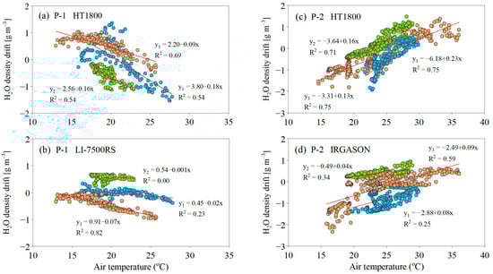
Figure 6.
Scatter plot of water vapor (H2O) density drift against air temperature during (a,b) P1 and (c,d) P2. The drift is calculated as the density deviation of each H2O analyzer (HT1800, LI-7500RS and IRGASON) from the reference sensor (HMP155). P-1 and P-2 refer to the measurement periods of 7–16 May 2022 and 10 September–5 October 2022, respectively. The blue, green and orange circles represent data from the three stages of each measurement period. The dates used to split the three stages are 9 May and 13 May for P-1, and 15 September and 27 September for P-2. Linear regression for each group of data were illustrated by the red line and the equation next to it.
3.4. Water Vapor Flux
The data availability of H2O fluxes measured by the three gas analyzers were close to each other. After applying quality control during P-1, 75.3% of the HT1800 fluxes and 73.3% of the LI-7500RS fluxes remained. During P-2, the availability of HT1800 and IRGASON fluxes were 79.8% and 84.0%, respectively. H2O fluxes measured by the three gas analyzers showed very strong visual agreement at the half-hourly basis (Figure 4d and Figure 5d). A more quantitative comparison is enabled by running linear regression analysis (Figure 7), which yields a slope of 0.998 between the HT1800 and LI-7500RS fluxes (R2 = 0.983) and a slope of 1.016 between the HT1800 and IRGASON fluxes (R2 = 0.986). During P-1, both HT1800 and LI-7500RS produced a mean flux of 0.0255 g m−2 s−1. During P-2, the mean fluxes measured by HT1800 and IRGASON were 0.0295 and 0.0290 g m−2 s−1, respectively. As expected, we observed a clear diurnal variation pattern in the H2O fluxes, which is consistent with that of the air temperature (Figure 4 and Figure 5).
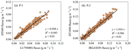
Figure 7.
Scatter plot of the half-hourly water vapor fluxes measured by (a) HT1800 and LI-7500RS during P-1 (7–16 May 2022), and (b) HT1800 and IRGASON during P-2 (10 September–October 2022). The solid lines show the linear regression with zero intercept.
Regardless of H2O density differences between the three analyzers, there was no significant effect on the H2O fluxes. For example, the HT1800 density drift was 3–6 times larger than that of LI-7500RS and IRGASON over the periods of 7–8 May and 29 September–1 October, but their flux differences were only 3–4%. This is because the calculation of EC fluxes is based on turbulent fluctuation, i.e., variation in H2O concentration on short time scale. Therefore, it is not a critical problem for flux measurement with the current level of density drift. In addition, the HT1800 density drift was associated with another uncertainty in the H2O flux, as the half-hourly mean density was involved in the calculation of WPL and spectroscopic correction ( in Equations (4) and (5)). We repeated this correction by using the density measured by HMP155 (representing the true density), resulting in a change of less than 1% in the HT1800 fluxes. Finally, considering the use of standard procedure for EC data processing and the high degree of consistency in the H2O fluxes, we believe that the flux data obtained from HT1800 can be used with confidence.
3.5. Effects of Flux Corrections on Water Vapor Fluxes of HT1800
Figure 8 shows the mean diurnal variations of different correction terms of the H2O fluxes measured by HT1800 and their respective ratio to the uncorrected flux. Correction for the spectral loss was firstly applied. It increased the H2O fluxes by on average 22.3% and 32.5% during P-1 and P-2, respectively. The magnitude of this correction was significantly greater in the daytime (Figure 8a,b), but its ratio to the uncorrected flux was slightly greater in the nighttime (Figure 8c,d). The spectral correction acted as the largest correction term during P-1.
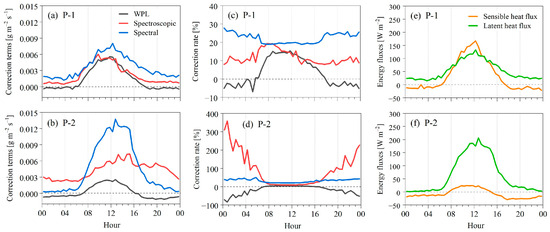
Figure 8.
Mean diurnal variations of (a,b) magnitudes of different correction terms of the water vapor flux, (c,d) correction rates of different correction terms and (e,f) sensible heat and latent heat fluxes during the experimental periods of 7–16 May (P-1) and 10 September–5 October (P-2) in 2022. WPL, spectroscopic and spectral in the legend refer to the correction terms due to WPL effect, spectroscopic effect and spectral loss in the high- and low-frequency ranges, respectively. Correction rate is defined as the ratio of the correction magnitude to the uncorrected flux.
The WPL correction term had a similar diurnal pattern to the spectral correction, but it could be negative. During P-1, the correction rate of WPL ranged from −6.9% to 15.4%, with higher values (positive) in the daytime. The correction rate showed a wider range during P-2, varying from −84.0% to 4.6%. The largest correction rate (negative) was observed at midnight, which was mainly due to the very weak nighttime evapotranspiration (Figure 8f). Given that the sensible heat (H) and latent heat (LE) fluxes are required to calculate the WPL term, the difference in the H and LE magnitudes between P-1 and P-2 (Figure 8e,f) could account for the majority of the difference in WPL correction rates between the two periods.
The correction term due to the spectroscopic effect had totally different regimes between the two periods. Despite having similar diurnal patterns, the mean magnitude of this term during P-2 was almost twice as great as it was during P-1 (Figure 8a,b). The correction rates between the two periods were considerably more different, being 11.8% and 93.9%, respectively. The correction rate during P-1 showed a very weak diurnal pattern (Figure 8c). On the other hand, during P-2, a strong diurnal pattern was seen, with surprisingly high correction rates (exceeding 300% of the uncorrected flux) at midnight and moderate correction rates (approximately 10%) at noon (Figure 8d).
To explain this, we investigated how the spectroscopic effect influence the measurements of H2O density and thus the flux. Figure 9 shows the spectroscopic correction factors for H2O density at different temperatures and pressures. We found that the 1392 nm absorption line is more susceptible to temperature change but less sensitive to pressure change. However, for the 1877 nm line, the pressure variation seems to cause much larger density bias. According to the temperature and pressure records during P-1 and P-2, both the H2O densities from the 1392 nm and the 1877 nm analyzers were subject to an overall negative bias (correction rates were less than 1). But the variation of the bias was far lower for the 1877 nm analyzer, because the ambient pressure changed very little at the experimental site. Similarly, the spectroscopic correction for H2O fluxes was also more temperature dependent for both 1392 nm and 1877 nm lasers, which is verified by the significant positive correlation between the correction magnitude and the temperature (p < 0.01). However, the 1392 nm laser-based measurement requires more correction than that of the 1877 nm, which explains the large flux correction rate during P-2 (Figure 8d). Especially at nighttime, when the temperature dropped significantly and the H2O fluxes were small, the flux correction can be as large as 300%. Even so, the corrected H2O fluxes are still regarded with high reliability due to their excellent consistency with the IRGASON fluxes (Figure 7b).
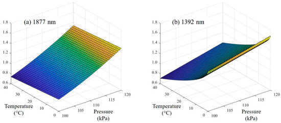
Figure 9.
Correction factors for water vapor density as a function of temperature and pressure for the (a) 1877 nm and (b) 1392 nm absorption lines due to changes in the line shape.
3.6. Spectral Characteristic
To examine the spectral characteristic of the three gas analyzers, we calculated the frequency-weighted, normalized power spectra and cospectra of H2O densities (Figure 10). Additionally presented are the power spectra and cospectra of the air temperature and the theoretical model [36]. Data in the figure are the ensemble averages of a selected period during P-1 (09:30–12:30 of 16 May 2022) and P-2 (09:00–13:00 of 29 September 2022), respectively. Weather conditions during the two periods were similar, with unstable stratification and wind speeds of 1.2–1.5 m s−1.
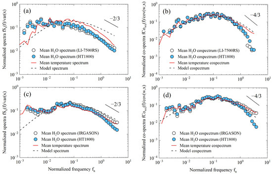
Figure 10.
Frequency-weighted, normalized spectra and cospectra of water vapor (H2O) and air temperature plotted against the normalized frequency. Data in the figure are the ensemble averages from 09:30 to 12:30 on 16 May 2022 (panels (a,b)) and from 09:00 to 13:00 on 29 September 2022 (panels (c,d)). The frequency is normalized to dimensionless form fn = f(z − d)/U, where f, z, d and U are the sampling frequency, measurement height, displacement height and wind speed, respectively. The spectra and cospectra are normalized by multiplying by the f and dividing by the respective variance (var(x)) and covariance (cov(w, x)). Black lines with slopes of −2/3 and −4/3 indicate the ideal behavior of spectra and cospectra in the inertial subrange, respectively, according to the theoretical model [36].
During the first selected period, the spectra of HT1800 and LI-7500RS were in good agreement but both deviated negatively from the Kaimal model spectrum (−2/3 slope) in the normalized frequency range of fn > 0.03 (Figure 10a). We also found deviation of the air temperature spectrum from the Kaimal model in the inertial subrange (fn > 0.2). The reason may attribute to the limited distance between the sensor height and the canopy top, because the Kaimal model may not apply there and the spectra shapes may be affected by atmospheric flow and specific turbulence formation [42]. The cospectra of both HT1800 and LI-7500RS were close to those of the model and the temperature cospecta at fn ≤ 0.5; but in higher frequencies, they began to deviate from the ideal slope (−4/3) in a similar way (Figure 10b). The overall high-frequency correction rates of the two analyzers during P-1 (21.1% and 21.0%, respectively) can also verify the similar attenuation of HT1800 and LI-7500RS cospectra in the high-frequency end. Therefore, we concluded that HT1800 and LI-7500RS had comparable capability in responding to the high-frequency turbulent variation.
During the second selected period, the spectra and cospectra of IRGASON matched up with the temperature and the model quite well, only with the exception in the frequency range of fn ≤ 0.01. Such spectral behavior in the low-frequency end was also observed during P-1, where we have discussed the potential cause. The spectra and cospectra of HT1800 displayed a pattern that was quite similar to IRGASON; however, this showed some attenuation at fn ≥ 1 (Figure 10c,d). As a result, IRGASON had clearly better spectral performance than HT1800. This is because IRGASON’s measurement paths of H2O and wind velocity were almost identical, so that high-frequency loss due to sensor separation was minimized.
4. Conclusions
This study presents a cost-efficient open-path water vapor (H2O) analyzer (model HT1800) based on the TDLAS technique, which is designed for measuring the atmospheric turbulent flux of H2O using the EC method. Considering the trade-off between optical device cost and magnitude of flux correction due to spectroscopic changes of the H2O absorption line, we presented two HT1800 analyzers with infrared lasers that operate at wavelengths of 1392 nm and 1877 nm, respectively. The field performance of the two HT1800 analyzers were evaluated through inter-comparative experiments with two NDIR-based sensors LI-7500RS and IRGASON, which are the most popular H2O analyzers in the EC community. The main conclusions are as follows.
- (1)
- H2O densities measured using the three types of gas analyzers were in generally good agreement with the reference sensor (HMP155), but temporal drift existed in different directions and magnitudes.
- (2)
- Despite density deviations, H2O fluxes measured by HT1800 were remarkably consistent with those measured by LI-7500RS and IRGASON. Therefore, we are confident that HT1800 can obtain accurate H2O fluxes both at half-hourly and daily timescale. Through the field experiments, HT1800 was also proved to be suitable for EC application in terms of data availability, flux detection limit and response to the high-frequency turbulent variation.
- (3)
- The spectroscopic effect can cause much larger measurement bias in the 1392 nm laser-based analyzer than the 1877 nm one, but the corrected H2O fluxes only differed by 2% from the reference instrument (IRGASON). Considering the cost advantage in laser and photodetector, the HT1800 analyzer using a 1392 nm laser is a promising and economical solution for EC measurement studies of water vapor.
In this study, the HT1800 was only evaluated in a few different environmental scenarios. In the future it is important to take additional experiments to improve the performance of this new analyzer also expand its applicability in a variety of environments.
Author Contributions
Conceptualization, K.W. and Y.W.; data curation, L.H., J.Z. and X.Z. (Xiaojie Zhen); formal analysis, L.H., J.Z. and T.-J.L.; investigation, L.H., J.Z., X.Z. (Xiaojie Zhen) and L.S.; methodology, K.W. and T.-J.L.; project administration, Y.W.; resources, L.S. and Y.W.; software, T.-J.L.; supervision, T.-J.L. and Y.W.; validation, X.Z. (Xunhua Zheng); visualization, K.W.; writing—original draft, K.W.; writing—review and editing, T.-J.L. and X.Z. (Xunhua Zheng). All authors have read and agreed to the published version of the manuscript.
Funding
This research was funded by the National Key R&D Program of China (grant number 2023YFC3705300), Hebei Provincial Department of Science and Technology of China (S&T Program of Hebei, grant number 22373903D), the National Natural Science Foundation of China (grant number 41975169) and Jiangsu Province Agricultural Science and Technology Independent Innovation Fund Project (grant number CX(22)3005).
Data Availability Statement
The data presented in this study are available from the corresponding author upon reasonable request. The data are not publicly available due to confidential agreements with instrument providers.
Acknowledgments
We thank Xiaohua Zhang from Jiangsu Tynoo Corporation for his technical support in field flux measurements.
Conflicts of Interest
Xiaojie Zhen was employed by Jiangsu Tynoo Corporation. Yin Wang was employed by HealthyPhoton Technology Co., Ltd. The remaining authors declare that the research was conducted in the absence of any commercial or financial relationships that could be construed as a potential conflict of interest.
References
- IPCC. 2021 Climate Change 2021: The Physical Science Basis; Masson-Delmotte, V., Zhai, P., Pirani, A., Connors, S.L., Péan, C., Berger, S., Caud, N., Chen, Y., Goldfarb, L., Gomis, M.I., et al., Eds.; Contribution of Working Group I to the Sixth Assessment Report of the Intergovernmental Panel on Climate Change; Cambridge University Press: Cambridge, UK; New York, NY, USA, 2021. [Google Scholar]
- Katul, G.G.; Oren, R.; Manzoni, S.; Higgins, C.; Parlange, M.B. Evapotranspiration: A Process Driving Mass Transport and Energy Exchange in the Soil-Plant-Atmosphere-Climate System. Rev. Geophy. 2012, 50, RG3002. [Google Scholar] [CrossRef]
- Allen, R.G.; Pereira, L.S.; Raes, D.; Smith, M. Crop Evapotranspiration: Guidelines for Computing Crop Water Requirements; FAO Irrigation and Drainage Paper 56; FAO: Rome, Italy, 1998. [Google Scholar]
- Wang, K.; Dickinson, R.E. A Review of Global Terrestrial Evapotranspiration: Observation, Modeling, Climatology, and Climatic Variability. Rev. Geophys. 2012, 50, 2011RG000373. [Google Scholar] [CrossRef]
- Baldocchi, D.; Falge, E.; Gu, L.; Olson, R.; Hollinger, D.; Running, S.; Anthoni, P.; Bernhofer, C.; Davis, K.; Evans, R.; et al. FLUXNET: A New Tool to Study the Temporal and Spatial Variability of Ecosystem-Scale Carbon Dioxide, Water Vapor, and Energy Flux Densities. Bull. Am. Meteorol. Soc. 2001, 82, 2415–2434. [Google Scholar] [CrossRef]
- Heikinheimo, M.J.; Thurtell, G.W.; Kidd, G.E. An Open Path, Fast Response IR Spectrometer for Simultaneous Detection of CO2 and Water Vapor Fluctuations. J. Atmos. Ocean. Technol. 1989, 6, 624–636. [Google Scholar] [CrossRef]
- Auble, D.L.; Meyers, T.P. An Open Path, Fast Response Infrared Absorption Gas Analyzer for H2O and CO2. Bound.-Layer Meteorol. 1992, 59, 243–256. [Google Scholar] [CrossRef]
- Billesbach, D.P.; Fischer, M.L.; Torn, M.S.; Berry, J.A. A Portable Eddy Covariance System for the Measurement of Ecosystem–Atmosphere Exchange of CO2, Water Vapor, and Energy. J. Atmos. Ocean. Technol. 2004, 21, 639–650. [Google Scholar] [CrossRef]
- Haslwanter, A.; Hammerle, A.; Wohlfahrt, G. Open-Path vs. Closed-Path Eddy Covariance Measurements of the Net Ecosystem Carbon Dioxide and Water Vapour Exchange: A Long-Term Perspective. Agric. For. Meteorol. 2009, 149, 291–302. [Google Scholar] [CrossRef]
- Polonik, P.; Chan, W.S.; Billesbach, D.P.; Burba, G.; Li, J.; Nottrott, A.; Bogoev, I.; Conrad, B.; Biraud, S.C. Comparison of Gas Analyzers for Eddy Covariance: Effects of Analyzer Type and Spectral Corrections on Fluxes. Agric. For. Meteorol. 2019, 272, 128–142. [Google Scholar] [CrossRef]
- Liu, A.; Wolf, P.; Lott, J.A.; Bimberg, D. Vertical-cavity surface-emitting lasers for data communication and sensing. Photon. Res. 2019, 7, 121–136. [Google Scholar] [CrossRef]
- May, R.D. Open-Path, Near-Infrared Tunable Diode Laser Spectrometer for Atmospheric Measurements of H2O. J. Geophys. Res. 1998, 103, 19161–19172. [Google Scholar] [CrossRef]
- Zondlo, M.A.; Paige, M.E.; Massick, S.M.; Silver, J.A. Vertical Cavity Laser Hygrometer for the National Science Foundation Gulfstream-V Aircraft. J. Geophys. Res. 2010, 115, D20309. [Google Scholar] [CrossRef]
- Novak, J.L.; Magryta, P.; Stacewicz, T.; Malinowski, S.P. Fast Optoelectronic Sensor of Water Concentration. Opt. Appl. 2016, 46, 607–618. [Google Scholar]
- Buchholz, B.; Afchine, A.; Klein, A.; Ebert, V.; Kramer, M.; Ebert, V. HAI, a New Airborne, Absolute, Twin Dual-Channel, Multi-Phase TDLAS-Hygrometer: Background, Design, Setup, and First Flight Data. Atmos. Meas. Tech. 2017, 10, 35–57. [Google Scholar] [CrossRef]
- Witt, F.; Nwaboh, J.; Bohlius, H.; Lampert, A.; Ebert, V. Towards a Fast, Open-Path Laser Hygrometer for Airborne Eddy Covariance Measurements. Appl. Sci. 2021, 11, 5189. [Google Scholar] [CrossRef]
- Li, M.; Kan, R.; He, Y.; Liu, J.; Xu, Z.; Chen, B.; Lu, Y.; Ruan, J.; Huang, X.; Deng, H.; et al. Development of a Laser Gas Analyzer for Fast CO2 and H2O Flux Measurements Utilizing Derivative Absorption Spectroscopy at a 100 Hz Data Rate. Sensors 2021, 21, 3392. [Google Scholar] [CrossRef] [PubMed]
- Gu, M.; Chen, J.; Mei, J.; Tan, T.; Wang, G.; Liu, K.; Liu, G.; Gao, X. Open-Path Anti-Pollution Multi-Pass Cell-Based TDLAS Sensor for the Online Measurement of Atmospheric H2O and CO2 Fluxes. Opt. Express 2022, 30, 43961. [Google Scholar] [CrossRef]
- Burba, G.; Anderson, T.; Komissarov, A. Accounting for Spectroscopic Effects in Laser-Based Open-Path Eddy Covariance Flux Measurements. Glob. Chang. Biol. 2019, 25, 2189–2202. [Google Scholar] [CrossRef]
- Burch, D.E.; Singleton, E.B.; Williams, D. Absorption Line Broadening in the Infrared. Appl. Opt. 1962, 1, 359–363. [Google Scholar] [CrossRef]
- Pan, D.; Benedict, K.B.; Golston, L.M.; Wang, R.; Collett, J.L.; Tao, L.; Sun, K.; Guo, X.; Ham, J.; Prenni, A.J.; et al. Ammonia Dry Deposition in an Alpine Ecosystem Traced to Agricultural Emission Hotpots. Environ. Sci. Technol. 2021, 55, 7776–7785. [Google Scholar] [CrossRef]
- Green, A.E.; Kohsiek, W. A Fast Response, Open Path, Infrared Hygrometer, Using a Semiconductor Source. Bound.-Layer Meteorol. 1995, 74, 353–370. [Google Scholar] [CrossRef]
- Le Barbu, T.; Vinogradov, I.; Durry, G.; Korablev, O.; Chassefière, E.; Bertaux, J.L. TDLAS a Laser Diode Sensor for the in Situ Monitoring of H2O, CO2 and Their Isotopes in the Martian Atmosphere. Adv. Space Res. 2006, 38, 718–725. [Google Scholar] [CrossRef]
- Rothman, L.S.; Barbe, A.; Chris Benner, D.; Brown, L.R.; Camy-Peyret, C.; Carleer, M.; Carleer, K.C.M.R.; Clerbaux, C.; Dana, V.; Devi, V.M.; et al. The HITRAN Molecular Spectroscopic Database: Edition of 2000 Including Updates through 2001. J. Quant. Spectrosc. Radiat. 2003, 82, 5–44. [Google Scholar] [CrossRef]
- Werle, P.; Slemr, F. Signal-To-Noise Ratio Analysis in Laser Absorption Spectrometers Using Optical Multipass Cells. Appl. Opt. 1991, 30, 430–434. [Google Scholar] [CrossRef] [PubMed]
- Dong, L.; Yu, Y.; Li, C.; So, S.; Tittel, F.K. Ppb-Level Formaldehyde Detection Using a CW Room-Temperature Interband Cascade Laser and a Miniature Dense Pattern Multipass Gas Cell. Opt. Express 2015, 23, 19821. [Google Scholar] [CrossRef]
- Werle, P.; Mücke, R.; Slemr, F. The Limits of Signal Averaging in Atmospheric Trace-Gas Monitoring by Tunable Diode-Laser Absorption Spectroscopy (TDLAS). Appl. Phys. B 1993, 57, 131–139. [Google Scholar] [CrossRef]
- Kljun, N.; Calanca, P.; Rotach, M.W.; Schmid, H.P. A Simple Two-Dimensional Parameterisation for Flux Footprint Prediction (FFP). Geosci. Model Dev. 2015, 8, 3695–3713. [Google Scholar] [CrossRef]
- Aubinet, M.; Grelle, A.; Ibrom, A.; Rannik, Ü.; Moncrieff, J.; Foken, T.; Kowalski, A.S.; Martin, P.H.; Berbigier, P.; Bernhofer, C.; et al. Estimates of the annual net carbon and water exchange of European forests: The EUROFLUX methodology. Adv. Ecol. Res. 2000, 30, 113–175. [Google Scholar]
- Webb, E.K.; Pearman, G.I.; Leuning, R. Correction of Flux Measurements for Density Effects due to Heat and Water Vapour Transfer. Q. J. R. Meteorol. Soc. 1980, 106, 85–100. [Google Scholar] [CrossRef]
- Moncrieff, J.B.; Massheder, J.M.; de Bruin, H.; Ebers, J.; Friborg, T.; Heusinkveld, B.; Kabat, P.; Scott, S.; Soegaard, H.; Verhoef, A. A System to Measure Surface Fluxes of Momentum, Sensible Heat, Water Vapor and Carbon Dioxide. J. Hydrol. 1997, 188–189, 589–611. [Google Scholar] [CrossRef]
- Moncrieff, J.B.; Clement, R.; Finnigan, J.; Meyers, T. Averaging, Detrending and Filtering of Eddy Covariance Time Series. In Handbook of Micrometeorology: A Guide for Surface Flux Measurements; Lee, X., Massman, W., Law, B., Eds.; Kluwer Academic Publishers: Dordrecht, The Netherlands, 2004; pp. 7–31. [Google Scholar]
- Wang, K.; Kang, P.; LU, Y.; Zheng, X.; Liu, M.; Lin, T.; Butterbach-Bahl, K.; Wang, Y. An Open-Path Ammonia Analyzer for Eddy Covariance Flux Measurement. Agric. For. Meteorol. 2021, 308–309, 108570. [Google Scholar] [CrossRef]
- Mauder, M.; Foken, T. Documentation and Instruction Manual of the Eddy-Covariance Software Package TK3 (Update); Arbeitsergebnisse; Universität Bayreuth, Abteilung Mikrometeorologie: Bayreuth, Germany, 2015. [Google Scholar]
- Stull, R.B. An Introduction to Boundary Layer Meteorology. In Atmospheric Science Library; Kluwer Academic Publishers: Dordrecht, The Netherlands, 2009; p. 666. [Google Scholar]
- Kaimal, J.C.; Wyngaard, J.C.; Izumi, Y.; Coté, O.R. Spectral Characteristics of Surface-Layer Turbulence. Q. J. R. Meteorol. Soc. 1972, 98, 563–589. [Google Scholar]
- Wang, D.; Wang, K.; Zheng, X.; Butterbach-Bahl, K.; Díaz-Pinés, E.; Chen, H. Applicability of a Gas Analyzer with Dual Quantum Cascade Lasers for Simultaneous Measurements of N2O, CH4 and CO2 Fluxes from Cropland Using the Eddy Covariance Technique. Sci. Total Environ. 2020, 729, 138784. [Google Scholar] [CrossRef] [PubMed]
- Moro, M.; Were, A.; Villagarcía, L.; Cantón, Y.; Domingo, F. Dew Measurement by Eddy Covariance and Wetness Sensor in a Semiarid Ecosystem of SE Spain. J. Hydrol. 2007, 335, 295–302. [Google Scholar] [CrossRef]
- Novick, K.; Oren, R.; Stoy, P.; Siqueira, M.; Katul, G. Nocturnal Evapotranspiration in Eddy-Covariance Records from Three Co-Located Ecosystems in the Southeastern U.S.: Implications for Annual Fluxes. Agric. For. Meteorol. 2009, 149, 1491–1504. [Google Scholar] [CrossRef]
- Guo, X.; Zha, T.; Jia, X.; Wu, B.; Feng, W.; Xie, J.; Gong, J.; Zhang, Y.; Peltola, H. Dynamics of Dew in a Cold Desert-Shrub Ecosystem and Its Abiotic Controls. Atmosphere 2016, 7, 32. [Google Scholar] [CrossRef]
- Rai, A.C.; Kumar, P.; Pilla, F.; Skouloudis, A.N.; Di Sabatino, S.; Ratti, C.; Ansar Yasar, A.; Rickerby, D. End-User Perspective of Low-Cost Sensors for Outdoor Air Pollution Monitoring. Sci. Total Environ. 2017, 607, 691–705. [Google Scholar] [CrossRef]
- McDermitt, D.; Burba, G.; Xu, L.; Anderson, T.; Komissarov, A.; Riensche, B.; Schedlbauer, J.; Starr, G.; Zona, D.; Oechel, W.; et al. A New Low-Power, Open-Path Instrument for Measuring Methane Flux by Eddy Covariance. Appl. Phys. 2010, 102, 391–405. [Google Scholar] [CrossRef]
Disclaimer/Publisher’s Note: The statements, opinions and data contained in all publications are solely those of the individual author(s) and contributor(s) and not of MDPI and/or the editor(s). MDPI and/or the editor(s) disclaim responsibility for any injury to people or property resulting from any ideas, methods, instructions or products referred to in the content. |
© 2024 by the authors. Licensee MDPI, Basel, Switzerland. This article is an open access article distributed under the terms and conditions of the Creative Commons Attribution (CC BY) license (https://creativecommons.org/licenses/by/4.0/).