Article

Study on the Basic Form of Reservoir Operation Rule Curves for Water Supply and Power Generation

1
China Institute of Water Resources and Hydropower Research, Beijing 100038, China
2
State Key Laboratory of Hydro Science and Engineering, Department of Hydraulic Engineering, Tsinghua University, Beijing 100084, China
3
POWERCHINA Beijing Engineering Corporation Limited, Beijing 100038, China
4
State Key Laboratory of Earth Surface Processes and Resource Ecology, Beijing Normal University, Beijing 100875, China
5
Innovation Research Center of Satellite Application, Faculty of Geographical Science, Beijing Normal University, Beijing 100875, China
6
School of Water Conservancy, North China University of Water Resources and Electric Power, Zhengzhou 450046, China
*
Author to whom correspondence should be addressed.
Water 2024, 16(2), 276; https://doi.org/10.3390/w16020276
Submission received: 7 December 2023 / Revised: 7 January 2024 / Accepted: 11 January 2024 / Published: 12 January 2024

Abstract

:
Reservoir operation rule curves are crucial for managing water supply and power generation in reservoirs. As the number of objectives and management requirements increase, there is a growing demand for optimized operation rule curves. The objective of this study is to explore the most effective forms of reservoir operation rule curves, focusing on the case of the Nierji Reservoir and considering the dual objectives of water supply and power generation. The parameter–simulation–optimization framework, specifically employing the NSGA-II algorithm, was used to analyze and compare two basic forms of operation rule curves: the shared type and independent type. The impact of these curves on water supply potential and multi-objective optimization results with various water demand scenarios was assessed. The analysis revealed that the choice of operation rule curve form can influence the maximum water supply potential of the reservoir to some extent. The independent type operation rule curve was significantly more effective in enhancing the water supply potential for industrial and domestic users, resulting in a notable increase of 3.5 × 10⁸ m3. Additionally, it also proved beneficial for environmental users, with an increase of 1 × 10⁸ m3. Conversely, the shared type operation rule curve demonstrated similar functionality to the independent type curve with fewer decision variables, particularly when the water demand was relatively low. In scenarios with high water demand, the independent type curve outperformed the shared type curve by generating 6549 superior, non-dominated solutions for multi-objective optimization, specifically focused on maximizing reservoir operation benefits. In conclusion, selecting the appropriate form of reservoir operation rule curve is crucial to balance different reservoir functional objectives and achieve optimal results. Further research could focus on quantifying the specific benefits and trade-offs associated with each type of curve in order to provide more robust evidence for the advantages of a complex reservoir system.

1. Introduction

Reservoir operation rules are derived from analyzing long-term inflow, water demand, reservoir characteristics, and outflow processes [1,2,3]. These rules guide reservoir operations through operation functions, graphs, and principles [4,5,6]. There are two main methods for obtaining reasonable reservoir operation rules: assuming a certain form of operation rules and using simulation models or statistical regression methods to verify and improve them [7]. Developing rational operation rules is essential for effective reservoir management [8,9,10], especially for reservoirs considering multiple objectives [11,12,13,14]. With increasing water scarcity, reservoirs must perform multiple functions, leading to conflicts between objectives [15,16]. Optimizing reservoir operation rules is crucial for reconciling these conflicts [3,17] and achieving optimal outcomes, considering factors like water supply demand, power generation demand, and the ecological environment [18,19,20,21]. Considering the complexity and interdependence of different objectives, it is therefore important to explore innovative approaches to optimize reservoir operation rules. By integrating advanced modeling techniques, optimization algorithms, and decision-making frameworks, researchers can enhance the effectiveness and efficiency of reservoir operations.
Operation rule curves serve as visual representations of operation rules and are widely used in reservoir operation [22,23,24,25,26]. The preparation of operation rule curves varies depending on the design stage of the reservoir. In the preliminary design stage, the operation rule curves can be relatively simple, while in the construction design stage, they become more detailed. During operation, operation rule curves need to be meticulously prepared and frequently modified to ensure project safety and maximize comprehensive utilization benefits. Scholars have conducted research to enhance the value of operation rule curves [27,28,29,30,31]. For example, a self-adaptive simulation-GA Model was introduced for the simultaneous optimization of operating rules and rule curves in multireservoir systems [23]. A novel optimization algorithm, influential flower pollination algorithm (IFPA), was developed with three enhancements: an efficient exploration mechanism based on an adaptive coefficient, a new exploitation mechanism around the best solution, and a rank-based strategy to smoothly transition from exploration to exploitation [27]. When determining the basic form of operation rule curves for reservoirs that only consider water demand for industrial and domestic use, irrigation, etc., the curves typically consist of different water supply restriction lines for different water users [32,33]. These lines determine the water supply volume for different users at different water levels. Conversely, for reservoirs with hydropower generation demand, the basic form of operation rule curves includes different multipliers of increased output lines and restricted output lines [34,35]. These lines control the power generation output of the reservoir at different water levels. By understanding the different requirements and considerations in preparing operation rule curves, reservoir managers and stakeholders can ensure effective and optimized operation of the reservoir. This knowledge can assist in decision-making processes related to water allocation, power generation, and overall reservoir management.
However, in practical applications, reservoirs that have both water supply and power generation purposes can utilize different combinations of operation rule curves [36]. Two common approaches are the use of independent water supply operation rule curves and independent power generation operation rule curves, or the use of shared water supply restriction lines and power generation output lines (referred to as “shared” operation rule curves) [37]. The choice between these approaches depends on various factors, including the optimization results of the reservoir and the specific requirements of different water users. Compared to independent operation rule curves, shared operation rule curves involve fewer operation lines. This can lead to a reduction in the number of optimization variables and achieve a generalization and dimension reduction of the operation rule curves. This approach becomes particularly relevant when considering the overall pattern of gradually forming a large-scale reservoir group for joint regulation in various river basins. By using shared operation rule curves, it is possible to improve search efficiency and obtain more reasonable solution results, going beyond the limitations of simply using optimization algorithms [5]. Yet, the lack of further research on the differences between the two types of operation rule curves in practical applications, especially for reservoirs serving different water users, is a research gap. Addressing this gap is crucial for understanding the implications and trade-offs associated with different approaches to reservoir operation rule curves. This study aims to fill this research gap by investigating the potential differences and impacts of shared and independent operation rule curves. The findings of this study will contribute to the existing body of knowledge in reservoir operation rules, providing valuable insights into the practical applicability and effectiveness of different operation rule curve configurations. Ultimately, this research will enhance the decision-making process for reservoir management and optimization.
This study aims to address the comparison and evaluation of two different types of operation rule curves—“shared” and “independent”—and their suitability in meeting the water supply demands of these diverse user groups. A parameter–simulation–optimization framework, specifically employing the NSGA-II algorithm, was applied to a case study of the Nierji reservoir, for a comparison of two basic forms of operation rule curves. The water supply potential for different users is quantitatively calculated, and the impact of the basic form of operation rule curves on the water supply potential is compared and analyzed. More specifically, various water demand scenarios are designed for the impact analysis of operation rule curve forms on the operation results. The results obtained from the case study show the importance of the appropriate form of reservoir operation rule curve for balancing different reservoir functional objectives. The rest of this paper is organized as follows: Section 2 is devoted to the presentation of the materials and methods, including the study site, reservoir operation rules and model description; Section 3 presents the results and discussions; and the conclusions are given in Section 4.

2. Materials and Methods
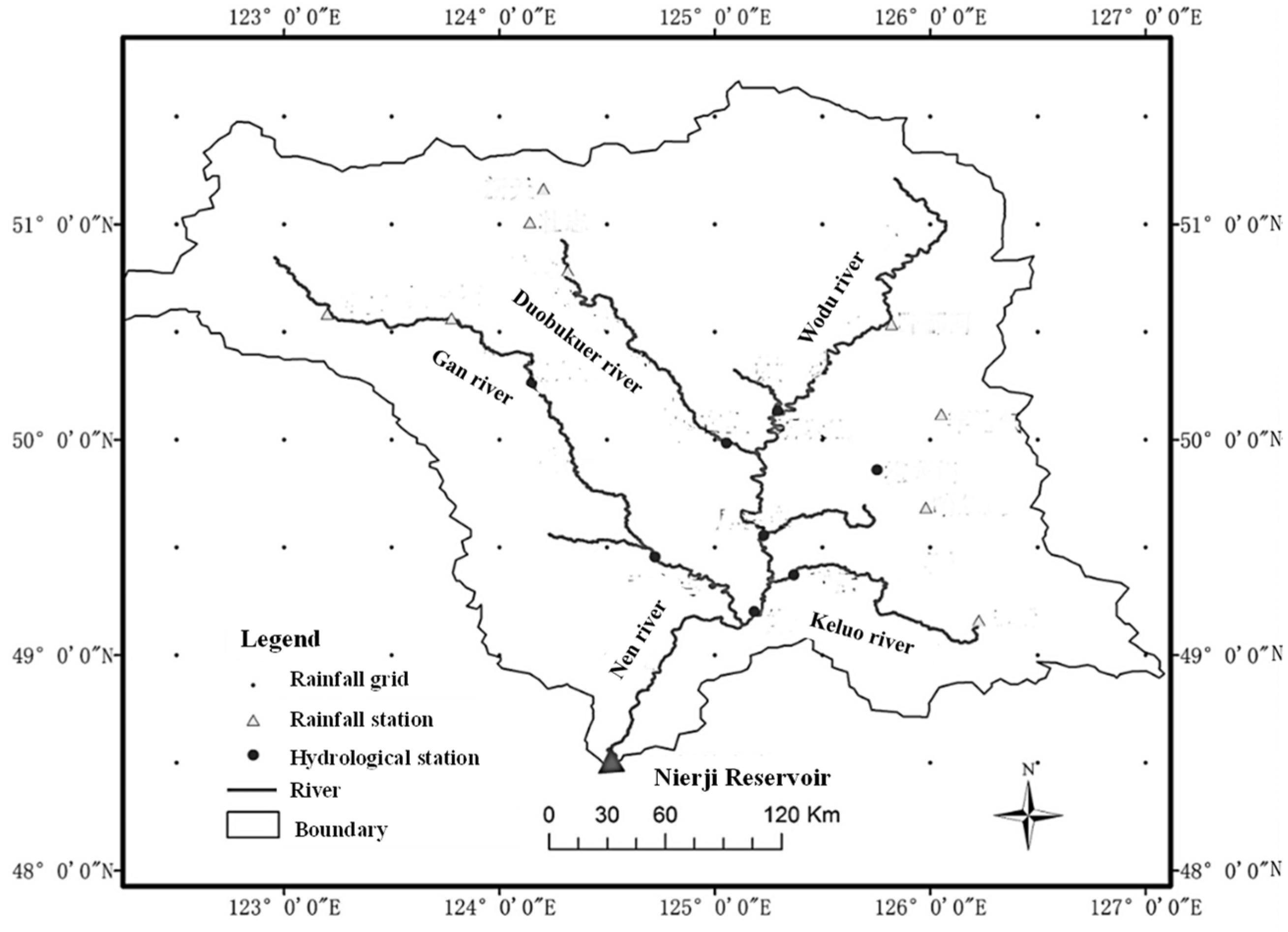
This study focuses on the parameter–simulation–optimization (PSO) framework and utilizes the non-dominated sorting genetic algorithm NSGA-II for optimization. The study constructs an operation model and applies the NSGA-II algorithm to determine various optimization variables using shared operation rule curves and independent operation rule curves as the basic operation curve forms. Additionally, the study calculates the maximum available water supply for different sectors in the reservoir through iterative calculations and uses this as a quantitative basis for comparing the water supply potential under different operation curve forms. Furthermore, multiple water demand scenarios are also designed, and the optimization method is used to obtain the Pareto solution set for each scenario. By comparing the differences in the solution sets under different operation curve forms, the study analyzes the impact of different operation curve forms on the optimization results.

2.1. Study Site

The Nierji reservoir is located in the middle reaches of the Nen River, at the border of Heilongjiang Province and the Inner Mongolia Autonomous Region (Figure 1). The hydropower station is a riverbed-type power station, equipped with four ZZA833-LH-640 type hydro turbine generators, with a single unit capacity of 62.5 MW and a total installed capacity of 250 MW, with a guaranteed output of 35 MW. The reservoir characteristics are illustrated in Tang, et al. [17]. In the study, the water demand of various sectors is set as the baseline, with industrial and domestic annual water demand at 1.029 × 10⁹ cubic meters, agricultural irrigation annual water demand at 1.646 × 10⁹ cubic meters, wetland (fish reed) annual water demand at 0.328 × 10⁹ cubic meters, and environmental annual water demand at 1.365 × 10⁹ cubic meters. This study collects daily inflow data of the reservoir from 1956 to 2015 for auxiliary runoff regulation calculations.

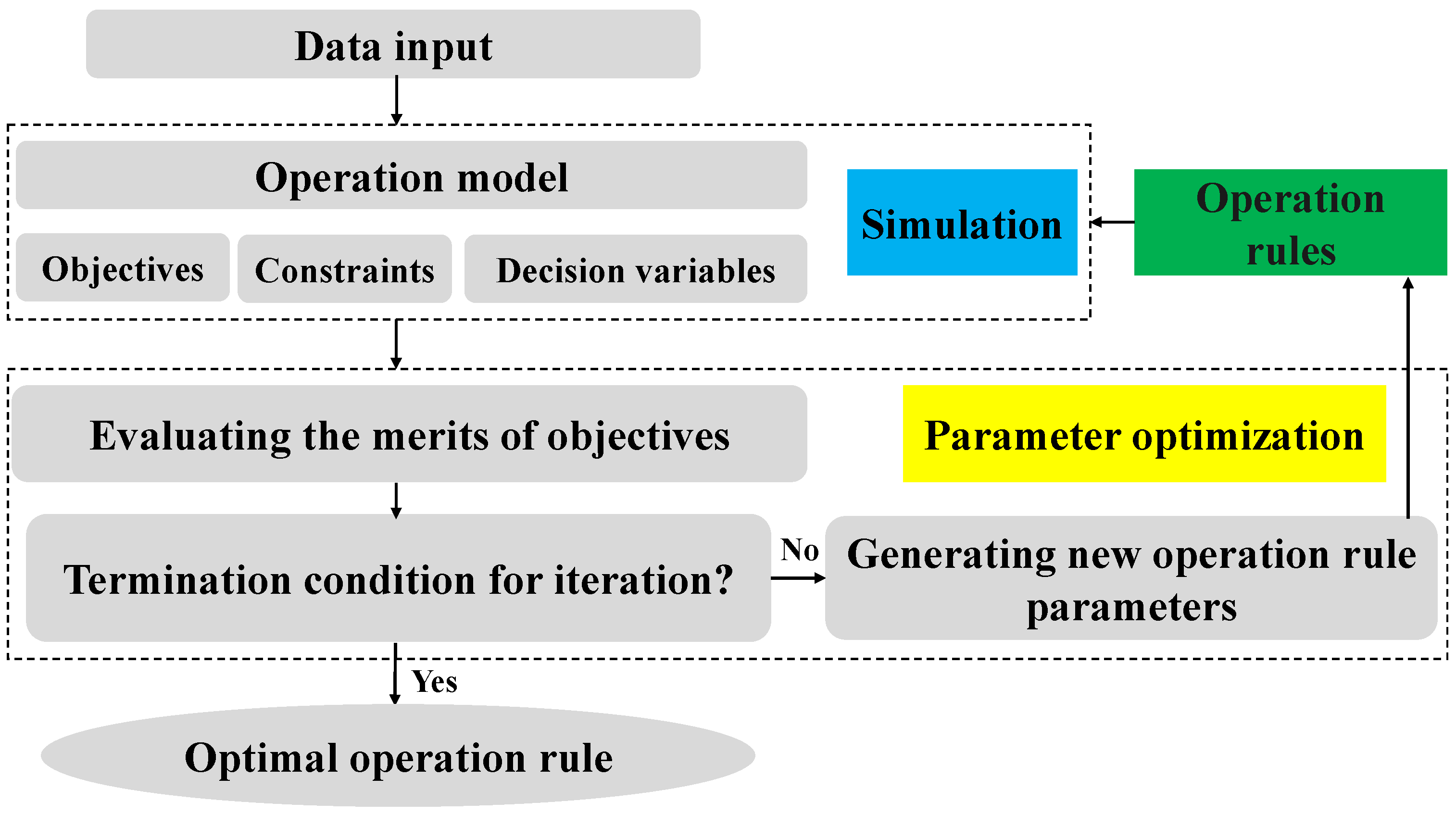
2.2. Parameter–Simulation–Optimization Framework

The method for extracting the operation curves in this study mainly adopts the widely used parameter–simulation–optimization (PSO) framework. Specifically, the optimal operation rules are obtained through an effective intelligent optimization extraction method based on the predetermined form of the operation curves. The decision variables in this method are the parameters of the reservoir operation rules, which correspond to the control points on the curves. As shown in Figure 2, the specific steps are as follows:
Generate a set of initial operation rules within the feasible range.
Simulate the reservoir’s operation process based on these operation rules and calculate relevant evaluation indicators.
Convert these indicators into fitness values that can be used by the intelligent optimization method.
Evaluate all operation rules and generate new operation rules through the intelligent optimization method.
Check if the stopping criterion is met. If it is met, the iteration process stops. Otherwise, go back to step ②.

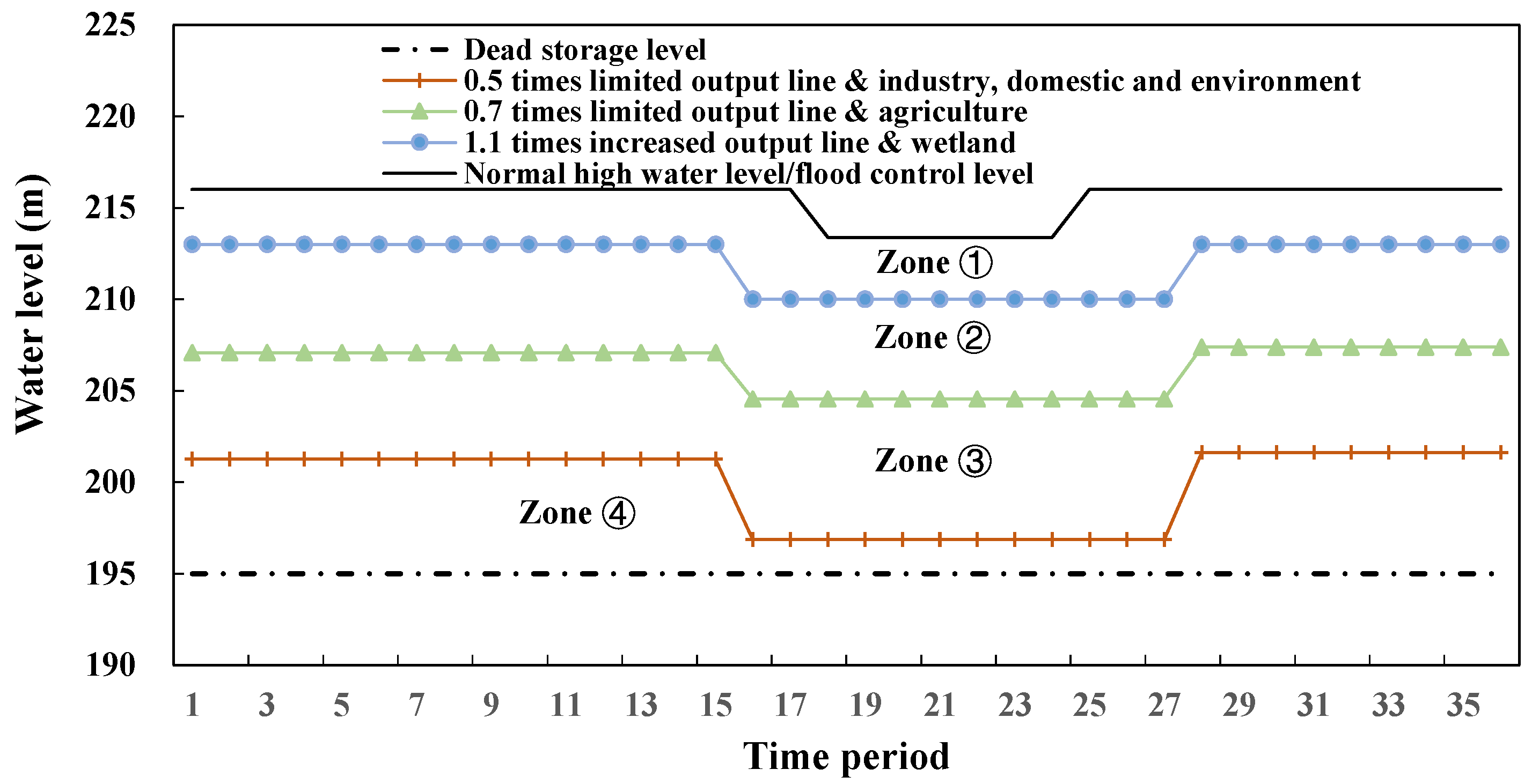
2.3. Reservoir Operation Rules

2.3.1. Independent Operation Rule Curves

In the case of the Nierji Reservoir, this study proposes an independent operation rule curve design comprising four water supply control lines for wetlands, agriculture, environment, and the combined needs of industry and domestic. Additionally, there are three power generation control lines: 1.1 times increased output line, 0.7 times limited output line, and 0.5 times limited output line. Please refer to Figure 3 for a more detailed representation.
(1)
Water supply rules
The water supply rule for each water user is determined based on the required water demand and the water supply coefficient. The water supply coefficient for each user is determined by the water level during the specific time period and the corresponding user’s water supply restriction line. If the water level is above the water supply restriction line, the water supply coefficient is 1.0; otherwise, it is reduced by a certain value. The reduction values for industrial and domestic water, environmental water, agricultural water, and wetland water (θind,t, θenv,t, θagr,t, θwet,t) are 0.9, 0.9, 0.7, and 0.5, respectively. The total water release quantity (Qs,t) for meeting the overall water supply demand is calculated as follows:
Q s , t = D i n d , t × θ i n d , t + D e n v , t × θ e n v , t + D a g r , t × θ a g r , t + D w e t , t × θ w e t , t
When the water level is in Zone 1 of Figure 3a, it indicates that the reservoir has abundant water supply, and all users are supplied according to their demand with a water supply coefficient of 1.0. When the water level is in Zone 2, the water supply for wetlands needs to be reduced. When the water level is in Zone 3, both wetlands and agriculture require a reduction in water supply. When the water level is in Zone 4, all users, except for industrial and domestic water users, need to reduce their water supply. When the water level is in Zone 5, all users need to reduce their water supply.
(2)
Hydropower generation rules
For power generation, the power output N is determined based on the water level and the power control line in Figure 3b. The required water release quantity for power generation Qe,t is also determined accordingly. The power control line divides the entire storage capacity into four zones, and the power output is equal to the guaranteed output multiplied by the power coefficient of each zone. The power coefficients for Zone I, Zone II, Zone III, and Zone IV are 1.1, 1.0, 0.7, and 0.5, respectively.
(3)
Final outflow rules
The final discharge rule is that the reservoir discharge amount Qt for each time period is the maximum value between the water release amount for water supply demand Qs,t and the water release amount for power generation demand Qe,t, i.e., Qt = max(Qs,t, Qe,t).

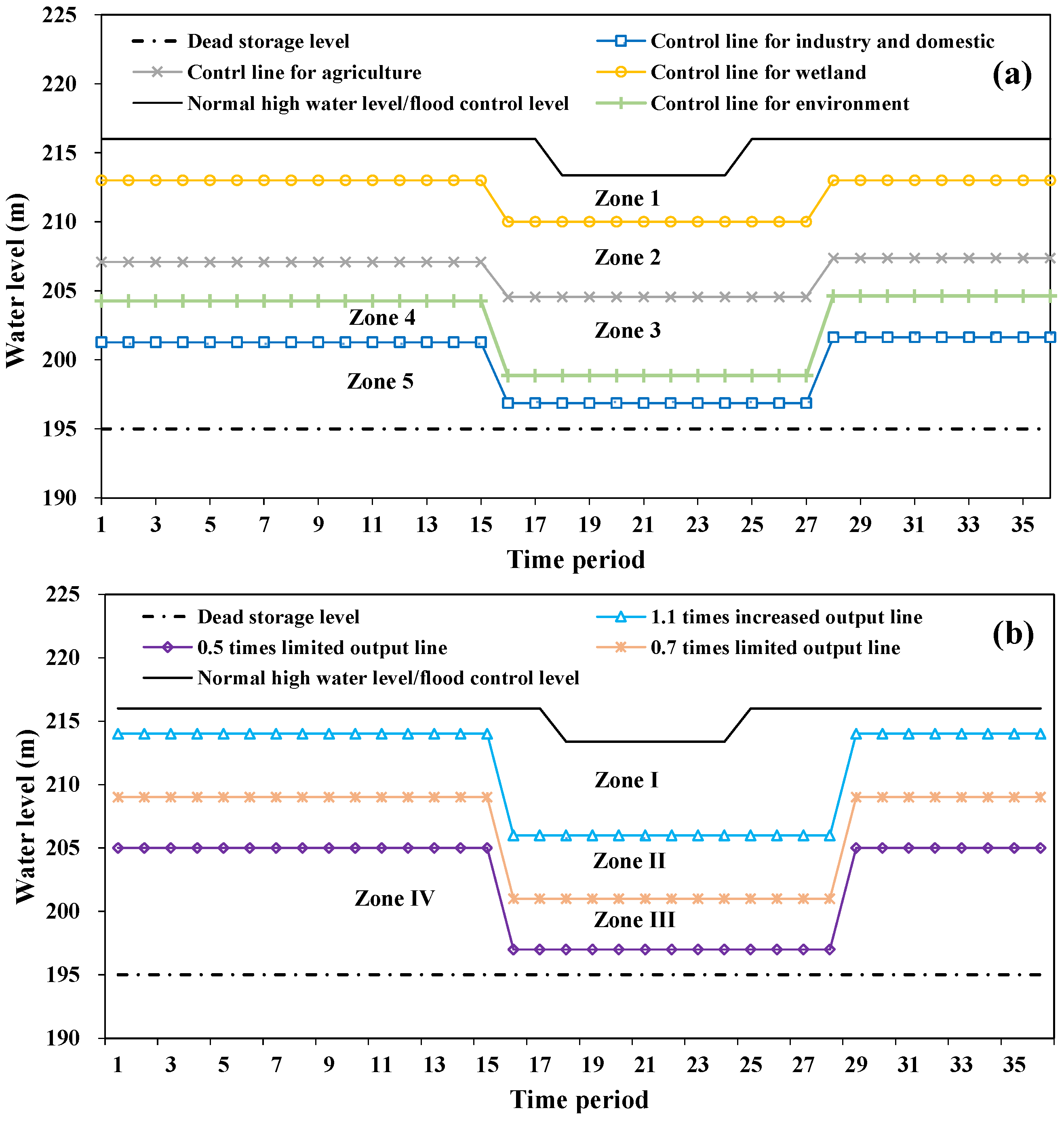
2.3.2. Shared Operation Rule Curves

For the Nierji Reservoir, the basic design of the shared operation rule curves consists of three control lines, as shown in Figure 4.
(1)
Water supply rules
For the shared operation rule curves, the total water demand and discharge volume are not different from the independent type. The main difference lies in the following: when the water level is in Zone ①, all users can be supplied according to their needs. When the water level is in Zone ②, wetland water use needs to be reduced. When the storage capacity or water level is in Zone ③, wetland and agricultural water needs to be reduced. When the storage capacity or water level is in Zone ④, water use for all users needs to be reduced.
(2)
Hydropower generation rules
For hydropower generation, the actual power output N is determined based on the water level and the position of the power generation control line. The required discharge volume for hydropower generation Qe,t is determined accordingly. When the water level is in Zone ①, Zone ②, Zone ③, and Zone ④, the output coefficients are 1.1, 1.0, 0.7, and 0.5, respectively.
(3)
Final outflow rules
The outflow volume Qt of the reservoir for each time period is determined by taking the maximum value between the water supply discharge volume Qs,t and the hydropower generation discharge volume Qe,t, i.e., Qt = max(Qs,t, Qe,t).

2.4. Reservoir Operation Model

(1)
Objective function
The operation model is primarily constructed as a multi-objective operation model, with the main objective of maximizing the reservoir’s power generation capacity (E) and minimizing the water shortage for industrial and domestic use (IND), environmental water shortage (ENV), agricultural water shortage (AGR), and wetland water shortage (WET). The objective function is as follows:
{ E = max ( i = 1 N j = 1 J N i , j × t i , j ) / N I N D = min i = 1 N j = 1 J ( D P i , j W P i , j ) / N E N V = min   i = 1 N j = 1 J ( D E i , j W E i , j ) / N A G R = min   i = 1 N j = 1 J ( D A i , j W A i , j ) / N W E T = min   i = 1 N i = 1 J ( D W i , j W W i , j ) / N
where Ni,j represents the power generation output of the reservoir in the j-th time period of the i-th year. N represents the total number of simulated years. J represents the number of operation time periods in a year, and this study considers each period to be a ten-day interval, resulting in 36 time periods per year. ti,j represents the j-th time period of year i. DPi,j and WPi,j represent the industrial and domestic water demand and supply in the j-th time period. DEi,j and WEi,j represent the environmental water demand and supply in the j-th time period. DAi,j and WAi,j represent the agricultural water demand and supply in the j-th time period. DWi,j and WWi,j represent the downstream wetland water replenishment demand and wetland water supply in the j-th time period.
(2)
Constraint condition
The main constraints include water balance constraints, reservoir capacity constraints, maximum overflow capacity constraints, power output constraints, and reliability constraints.
Water balance constraints
{ V i , j + 1 = V i , j + I i , j R i , j E L i , j S U i , j V i + 1 , 1 = V i , J
where Vi,j and Vi,j+1 represent the reservoir capacity in the j-th time period and the j+1-th time period of the i-th year. Ii,j, Ri,j, ELi,j, and SUi,j represent the inflow runoff, power generation and water supply, reservoir losses, and spillage, respectively, in the j-th time period of the i-th year. Vi,J represents the final reservoir capacity in the i-th simulated year, while Vi+1,1 represents the initial reservoir capacity in the next year.
Reservoir capacity constraints
V l o w e r V i , j V u p p e r
where Vlower and Vupper represent the dead storage capacity and the limited storage capacity, which correspond to the minimum and maximum reservoir capacities, respectively. The maximum storage capacity is the capacity corresponding to the normal high water level during non-flood periods, and the capacity corresponding to the flood limit water level during flood periods.
Maximum overflow capacity constraints
Q i , j Q m a x
where Qi,j represents the flow rate used for power generation, and Qmax represents the maximum overcurrent capability of the generator units.
Power output constraints
N i , j N m a x
where Ni,j represents the actual output, and Nmax represents the installed capacity.
Reliability constraints
R S D 95 %
R S E 90 %
R S A 75 %
R S W 75 %
R E 85 %
where RSD, RSE, RSA, RSW, and RE represent the industrial and domestic water supply guarantee rate, environmental water supply guarantee rate, agricultural water supply guarantee rate, wetland water supplement guarantee rate, and power generation guarantee rate, respectively. RSD, RSE, and RE are determined by the corresponding user satisfaction period and the total operation period, while RSA and RSW are determined by the corresponding user satisfaction year and the total operation year.
(3)
Solution methods
The decision variables for reservoir optimization are the decision control points on the operation line. The optimization solution method used is the Non-dominated Sorting Genetic Algorithm II (NSGA-II) with an elitist strategy. This method is mainly based on the principle of non-dominated sorting to divide and rank the combined population composed of parents and offspring from small to large. Firstly, the solutions in each non-dominated sorting layer are selected into the new parent population. For example, if the number of solutions in the first non-dominated sorting layer (F1) is smaller than the population size (N), solutions from the second non-dominated sorting layer (F2) are selected. If the total number of solutions selected from F2 is greater than or equal to N, the process stops. Otherwise, new layers are added until the last selected layer (Fh) can reach the population size N. After selecting solutions from F1 to Fh, the number of solutions is usually greater than N. In this case, the solutions in Fh are further sorted based on the crowding distance operator. The top-ranked solutions are selected into the new parent population to form a population with a size of N. Then, this parent population is combined with the offspring population generated through crossover and mutation to form a new combined population. This process continues until the termination condition of the algorithm is met.
Moreover, the optimal solution in the iterative calculation method is defined based on a set of predefined objectives or performance indicators. These criteria guide the iterative adjustment of the operation rule curve to improve performance in each criterion. For instance, through non-dominated sorting and crowding distance calculation, a certain number of solutions are selected from each rank as parent solutions for the current iteration. The selection process prioritizes lower ranks to retain superior solutions. Additionally, solutions with higher diversity are chosen based on crowding distance to increase solution variety. By combining these criteria, the iterative calculation method identifies superior solutions in each generation and gradually approaches the optimal solution set after multiple iterations, achieving reservoir multi-objective optimization. Furthermore, a termination condition can be set to determine convergence. This condition can be based on when the fitness values of individuals in the population no longer significantly change or when the differences between individuals are below a certain threshold. Once this condition is met, the algorithm is considered converged, and the iteration can be stopped. This approach is particularly suitable for complex problems or when there is no specific iteration limit.

3. Results and Discussion

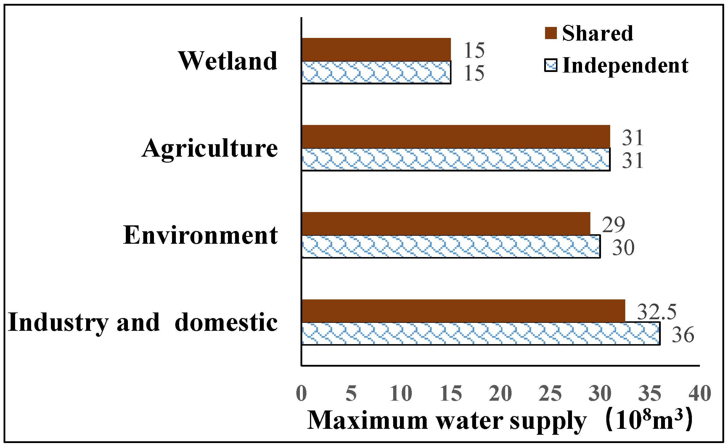
3.1. Comparison of Water Supply Potential

In the analysis of water supply potential comparison, one of the users is selected as the potential water demand development target for the future. The water demand of this user is gradually increased while keeping the water demand of other users unchanged. The objective is to determine the upper limit threshold of the potential user’s water demand, which serves as the maximum supply capacity of the reservoir for the specific user under the guarantee rate conditions of various industries. This threshold value is used to evaluate the water supply potential of the reservoir. The determination method of this threshold value is mainly based on iterative calculations. When the water demand increases to a certain value and there is an optimal solution, further increasing the water demand will not yield an optimal solution. This value is then considered as the upper limit threshold of the water demand.
Through repeated calculations and deductions, the maximum supply capacity of various users, such as industry and domestic, environment, agriculture, and wetlands in the Nierji Reservoir, is shown in Figure 5 when using independent operation and shared operation. Among them, there are differences in the maximum supply capacity of industry and domestic, and the environment. When using independent operation, the supply potential of industry and domestic, and environment users is relatively higher. Compared to shared operation, the maximum supply capacity of industry and domestic is increased by 3.5 × 10⁸ m3, a 10.8% increase, and the environment is increased by 1 × 10⁸ m3, a 3.4% increase. This is mainly because, when using independent operation, each user has independently set supply and power control lines, which leads to a wider feasible solution search space. This allows for meeting the constraints and optimizing the objectives even under greater water demand. Conversely, in shared operation, the feasible solution search space is significantly reduced due to the shared power and supply control lines. This may result in a situation where it is difficult to simultaneously meet the power guarantee rate and the guarantee rate for wetlands, agriculture, and other water supply users in the relatively small solution space. In order to satisfy the water guarantee rate of each user, the water supply potential of users will be reduced to some extent.
There is no difference in the water supply potential for agriculture and wetlands when using different basic forms of operation rule curves. This can be seen from Figure 5, where the maximum supply capacity is calculated using independent and shared operation rule curves, and it can be observed that there is no difference between the two. This is mainly because the water demand for agriculture and wetland users is more concentrated compared to industrial and environmental users, and the water demand changes mainly occur from late April to early October (the wetland replenishment period is from late August to late September, and the agricultural water demand period is from late April to early October). According to the final discharge rules, the majority of the water release from late April to early October is mainly based on the water demand for supply, as shown in Figure 6. Figure 6 shows the statistical discharge flow controlled by water demand during the selected representative years (2003 as wet, 2004 as average, and 1995 as dry) when the agricultural water demand is 31 × 108 m3 and the operation rule curves are independent and shared. From this figure, it can be observed that, regardless of which operation rule curve is used, the water release from late April to early October is mainly controlled by the water demand for supply, that is, the water supply during these periods is greater than the water release for power generation. During this time, the supply control line plays a major role in controlling the discharge, while the power control line is almost ineffective. In other periods where there is no water demand for wetlands or agriculture, the overall increase in water demand for wetlands or agriculture has no impact on the water demand during these periods. The water release during these periods is determined by the water demand of industrial and domestic, and environmental users, which is relatively small. Therefore, the power control line only plays a role during these periods. From the above analysis, it can be concluded that a shared control line is sufficient to meet the requirements for discharge control.
There are differences in the water supply potential among the various users, especially the wetland user, who has a significant difference compared to the other three users. This is because the water demand of each user varies in different time periods, particularly for wetlands, and the replenishment period is concentrated in only four decades from late August to late September. In order to meet the water supply guarantee rate requirements for wetlands, its water supply potential is severely limited.

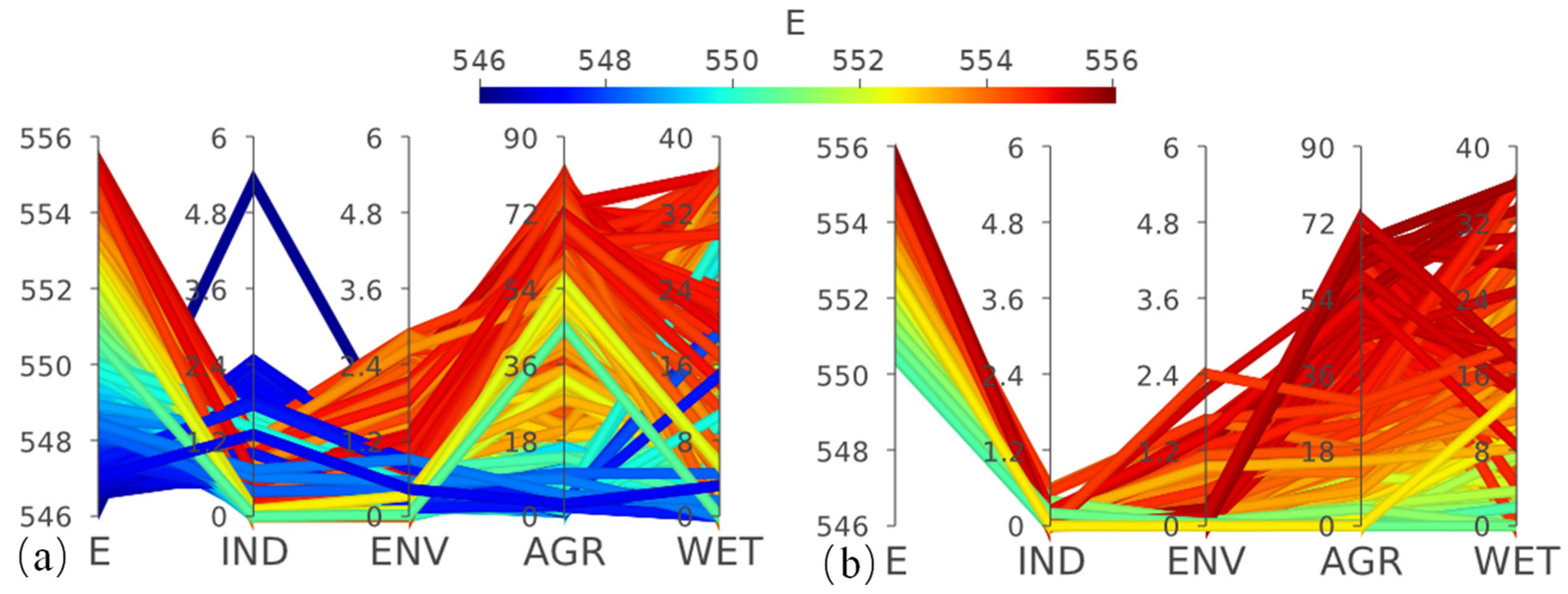
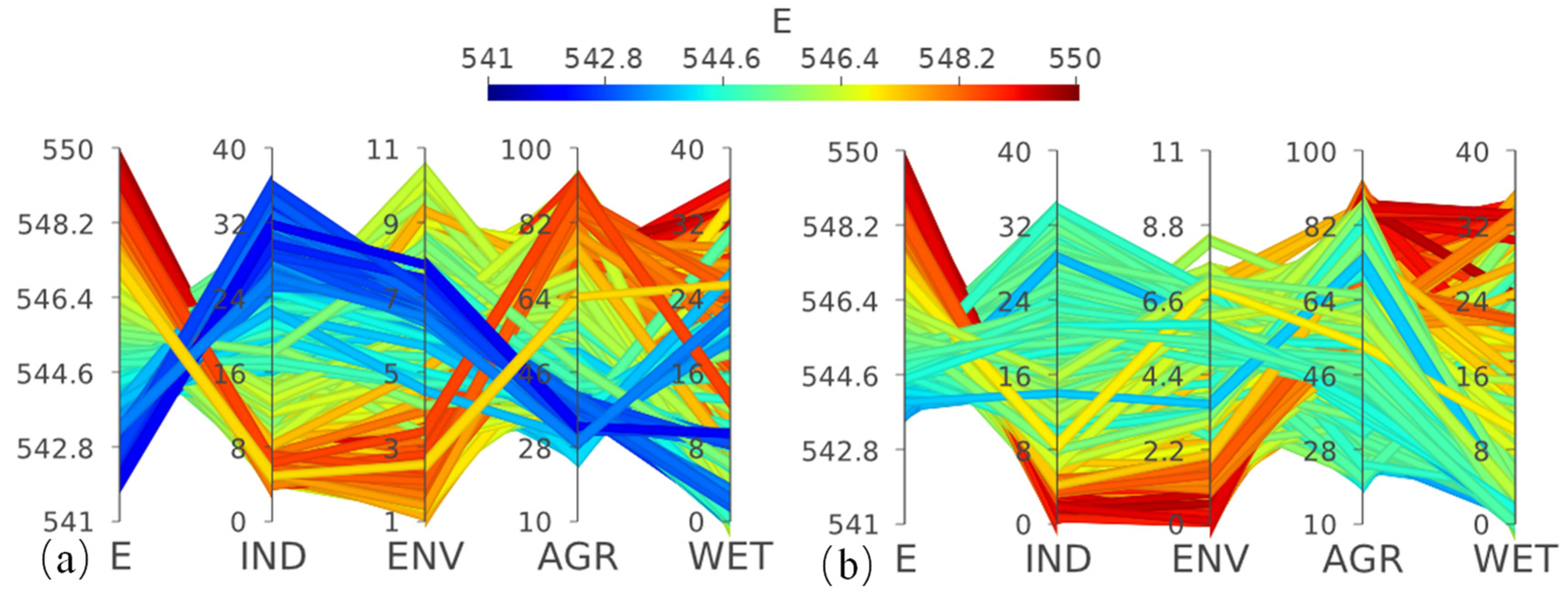
3.2. Comparison of Pareto Solution Sets for Different Operation Rule Curves in a Multi-Water Use Scenario

(1)
Designing different water demand scenarios
To further compare and analyze the impact of different basic forms of operation rule curves on the optimization results of reservoir operation, this study designs three water demand scenarios for industrial use, ranging from low to high (Table 1). The Pareto solution sets are obtained for each water demand scenario by optimizing using different basic forms of operation rule curves.
(2)
Comparison of different operation rule curves solution sets under multiple scenarios
To eliminate the influence of the randomness of genetic algorithm optimization on the results, the solution sets used for comparison in this study are obtained by performing non-dominated sorting on 10 solution sets obtained from 10 iterations of 50,000 generations. Figure 7, Figure 8 and Figure 9 show the value distribution of each objective in the solution sets obtained using two different operation rule curves under different low, medium, and high water demand scenarios. Combining the statistical results of the optimal values of each objective for different operation rule curves in Table 2 for multiple water demand scenarios, it can be seen that, under the low water demand scenario, there is little difference in the solution sets obtained using different operation rule curves. Specifically, the value ranges of each objective in the solution sets are almost the same, and the optimal values of each objective are almost identical. Under the medium water demand scenario, there is also no significant difference in the solution sets obtained using different operation rule curves, as indicated by the presence of non-dominated solutions in both types of solution sets after merging, as shown in Table 3. This indicates that, when the water demand is relatively low compared to the inflow, the water conflicts among different users are not significant, and the use of either independent or shared operation rule curves has little impact on the optimization results.
Under high water demand scenarios, the values of each objective in the solution set obtained using the shared operation rule curve are relatively concentrated. This is because the solution space of the shared operation rule curve is relatively small, resulting in a significantly smaller number of solution sets that satisfy the constraints compared to the solution sets obtained using the independent operation rule curve. As shown in Table 2, the independent operation rule curve can achieve better solutions in objectives such as power generation, industrial water use, and domestic water use. Specifically, industrial and domestic water use can be reduced by 20.1 × 10⁶ m3 and 20%, respectively. Moreover, the overall quality of the solution set obtained using the independent operation rule curve is superior to that obtained using the shared operation rule curve. After performing non-dominated sorting on the solution sets obtained using the two operation rule curves and merging them, a total of 6549 non-dominated solutions were obtained, all of which originated from the independent operation rule curve optimization. This indicates that the solutions obtained using the independent operation rule curve are superior to those obtained using the shared operation rule curve in all objectives. None of the solutions from the shared operation rule curve survived the non-dominated sorting after merging the solution sets. In scenarios where water demand is relatively high compared to inflow, water conflicts among different users become more pronounced. At this time, using the independent operation rule curve allows for a broader search space and the ability to find more optimal solutions.
The above study on reservoir operation rule curves is conducted based on the assumption of increased water usage scenarios, which did not explicitly mention the consideration of external factors such as climate change or changes in water demand patterns. This could be seen as a limitation of the proposed rule curves. Climate change can have a significant impact on water availability, inflow patterns, and reservoir operation. It can lead to changes in precipitation patterns, increased evaporation rates, and altered hydrological cycles. These changes can affect the reliability and accuracy of the proposed rule curves in the face of changing climate conditions. Similarly, changes in water demand patterns, such as population growth, urbanization, or shifts in agricultural practices, can also influence the applicability of the proposed rule curves. These changes can lead to variations in water demand, which may not be adequately addressed by the existing rule curves. Therefore, it is crucial to consider these external factors when developing reservoir operation rules. Incorporating climate change projections and assessing future water demand scenarios can provide a more comprehensive and robust approach to optimize reservoir operations. By accounting for these external factors, the proposed rule curves can be adapted or modified to ensure their continued relevance and effectiveness in the face of changing conditions.

4. Conclusions

This study focuses on determining the basic form of operation rule curves for reservoir management, considering simultaneous water supply and hydropower generation. It quantitatively analyzes the differences in water supply potential for different water users in the Nierji reservoir under two basic forms of operation rule curves: shared and independent operation rule curves. The study also compares the quality of the optimization solution sets obtained using these two forms of operation rule curves. Based on the research conducted in this study, the following main conclusions can be drawn:
(1)
The choice of operation rule curves has an impact on the maximum water supply potential of the reservoir. The independent operation rule curves show better potential for industrial, domestic, and environmental water supply compared to the shared operation rule curves. The maximum water supply for industrial and domestic purposes can be increased by 3.5 × 10⁸ m3, an improvement of 10.8%. The maximum water supply for environmental purposes can be increased by 1 × 10⁸ m3, an improvement of 3.4%.
(2)
In cases where water demand is relatively low, the shared operation rule curves can achieve similar functionality to the independent operation rule curves and yield better solution sets. By utilizing the shared operation rule curves, the number of optimization variables can be reduced by nearly half. For complex reservoir systems, analyzing the basic form of the operation rule curves can help identify common patterns among reservoirs, thus minimizing the number of optimization variables, enhancing the efficiency of the optimization process, and improving the structure of the optimization model.
(3)
When water demand is relatively high, the solution sets obtained using the independent operation rule curves are notably superior. Industrial and domestic water usage can be reduced by 20.1 × 10⁶ m3 or by 20%. The independent operation rule curve optimization yielded a total of 6549 non-dominated solutions, which were superior in overall solution quality compared to the solutions obtained through the shared operation rule curve optimization. If the goal is to maximize reservoir operation benefits, the independent operation rule curves can be employed to achieve multi-objective optimization.
Overall, this study underscores the importance of selecting appropriate operation rule curves for reservoir management. By understanding the differences between shared and independent operation rule curves, reservoir managers can make informed decisions to optimize water supply and hydropower generation, while considering the needs of various water users. However, the current research primarily focuses on the Nierji reservoir operation as an example. This case alone may not fully capture the complexity of real-world problems and the effectiveness of the corresponding results. It is important to note that some of the research findings in this study may be more evident in the context of complex reservoir group operations. Further research and analysis are necessary to better understand and address these challenges.

Author Contributions

All authors contributed to the study conception and design. Data collection and analysis were performed by R.T., J.Z., Y.W. and X.Z. The first draft of the manuscript was written by R.T. All authors have read and agreed to the published version of the manuscript.

Funding

This work was partially supported by National Natural Science Foundation of China (Grant No: 52209028, 52109001).

Data Availability Statement

The datasets generated during and/or analyzed during the current study are not publicly available due to obligation to the data provider, but are available from the corresponding author on reasonable request.

Conflicts of Interest

Author Jiabin Zhang was employed by the company of POWERCHINA Beijing Engineering Corporation Limited. The remaining authors declare that the research was conducted in the absence of any commercial or financial relationships that could be construed as a potential conflict of interest.

References

  1. Yang, G.; Guo, S.; Liu, P.; Li, L.; Xu, C. Multiobjective reservoir operating rules based on cascade reservoir input variable selection method. Water Resour. Res. 2017, 53, 3446–3463. [Google Scholar] [CrossRef]
  2. Jeuland, M.; Whittington, D. Water resources planning under climate change: Assessing the robustness of real options for the Blue Nile. Water Resour. Res. 2014, 50, 2086–2107. [Google Scholar] [CrossRef]
  3. Dabhade, P.D.; Regulwar, D.G. Sustainable Multi-Objective Multi-Reservoir Optimization Considering Environmental Flow. J. Water Resour. Prot. 2021, 13, 945–956. [Google Scholar] [CrossRef]
  4. Guo, X.; Hu, T.; Lu, Y.; Zhang, T. Multi-reservoir operating rule in inter-basin water transfer-supply project. Shuili Xuebao J. Hydraul. Eng. 2012, 43, 757–766. [Google Scholar]
  5. Peng, A.; Peng, Y.; Zhou, H.; Zhang, C. Multi-reservoir joint operating rule in inter-basin water transfer-supply project. Sci. China Technol. Sci. 2015, 58, 123–137. [Google Scholar] [CrossRef]
  6. Giuliani, M.; Galelli, S.; Soncini-Sessa, R. A dimensionality reduction approach for many-objective Markov Decision Processes: Application to a water reservoir operation problem. Environ. Model. Softw. 2014, 57, 101–114. [Google Scholar] [CrossRef]
  7. Guo, K.; Zhang, L. Multi-objective optimization for improved project management: Current status and future directions. Autom. Constr. 2022, 139, 104256. [Google Scholar] [CrossRef]
  8. Zhang, C.; Li, Y.; Chu, J.; Fu, G.; Tang, R.; Qi, W. Use of many-objective visual analytics to analyze water supply objective trade-offs with water transfer. J. Water Resour. Plan. Manag. 2017, 143, 05017006. [Google Scholar] [CrossRef]
  9. Chu, J.; Zhang, C.; Fu, G.; Li, Y.; Zhou, H. Improving multi-objective reservoir operation optimization with sensitivity-informed dimension reduction. Hydrol. Earth Syst. Sci. 2015, 19, 3557–3570. [Google Scholar] [CrossRef]
  10. Li, F.-F.; Qiu, J. Multi-objective reservoir optimization balancing energy generation and firm power. Energies 2015, 8, 6962–6976. [Google Scholar] [CrossRef]
  11. Reddy, M.J.; Nagesh Kumar, D. Multi-objective particle swarm optimization for generating optimal trade-offs in reservoir operation. Hydrol. Process. Int. J. 2007, 21, 2897–2909. [Google Scholar] [CrossRef]
  12. Matrosov, E.S.; Huskova, I.; Kasprzyk, J.R.; Harou, J.J.; Lambert, C.; Reed, P.M. Many-objective optimization and visual analytics reveal key trade-offs for London’s water supply. J. Hydrol. 2015, 531, 1040–1053. [Google Scholar] [CrossRef]
  13. Mirjalili, S.; Jangir, P.; Mirjalili, S.Z.; Saremi, S.; Trivedi, I.N. Optimization of problems with multiple objectives using the multi-verse optimization algorithm. Knowl. -Based Syst. 2017, 134, 50–71. [Google Scholar] [CrossRef]
  14. Fang, R.; Popole, Z. Multi-objective optimized scheduling model for hydropower reservoir based on improved particle swarm optimization algorithm. Environ. Sci. Pollut. Res. 2020, 27, 12842–12850. [Google Scholar] [CrossRef] [PubMed]
  15. Hu, T.; Zhang, X.-Z.; Zeng, X.; Wang, J. A two-step approach for analytical optimal hedging with two triggers. Water 2016, 8, 52. [Google Scholar] [CrossRef]
  16. Yu, Y.; Zhou, T.; Zhao, R.; Zhang, J.; Min, X. Bi-level hybrid game model for optimal operation of multi-function reservoir considering integrated water resource management. Environ. Sci. Pollut. Res. 2022, 1–18. [Google Scholar] [CrossRef] [PubMed]
  17. Tang, R.; Ding, W.; Ye, L.; Wang, Y.; Zhou, H. Tradeoff analysis index for many-objective reservoir optimization. Water Resour. Manag. 2019, 33, 4637–4651. [Google Scholar] [CrossRef]
  18. Smith, R.; Kasprzyk, J.; Zagona, E. Many-objective analysis to optimize pumping and releases in multireservoir water supply network. J. Water Resour. Plan. Manag. 2016, 142, 04015049. [Google Scholar] [CrossRef]
  19. Chang, L.-C.; Chang, F.-J. Multi-objective evolutionary algorithm for operating parallel reservoir system. J. Hydrol. 2009, 377, 12–20. [Google Scholar] [CrossRef]
  20. Woodruff, M.J.; Reed, P.M.; Simpson, T.W. Many objective visual analytics: Rethinking the design of complex engineered systems. Struct. Multidiscip. Optim. 2013, 48, 201–219. [Google Scholar] [CrossRef]
  21. Mansouri, S.; Fathian, H.; Shahbazi, A.N.; Lour, M.A.; Asareh, A. Multi objective simulation–optimization operation of dam reservoir in low water regions based on hedging principles. Environ. Sci. Pollut. Res. 2023, 30, 41581–41590. [Google Scholar] [CrossRef] [PubMed]
  22. Liu, P.; Guo, S.; Xu, X.; Chen, J. Derivation of aggregation-based joint operating rule curves for cascade hydropower reservoirs. Water Resour. Manag. 2011, 25, 3177–3200. [Google Scholar] [CrossRef]
  23. Ahmadi Najl, A.; Haghighi, A.; Vali Samani, H.M. Simultaneous optimization of operating rules and rule curves for multireservoir systems using a self-adaptive simulation-GA model. J. Water Resour. Plan. Manag. 2016, 142, 04016041. [Google Scholar] [CrossRef]
  24. Li, Y.; Ding, W.; Chen, X.; Cai, X.; Zhang, C. An analytical framework for reservoir operation with combined natural inflow and controlled inflow. Water Resour. Res. 2020, 56, e2019WR025347. [Google Scholar] [CrossRef]
  25. Yang, S.; Yang, D.; Chen, J.; Zhao, B. Real-time reservoir operation using recurrent neural networks and inflow forecast from a distributed hydrological model. J. Hydrol. 2019, 579, 124229. [Google Scholar] [CrossRef]
  26. Khadr, M.; Schlenkhoff, A. GA-based implicit stochastic optimization and RNN-based simulation for deriving multi-objective reservoir hedging rules. Environ. Sci. Pollut. Res. 2021, 28, 19107–19120. [Google Scholar] [CrossRef] [PubMed]
  27. Ahmadianfar, I.; Samadi-Koucheksaraee, A.; Razavi, S. Design of optimal operating rule curves for hydropower multi-reservoir systems by an influential optimization method. Renew. Energy 2023, 211, 508–521. [Google Scholar] [CrossRef]
  28. Moeini, R.; Hadiyan, P.P. Hybrid methods for reservoir operation rule curve determination considering uncertain future condition. Sustain. Comput. Inform. Syst. 2022, 35, 100727. [Google Scholar] [CrossRef]
  29. El Harraki, W.; Ouazar, D.; Bouziane, A.; Hasnaoui, D. Optimization of reservoir operating curves and hedging rules using genetic algorithm with a new objective function and smoothing constraint: Application to a multipurpose dam in Morocco. Environ. Monit. Assess. 2021, 193, 196. [Google Scholar] [CrossRef]
  30. SeethaRam, K.V. Three Level Rule Curve for Optimum Operation of a Multipurpose Reservoir using Genetic Algorithms. Water Resour. Manag. 2021, 35, 353–368. [Google Scholar] [CrossRef]
  31. Kosasaeng, S.; Yamoat, N.; Ashrafi, S.M.; Kangrang, A. Extracting Optimal Operation Rule Curves of Multi-Reservoir System Using Atom Search Optimization, Genetic Programming and Wind Driven Optimization. Sustainability 2022, 14, 16205. [Google Scholar] [CrossRef]
  32. Takada, A.; Hiramatsu, K.; Trieu, N.A.; Harada, M.; Tabata, T. Development of an optimizing method for the operation rule curves of a multipurpose reservoir in a Southeast Asian watershed. Paddy Water Environ. 2019, 17, 195–202. [Google Scholar] [CrossRef]
  33. Ngoc, T.A.; Hiramatsu, K.; Harada, M. Optimizing the rule curves of multi-use reservoir operation using a genetic algorithm with a penalty strategy. Paddy Water Environ. 2014, 12, 125–137. [Google Scholar] [CrossRef]
  34. Ahmadianfar, I.; Samadi-Koucheksaraee, A.; Asadzadeh, M. Extract nonlinear operating rules of multi-reservoir systems using an efficient optimization method. Sci. Rep. 2022, 12, 18880. [Google Scholar] [CrossRef]
  35. Ahmadianfar, I.; Kheyrandish, A.; Jamei, M.; Gharabaghi, B. Optimizing operating rules for multi-reservoir hydropower generation systems: An adaptive hybrid differential evolution algorithm. Renew. Energy 2021, 167, 774–790. [Google Scholar] [CrossRef]
  36. Chen, L.; McPhee, J.; Yeh, W.W.G. A diversified multiobjective GA for optimizing reservoir rule curves. Adv. Water Resour. 2007, 30, 1082–1093. [Google Scholar] [CrossRef]
  37. Tang, R.; Li, K.; Ding, W.; Wang, Y.; Zhou, H.; Fu, G. Reference point based multi-objective optimization of reservoir operation: A comparison of three algorithms. Water Resour. Manag. 2020, 34, 1005–1020. [Google Scholar] [CrossRef]
Figure 1. Study site.
Water 16 00276 g001
Figure 2. Flowchart of the framework for parameterization, simulation, and optimization methods.
Water 16 00276 g002
Figure 3. The basic form of an independent type operation rule curve for the Nierji reservoir. (a) for water supply rules and (b) for hydropower generation rules.
Water 16 00276 g003
Figure 4. The basic form of a shared type operation rule curve for the Nierji reservoir.
Water 16 00276 g004
Figure 5. Maximum water supply for different sectors under different operation rule curves.
Water 16 00276 g005
Figure 6. Time periods of controlled outflow based on water supply demand for wet, normal, and dry typical years.
Water 16 00276 g006
Figure 7. Comparison of Pareto solution sets for different operation rule curves in a low water use scenario: (a) shared type; (b) independent type. Note: The units for E are 106 kWh, and the units for IND, ENV, AGR, and WET are in 106 m3.
Water 16 00276 g007
Figure 8. Comparison of Pareto solution sets for different operation rule curves in a medium water use scenario: (a) shared type; (b) independent type.
Water 16 00276 g008
Figure 9. Comparison of Pareto solution sets for different operation rule curves in a high water use scenario: (a) shared type; (b) independent type.
Water 16 00276 g009
Table 1. Multiple water demand scenarios.
ScenarioAnnual Water Demand (108 m3)E (MW)
Industry and DomesticEnvironmentAgricultureWetlands
S1 (Low)10.2913.6516.463.2835
S2 (Medium)20
S3 (High)32.5
Table 2. Statistical analysis of optimal values for different objectives in various operation rule curves for multiple water demand scenarios.
ScenarioCurve FormEINDENVAGRWET
S1 (D_ind = 10.29)Shared555.340.000.000.900.00
Independent555.700.000.000.000.00
S2 (D_ind = 20)Shared549.643.841.1525.000.00
Independent549.570.480.0419.920.00
S3 (D_ind = 32.5)Shared539.1792.4821.4899.0031.84
Independent541.1372.3816.1677.833.48
Table 3. Statistical analysis of the sources of non-dominating solutions under non-dominating operation in the union and solution sets of two operation rule curves.
ScenarioCurve FormNo. of Non-Dominated Solutions
S1 (D_ind = 10.29)Shared24
Independent574
S2 (D_ind = 20)Shared1131
Independent3258
S3 (D_ind = 32.5)Shared0
Independent6549
Disclaimer/Publisher’s Note: The statements, opinions and data contained in all publications are solely those of the individual author(s) and contributor(s) and not of MDPI and/or the editor(s). MDPI and/or the editor(s) disclaim responsibility for any injury to people or property resulting from any ideas, methods, instructions or products referred to in the content.

