Comparative Evaluation of Deep Learning Techniques in Streamflow Monthly Prediction of the Zarrine River Basin

Abstract

Predicting monthly streamflow is essential for hydrological analysis and water resource management. Recent advancements in deep learning, particularly long short-term memory (LSTM) and recurrent neural networks (RNN), exhibit extraordinary efficacy in streamflow forecasting. This study employs RNN and LSTM to construct data-driven streamflow forecasting models. Sensitivity analysis, utilizing the analysis of variance (ANOVA) method, also is crucial for model refinement and identification of critical variables. This study covers monthly streamflow data from 1979 to 2014, employing five distinct model structures to ascertain the most optimal configuration. Application of the models to the Zarrine River basin in northwest Iran, a major sub-basin of Lake Urmia, demonstrates the superior accuracy of the RNN algorithm over LSTM. At the outlet of the basin, quantitative evaluations demonstrate that the RNN model outperforms the LSTM model across all model structures. The S3 model, characterized by its inclusion of all input variable values and a four-month delay, exhibits notably exceptional performance in this aspect. The accuracy measures applicable in this particular context were RMSE (22.8), R² (0.84), and NSE (0.8). This study highlights the Zarrine River’s substantial impact on variations in Lake Urmia’s water level. Furthermore, the ANOVA method demonstrates exceptional performance in discerning the relevance of input factors. ANOVA underscores the key role of station streamflow, upstream station streamflow, and maximum temperature in influencing the model’s output. Notably, the RNN model, surpassing LSTM and traditional artificial neural network (ANN) models, excels in accurately mimicking rainfall–runoff processes. This emphasizes the potential of RNN networks to filter redundant information, distinguishing them as valuable tools in monthly streamflow forecasting.

1. Introduction

Streamflow forecasting and simulation of precipitation runoff are crucial components of water resource planning and management [1], such as reservoir planning and flood risk control [2,3]. Generally, the simulation of the rainfall–runoff process encompasses two branches: methods grounded in physics and empirical techniques [4]. The first type of methods, demonstrated by process-driven techniques, need to understand the physics of hydrological processes and use linear equations and partial differential equations [4,5,6]. However, the second type of methods, demonstrated by data-driven techniques including machine learning models, do not require the knowledge of physical process and build a direct relationship between rainfall and runoff as the input and output [7]. Various models, such as autoregressive moving average (ARMA), autoregressive integrated moving average (ARIMA), and autoregressive (AR), utilize linear relationships between output and input to forecast runoff, according to a number of studies [8,9,10].

For runoff forecasting, machine learning models, which are a sub-set of data-driven techniques, are widely implemented. The utilization of support vector machines (SVM) and artificial neural networks (ANN) as machine learning models for runoff prediction has been the subject of several studies [11,12,13,14,15].

The artificial neural network (ANN) has excellent capability in nonlinear hydrologic models [16,17]. ANNs have the ability to identify nonlinear links between model inputs and model outputs, as well as recreate extremely nonlinear interactions. This is particularly useful in situations where the nonlinear relationships in question are unknown [18]. For a long time-series, overfitting [19] and converging to local least squares [20], which are both disadvantages associated with ANNs, make it tough to attain a desired prediction performance in hydrological modeling. This is the case despite the fact that ANNs are widely used [16].

In addition, a support vector machine (SVM) may find a solution that is globally optimal for classification or regression challenges. So, it could be an excellent tool in the hydrological modeling and management of water resources [1,21]. Nevertheless, SVM abilities could be restricted in practical applications due to the fact that its predicting outcomes are heavily reliant on the computational parameters that are selected [14]. Such methods can successfully reflect the nonlinearity relationships of the rainfall–runoff method which is considered among the one advantage that such models generally provide [22]. Nevertheless, one of the drawbacks associated with these machine learning methodologies is that they will have difficulty when the behavior of the system is controlled by the environment of either space or time [23,24].

In a nutshell, a machine learning model is a way of “mapping” certain input data to some desired outcomes. In order to access the full array of traditional nonlinear and linear links of such methods, the data must first be reframed before proceeding with time series forecasting [7]. The sliding window approach is often used to accomplish this goal. In the context of time series data analysis, it is customary to employ the variables from the preceding step as inputs and the variables from the subsequent step as outputs. Thus, the time series dataset is restructured as a machine learning problem in which the value at the preceding time step is utilized to predict the value at the subsequent time step [7]. The adjustable parameter is the time step utilized in the sample creation process. This choice will have an effect on the subsequent training of the model. Without any previous information, determining the best time step to take might be a challenging task. For runoff forecasting with machine learning methods, one must first determine the influence that time step selection has on runoff forecasting in order to reach the highest possible level of forecast accuracy. Recent years have witnessed an explosion in the development of deep learning technologies, including long short-term memory (LSTM), gated recurrent unit (GRU), and recurrent neural networks (RNN). This development has provided insight into how to simplify the resolution of this issue.

A significant proportion of deep learning methodologies possess the capability to analyze extensive sequences of data. One example of this is the recurrent neural network, also known as an RNN. It has been shown that an RNN is a useful tool for dealing with sequence data in order to make predictions about time series [25]. It is crucial to acknowledge that the performance of the standard implementation of an RNN does not show a substantial improvement in sequence prediction as a result of the intrinsic issue of disappearing or bursting gradients that it has. LSTM networks with an enhanced variant of an RNN have been shown to be capable of resolving the issue [7,26]. LSTM can capture not only the periodic patterns of time series data but also the chaotic ones, and they can learn their long-range links with better precision than conventional NNs are able to [27].

Both LSTM and RNNs have recently received a lot of interest from academics working in the water field. The water levels of a sanitary sewer structure in Drammen, Norway, were simulated and predicted through the utilization of online data obtained from rain gauges and water level sensors [28]. To ascertain the architecture of NNs with the most effective capability to simulate and forecast water levels, they conducted a comparative analysis of their performance. They were able to demonstrate conclusively that conventional designs that lacked explicit cell memory were not as well adapted for making multi-step-ahead predictions as LSTM and other recurrent neural network architectures that have cell memory. For the purpose of estimating future groundwater levels, the LSTM was used by Zhang et al. [29]. The simulation produced by the LSTM-based technique was evaluated with a CNN (conventional neural network), and the results showed significant improvements for the former. Utilizing the Soil and Water Assessment Tool (SWAT), Wang et al. [30] analyzed the hydrological response to the downscaled weather data after statistically downscaling meteorological data with an RNN. There has been recent research on runoff prediction utilizing LSTM, RNNs, and GRUs [6,7,31,32].

Among the issues that must be addressed by a variety of corporations and legislators in Iran is integrated water resource management [33]. For this purpose, the accuracy of streamflow prediction plays a key role, which is represented in some studies. Zhihua et al. [34] used the SWAT and ANN models for runoff prediction. The Baliqlu Chai Watershed, located in Ardabil province, was chosen as the study area. Furthermore, the error in the ANN was reduced in this study by employing an optimization method based on the mutated model of the whale optimization algorithm (MWOA). In the study [35] by Sarzaeim et al., the utilization of data-mining techniques, such as support vector machines (SVMs), genetic programming (GP), and artificial neural networks (ANNs), proved advantageous in forecasting runoff in the Aidoghmoush basin amidst climate change circumstances. The research in [36] presented a model based on the combination of genetic algorithms and the Levenberg–Marquardt (LM) algorithm to improve forecasting results. The model was proposed in the Aghchai watershed located in Azerbaijan province as the study area, and the results indicated the accuracy of the proposed method for runoff prediction in comparison with an ANN and the adaptive neuro-f inference system (ANFIS). A robust hybrid model (W-WRELM) was constructed through the integration of the wavelet transform (WT) to simulate precipitation runoff data from 2000 to 2017 in the Shaharchay River basin, which is a significant source of water for Lake Urmia in the province of Azarbayjane-Gharbi. The model spanned a duration of 18 years [37].

Drawing insights from an extensive literature review, the identification of utilizing deep learning methods for streamflow forecasting in the nuanced context of Iranian rivers underscores a key research gap. The current scientific landscape predominantly relies on established methodologies, and introducing the application of advanced techniques, specifically an RNN and LSTM, in this specific setting offers a compelling opportunity to advance hydrological research. By investigating the specific challenges and intricacies of the Zarrine River basin, which is the most expansive and significant sub-basin of Lake Urmia in Iran, this study aims to not just fill a research gap but to forge new pathways in advancing our understanding of hydrological processes in Iranian distinct geographical context.

In addition, streamflow prediction models are beset by a substantial degree of uncertainty due to the scarcity of accessible data and the intricacy of the water distribution and management network. The presence of nonoptimal model parameters, which can be challenging to evaluate directly, systematic or measurement errors in the input dataset, and a statistical model that is oversimplified and based on assumptions all contribute to the presence of uncertainty [38,39]. The uncertainties in streamflow forecasting have been the subject of a great number of studies which have been used to quantify and estimate them [39,40,41]. Both Zhang et al. [42] and Her et al. [43] came to the same conclusion, that the uncertainty in the input plays an important role in determining how accurate the streamflow prediction model is. As the most fundamental input to the rainfall–runoff model, imprecise spatial and temporal estimations of precipitation or errors in their assessment may introduce significant uncertainty into the streamflow prediction [39].

There have been numerous investigations that have used a variety of methods to quantify the uncertainty in the streamflow forecasting models [44,45,46]. Among these approaches, we benefited from the one-way analysis of variance (ANOVA) as an uncertainty analysis method to evaluate the effects of input data at each ZR station on the results. By subjecting the model to different values of input parameters and analyzing the resulting variations in the model’s output, sensitivity analysis offers significant insights regarding the model’s resilience and dependability. This information is crucial for making informed decisions, optimizing processes, and enhancing the predictive accuracy of models. As many studies have highlighted, one-way ANOVA sensitivity analysis can reveal critical input parameters that require closer attention and fine-tuning, ultimately contributing to more effective decision making and problem solving in various fields.

This research aims to evaluate and compare the performance of recurrent neural networks (RNNs) and long short-term memory (LSTM) models for monthly streamflow prediction in the Zarrine River basin, northwest Iran. The objectives include assessing model effectiveness, determining the optimal structure among five configurations, and identifying key parameters’ impact on predictions. Hypotheses anticipate better accuracy in prediction by machine learning techniques, especially in replicating monthly streamflow patterns. These objectives and hypotheses collectively aim to enhance our understanding of deep learning applications in hydrological modeling within the specific environmental context of the Zarrine River basin.

In order to ascertain the precise significance of this work, a topic evaluation is conducted utilizing the R Studio and Scopus databases (Bibliometrix library). Streamflow prediction using machine learning approaches and sensitivity analysis are not heavily considered by researchers, as indicated by the keyword assessments (Figure 1a); hence, this concept can be regarded as innovative. Furthermore, water management, artificial intelligence, streamflow prediction, and machine learning are prevalent topics within scientific communities. However, as shown in Figure 1b, neither Iranian enterprises nor researchers have made significant advancements in these areas. As a result, senior-level managers in Iran should assess the results of the current investigation as an innovative resolution.

ANOVA (analysis of variance) is crucial in this research for assessing the significance and impact of different variables on streamflow prediction models. It helps identify the key factors influencing streamflow forecasts, enhancing the accuracy of hydrological analyses.

With regard to the forecast of monthly streamflow via machine learning algorithms like an RNN and LSTM, ANOVA serves as a valuable tool to quantify the influence of various hydrological parameters. This statistical technique aids in distinguishing which variables, such as station streamflow, upstream station streamflow, and maximum temperature, significantly affect the model’s output. ANOVA’s contribution lies in pinpointing the most influential factors, thereby improving the precision and reliability of streamflow predictions in water resource management and hydrological analysis.

In spite of the increased attention recently given to the application of machine learning methods such as LSTM and RNNs in streamflow prediction, the comparative performance of these models in the context of streamflow forecasting remains an area that requires further investigation. Specifically, there is limited research that systematically evaluates and compares the predictive accuracy and suitability of RNNs and LSTM models for streamflow forecasting, particularly in the context of the Zarrine River basin in Iran. Additionally, there is a need for more in-depth exploration of the key hydrological variables that influence streamflow predictions using these models.

This research aims to assess the performance of two machine learning models, an RNN and LSTM, in streamflow prediction for the Zarrine River basin in northwest Iran. This study aims to determine which model provides more accurate predictions and identify the most influential hydrological variables. This research aims to improve streamflow prediction methods for effective water resource management in the region.

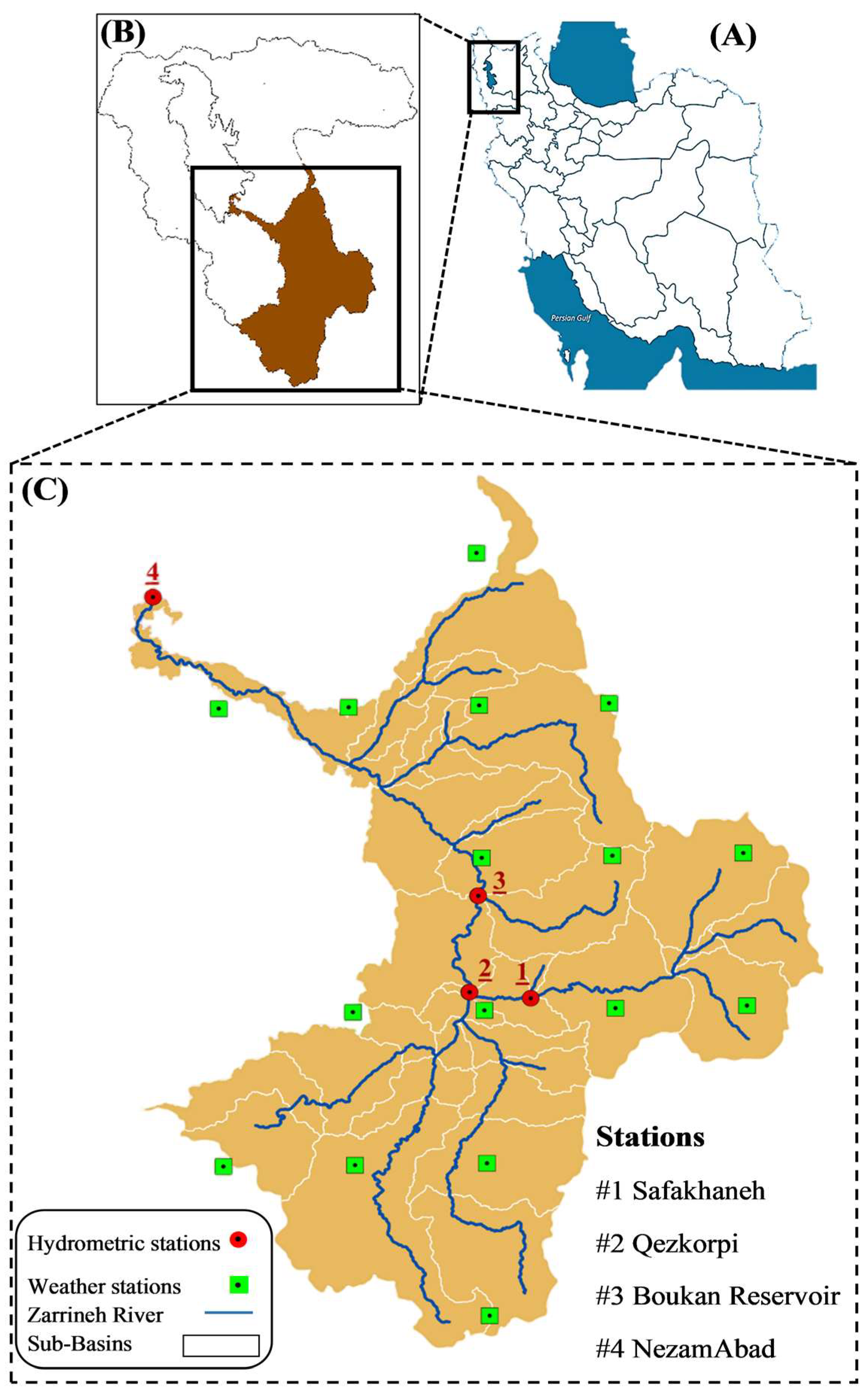
2. Data Collection and the Study Area

Lake Urmia (LU) is the largest body of water in Iran, which covers around 5750 km² and contains roughly 7% of Iran’s surface water [47]. Around 41% of the environmental discharge into the LU basin originates in the Zarrine River (ZR), making it the most substantial and sizable sub-basin of the LU basin [48]. As is evident in Figure 2, the ZR extends for a total distance of almost 300 kilometers and has an area of around 12,025 square kilometers to the southeast of the Lake Urmia [49]. With a storage capacity of 650 MCM, the Bookan Dam is the most sizable and consequential operational dam in the ZR basin. It stores water for human use, agriculture, and industry [50]. During the previous four decades, this basin has received 352 mm of precipitation annually on average, making it a semiarid area with a Mediterranean climate.

In this research, four hydrological stations were taken into account in the Zarrine River basin (see Figure 2). The statistics for the reservoir outflow and the monthly streamflow were taken from the websites www.yekom.com (Reservoir outflow statistics (Yekom Ltd., Tabriz, Iran)) and www.dams.wrm.ir (Not accessible with non-Iranian IP), respectively, for the years 1974–2014. In addition, we gathered meteorological information from the Iran Meteorological Organization, such as rainfall and high and low temperatures from 1974 to 2014.

A holistic analysis of the physical mechanisms influencing streamflow in the Zarrine River basin involves considering geographical, climatic, hydrological, anthropogenic, and topographical factors. According to Yazdandoost et al. [48], the analysis of geographical and climatic variances within the provinces reveals significant influences on hydrological processes. Variations in elevation, slope, and land cover contribute to distinct streamflow patterns in each sub-basin. Land use/cover data for 2017 showcases the impact of human activities on the basin, prompting an examination of correlations between land use patterns and observed streamflow variations over time. Hydrological connectivity within the Zarrine River basin is crucial to understanding streamflow dynamics. Factors such as soil type, derived from the Food and Agriculture Organization of the United Nations (FAO) Soil Map of the World archive, play a role in shaping hydrological responses. Assessing the variations in soil properties provides insights into how different regions contribute to the overall efficiency of streamflow prediction models. Meteorological data obtained from four stations, including Zarrine, Saqez, Takab, and Maragheh, allow for an analysis of seasonal and climatic influences. Evaluating variations in maximum and minimum daily temperatures and precipitation helps discern distinct seasonal patterns in streamflow. Additionally, the presence of the Boukan Dam, the largest water management infrastructure on the Zarrine River, with a gross storage capacity of 760 MCM (million cubic meters), influences streamflow and contributes to the mean flow rate of 139.5 MCM. Agricultural activities, outlined by information from the Iranian Ministry of Agriculture Jihad (IMAJ), introduce another layer of complexity. Cropping patterns, planting and harvesting dates, and irrigation management directly impact streamflow dynamics. The cultivated area of major crops in the Zarrine River basin further influences water usage and runoff patterns. Utilizing the digital elevation model (DEM) with a spatial resolution of 30 m × 30 m, the topography of the region is analyzed. Steep slopes, high elevations, and other topographical features contribute to variations in streamflow, influencing the overall hydrological response. Examining runoff data from hydrometric stations and reservoir outflow data provides valuable insights into the variations in streamflow at the outlets of representative sub-basins. These observations contribute to understanding the role of different factors in shaping the observed runoff patterns in the Zarrine River basin [48].

3. Model Description

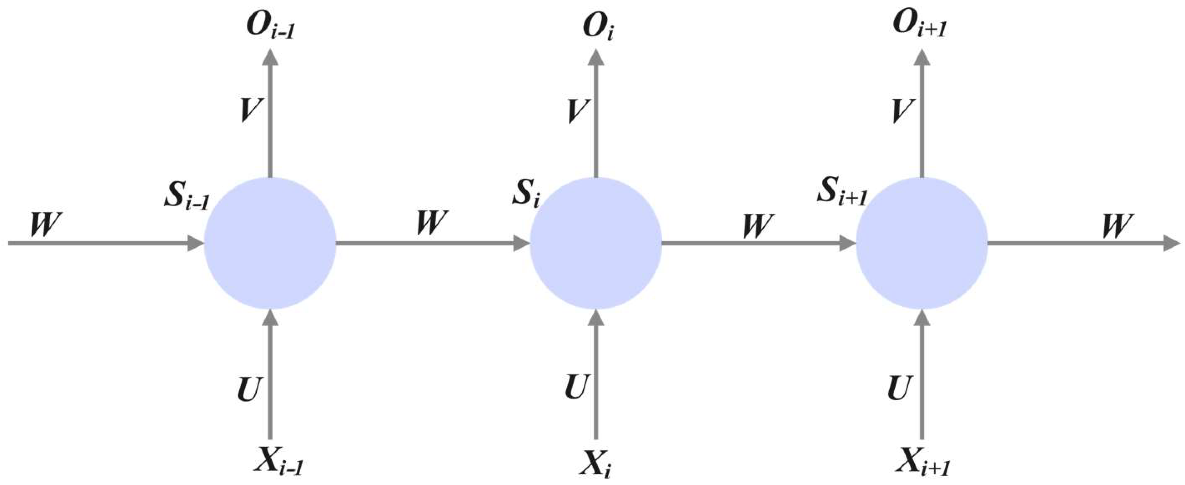
3.1. RNN (Recurrent Neural Network)

While regular neural networks have full relationships between layers, there is no communication between nodes in the same layer. In a spatial–temporal network, there are relationships between the nodes, which means that this type of network could fail when attempting to solve temporal–spatial problems. In an RNN, unlike in traditional networks, the hidden units are fed back information about how the current state compares to the previous state [51].

Figure 3 shows a simple RNN cell over two iterations. In this configuration, the RNN accepts input vectors, one at a time rather than using a fixed number of input vectors, as is the case in more conventional network architectures. Furthermore, all of the input data that have been gathered up to this point can be utilized by this architecture. Furthermore, the depth of the RNN can be adjusted without regard to the theoretical application. As demonstrated by Zhao et al. [52], the output of each subsequent hidden layer influences the ultimate result.

By using the network’s depth as an approximation of time, an RNN can simulate the correlation present in sequential data. However, the vanishing and bursting gradient problems make the RNN model less accurate as the time span becomes longer, which affects the final output [52]. Mathematically, the RNN model shown in Figure 3 can be represented as follows:

p_i = S (W₁X_i + W₂X_i−1 + b₁)

(1)

r_i = W₃p_i + b₂

(2)

ö = S (r_i)

(3)

$$\mathrm{cf}={\sum }_{\mathrm{i}}(‖\mathrm{ö}-\mathrm{o}‖/2)$$

(4)

where p_i and r_i are the temporary variables. X_i is the input variable, W₁, W₂, and W₃ are weight matrixes, b₁ and b₂ are bias vectors, S is sigmoid function, cf is the cost function, and ö and o are the expected and actual output, respectively. The sigmoid function (σ) is a mathematical function commonly used in neural networks to introduce nonlinearity. It squashes input values to a range between 0 and 1, facilitating gradient-based optimization. Temporary variables (p_i and r_i) play roles in our model’s computations. pi denotes the input gate activation, controlling the extent of input information to be stored, and r_i represents the reset gate activation, influencing the extent to which the previous state is neglected. Another fundamental aspect is backpropagation which is a crucial aspect of training neural networks. It involves iteratively adjusting the model’s parameters using the chain rule of calculus to minimize the difference between predicted and actual outputs.

Additionally, the backpropagation through time approach (BPT) can be used to train the RNN model through the utilization of a gradient calculation, where the cost corresponding to the input weights and hidden weights of the previous time steps is determined. However, the partial derivative error increases with each successive time step when using the BPTT approach. A gradient will either vanish entirely if the time step T is enormous, or it will explode enormously. The term “vanishing/exploding gradient problem” is often used to describe this issue [6]. In order to prevent vanishing/exploding gradients, LSTM or GRU blocks have largely replaced the hidden block in RNNs in recent years.

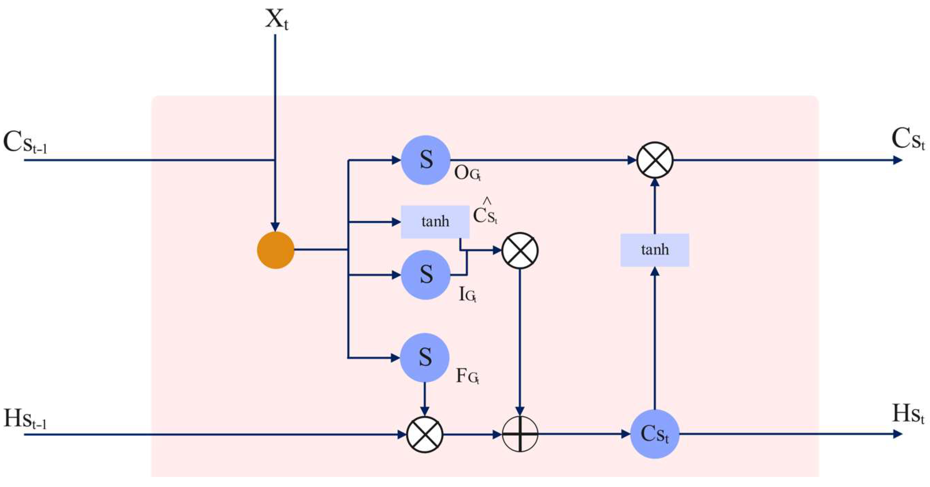
3.2. LSTM (Long Short-Term Memory)

Similar to RNNs, LSTM consists of chain-like modules; however, the design of the LSTM’s recurring modules is more complex. Each module of an LSTM contains a memory block that is repeated. This memory block is specifically designed to retain data for extended durations. Constant error carousel (CEC) cells and three gates, which are specialized multiplicative units, are the four components of the memory block. The gradient remains when an LSTM is trained using backpropagation via time, as the CEC cell propagates in a direction perpendicular to the entire chain in the absence of any activation function. Long short-term model (LSTM) dependencies have been observed to be more proficient than RNNs in this regard due to the unaltered transmission of information via the cells [29].

The three gates depicted in Figure 4 of an LSTM are responsible for the management and adjustment of the hidden state (Hst) and cell state (Cst): the input gate (IGt), the forget gate (FGt), and the output gate (OGt) [7]. These three gates function as filters for various reasons [53]. What information will be removed from the Cs_t is decided by the FG_t, what information will be added to the Cs_t is decided by the IG_t, and the OG_t defines which Cs_t information is used as the output [7]. Each memory block has its own set of input, forget, and output gates that regulate how data move around inside the block. The input gate governs the flow of inputs into the memory cell, whereas the forget gate assesses the condition of the cell’s contents. In contrast, the output gate controls the flow of cell activations [16]. In contrast to conventional RNNs, LSTM cells’ three-gate architecture allows them to effectively capture complicated connections in time series over both the short and long term [52].

These are the transition equations for an LSTM:

$$\mathrm{F}{\mathrm{G}}_{\mathrm{t}}=\mathrm{S}\left({\mathrm{W}}_{\mathrm{F}}\right[\mathrm{H}{\mathrm{s}}_{\mathrm{t}-1},{\mathrm{X}}_{\mathrm{t}}]+{\mathrm{b}}_{\mathrm{F}}),$$

(5)

$$\mathrm{I}{\mathrm{G}}_{\mathrm{t}}=\mathrm{S}\left({\mathrm{W}}_{\mathrm{I}}\right[\mathrm{H}{\mathrm{s}}_{\mathrm{t}-1},{\mathrm{X}}_{\mathrm{t}}]+{\mathrm{b}}_{\mathrm{I}}),$$

(6)

$$\widehat{\mathrm{C}}{\mathrm{s}}_{\mathrm{t}}=\tan \mathrm{h}({\mathrm{W}}_{\mathrm{C}}[\mathrm{H}{\mathrm{s}}_{\mathrm{t}-1},{\mathrm{X}}_{\mathrm{t}}]+{\mathrm{b}}_{\mathrm{C}}),$$

(7)

$$\mathrm{C}{\mathrm{s}}_{\mathrm{t}}={\mathrm{FG}}_{\mathrm{t}}\odot \mathrm{C}{\mathrm{s}}_{\mathrm{t}-1}+{\mathrm{IG}}_{\mathrm{t}}\odot \widehat{\mathrm{C}}{\mathrm{s}}_{\mathrm{t}},$$

(8)

$$\mathrm{O}{\mathrm{G}}_{\mathrm{t}}=\mathrm{S}\left({\mathrm{W}}_{\mathrm{O}}\right[\mathrm{H}{\mathrm{S}}_{\mathrm{t}-1},{\mathrm{X}}_{\mathrm{t}}]+{\mathrm{b}}_{\mathrm{O}}),$$

(9)

$$\mathrm{H}{\mathrm{s}}_{\mathrm{t}}=\mathrm{O}{\mathrm{G}}_{\mathrm{t}}\odot \tan \mathrm{h}(\mathrm{C}{\mathrm{s}}_{\mathrm{t}}),$$

(10)

where IG_t, OG_t, and FG_t represent input, output, and forget gates; W_I, W_O, W_F, and W_C are weights for each gate; and b_F, b_C, b_O, and b_I stand for the bias terms. The logistic sigmoid function is denoted by S, while the hyperbolic tangent function is represented by tanh. The sign $\odot$ is the scalar product of two vectors; ${\mathrm{C}}_{{\mathrm{s}}_{\mathrm{t}}}$ and $\hat{\mathrm{C}}{\mathrm{s}}_{\mathrm{t}}$ stand for the current and updated cell states, and X_t and ${\mathrm{H}}_{{\mathrm{s}}_{\mathrm{t}}}$ signify the input and output of the cell, respectively.

3.3. Sensitivity Analysis

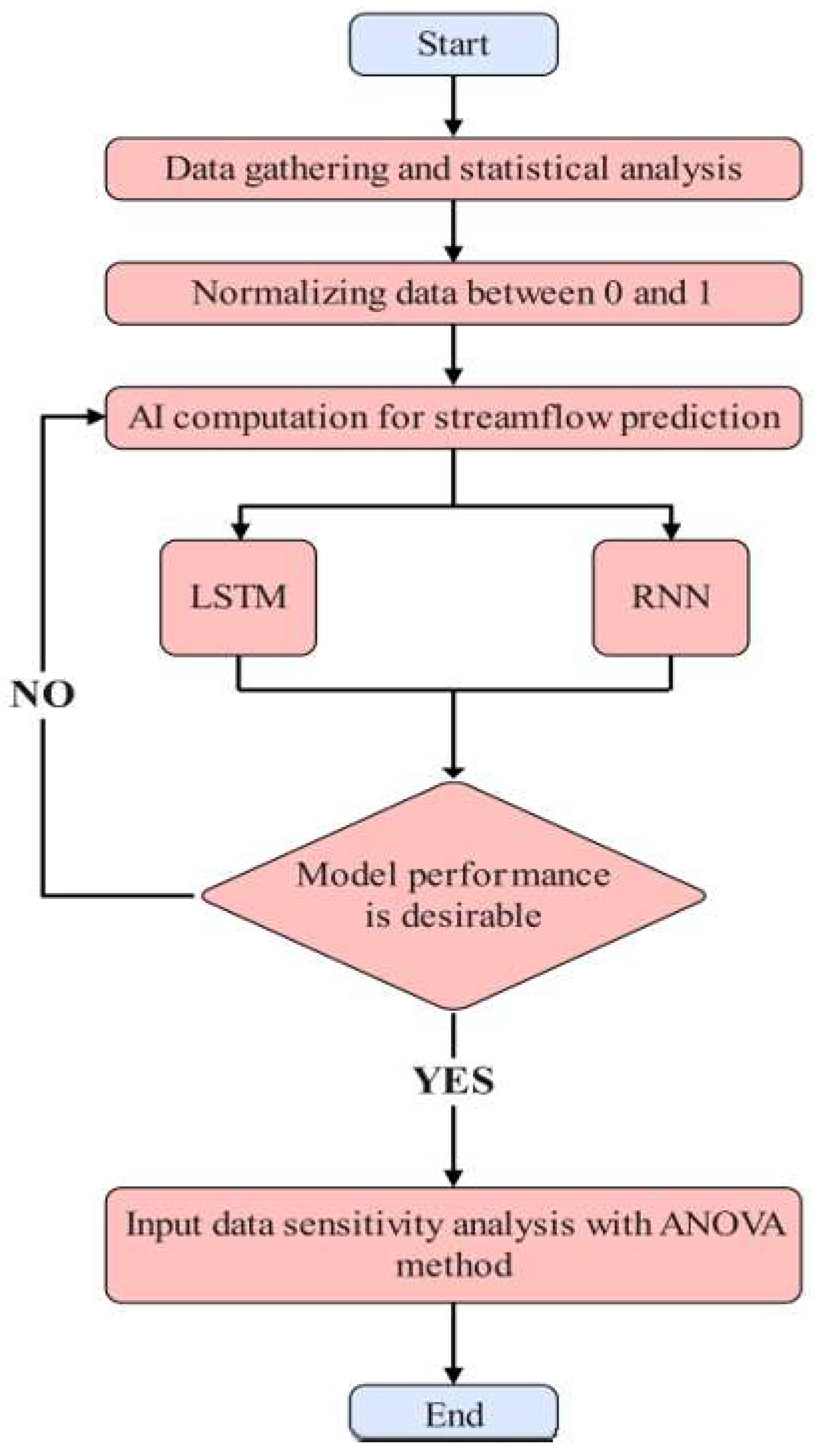
In this study, we used the one-way analysis of variance (ANOVA) calculated by design expert software. The variance value (S2) can be used to figure out the standard deviation (S) using the following formula [54]:

$${\mathrm{S}}^2=\frac{\sum (\mathrm{X}\mathrm{i}-\overline{\mathrm{x}})}{(\mathrm{N}-1)}$$

(11)

With a degree of confidence of 95% and a significance level of 5%, we tested for a significant difference in the X_i variable between two stations. The p-value was used as an indicator of the significance of the X_i variable difference between stations. If the p-value (sig) is less than 0.05, then there is a significant difference between the two stations with respect to the X_i variable. If the p-value (sig) is larger than 0.05, consequently, disparity is not statistically significant; that is, the X_i variable exhibits no variation among the stations [55].

4. Methodology

4.1. LSTM and RNN Model Development

In Figure 5, the research roadmap for the study is shown graphically. To predict the Zarrine River’s monthly streamflow, LSTM and RNN networks were used. After thorough data collection, a descriptive statistical analysis was produced. As such, the training, validation and testing sample data for the years 1979–1999 (400 data points), 2004–2014, and 1999–2004 (a total of 87 data points) were studied, respectively (117 data points). The testing dataset contains information that was excluded from the training phase in order to assess the effectiveness of the calculative algorithm. In contrast, overfitting is avoided by using the validation dataset to identify the ideal model variables. Due to the absence of established methods for identifying input variables, trial and error is required to determine which input factors have the greatest impact on the model’s output.

To ascertain the model structure that exhibited the maximum performance, a total of five model structures were employed, each with a unique set of input variables and a lag time of up to four months (see

Table 1. The architectures of the LSTM and RNN networks’ models.

Name	Input
Scenario 1 (S1)	$Q_{us}^t; P^t; T_{max}^t; T_{min}^t; T_{avg}^t$
Scenario 2 (S2)	$Q_{us}^t, Q_{us}^{t-1}; Q^{t-1}; P^t, P^{t-1}; T_{max}^t, T_{max}^{t-1}; T_{min}^t, T_{min}^{t-1 }; T_{avg }^t, T_{avg}^{t-1}$
Scenario 3 (S3)	$Q_{us}^t to Q_{us}^{t-2}; Q^{t-1} to Q^{t-2}; P^t to P^{t-2}; T_{max}^t to T_{max}^{t-2}; T_{min}^t to T_{min}^{t-2 }; T_{avg }^t to T_{avg}^{t-2}$
Scenario 4 (S4)	$Q_{us}^t to Q_{us}^{t-3}; Q^{t-1} to Q^{t-3}; P^t to P^{t-3}; T_{max}^t to T_{max}^{t-3}; T_{min}^t to T_{min}^{t-3}; T_{avg }^t to T_{avg}^{t-3}$
Scenario 5 (S5)	$Q_{us}^t to Q_{us}^{t-4}; Q^{t-1} to Q^{t-4}; P^t to P^{t-4}; T_{max}^t to T_{max}^{t-4}; T_{min}^t to T_{min}^{t-4}; T_{avg }^t to T_{avg}^{t-4}$

). In Table 1, ${\mathrm{Q}}^{\mathrm{t}}$ and ${\mathrm{Q}}_{\mathrm{u}\mathrm{s}}^{\mathrm{t}}$ represent the current and upstream station streamflows at month t, respectively. P^t represents precipitation at month t. ${\mathrm{T}}_{\mathrm{m}\mathrm{a}\mathrm{x}}^{\mathrm{t}},{\mathrm{T}}_{\mathrm{m}\mathrm{i}\mathrm{n}}^{\mathrm{t}},\mathrm{a}\mathrm{n}\mathrm{d}{\mathrm{T}}_{\mathrm{a}\mathrm{v}\mathrm{g}}^{\mathrm{t}}$ are three variant temperatures in the month. The model’s structure is shown by t₁, t₂, t₃, and t₄ with a delay of one to four months between each event. Scenario 3, 4, and 5 incorporate all input parameters with two to four-month latency. However, scenarios 1 and 2 have zero and one-month lag time and include all features except the current station’s streamflow. The first station in scenario 1 does not incorporate upstream station streamflow (Safakhaneh station). Setting hype-parameters for the LSTM and RNN networks is next. Adjusting hype accurate predictions requires careful network hype-parameter adjustment. Kan et al. in [11] used the trial–error method to obtain the hype-parameters with the best validation dataset model performance. Thus, many experiments are run with a large parameter range.

Given the utilization of the stochastic gradient descent optimization technique during the training phase of deep learning networks, a cost function was devised to iteratively assess the model’s condition. Following that, adjustments were made to the network’s weights with the intention of enhancing the model’s performance in the forthcoming evaluation. The loss function in the present study is denoted by the mean squared error (MSE) (Equation (12)).

$$\mathrm{MSE}={\sum }_{\mathrm{t}-1}^{\mathrm{n}}{({\mathrm{Q}}_{{\mathrm{o}}_{\mathrm{t}}}-{\mathrm{Q}}_{{\mathrm{p}}_{\mathrm{t}}})}^2$$

(12)

where ${\mathrm{Q}}_{{\mathrm{o}}_{\mathrm{t}}}$ and ${\mathrm{Q}}_{{\mathrm{p}}_{\mathrm{t}}}$ represent the streamflow as observed and projected at time t, respectively.

Finally, the third step was to utilize the ANOVA method in order to evaluate the sensitivity analysis of input data.

4.2. Data Normalization

The pre-processing phase of raw data normalization is a key step in training machine learning methods. By standardizing the attribute data to a single scale, one can circumvent numerical obstacles presented by the model, thereby facilitating a more efficient and precise modeling process. For machine learning approaches in general and ANN networks in particular, Ref. [56] advised incorporating data normalization into the range [0,1]. To achieve data normalization for the purposes of this study, the subsequent equation is utilized.

$${\mathrm{I}}_{\mathrm{n}}=\frac{{\mathrm{I}}^{\mathrm{*}}-{\mathrm{I}}_{\mathrm{m}\mathrm{a}\mathrm{x}}}{{\mathrm{I}}_{\mathrm{m}\mathrm{a}\mathrm{x}}-{\mathrm{I}}_{\mathrm{m}\mathrm{i}\mathrm{n}}}$$

(13)

where I_max, I_min, I_n, and I* represent, respectively, the maximum and minimum values, and the raw dataset and the normalized data.

4.3. The Criteria of Model Evaluation

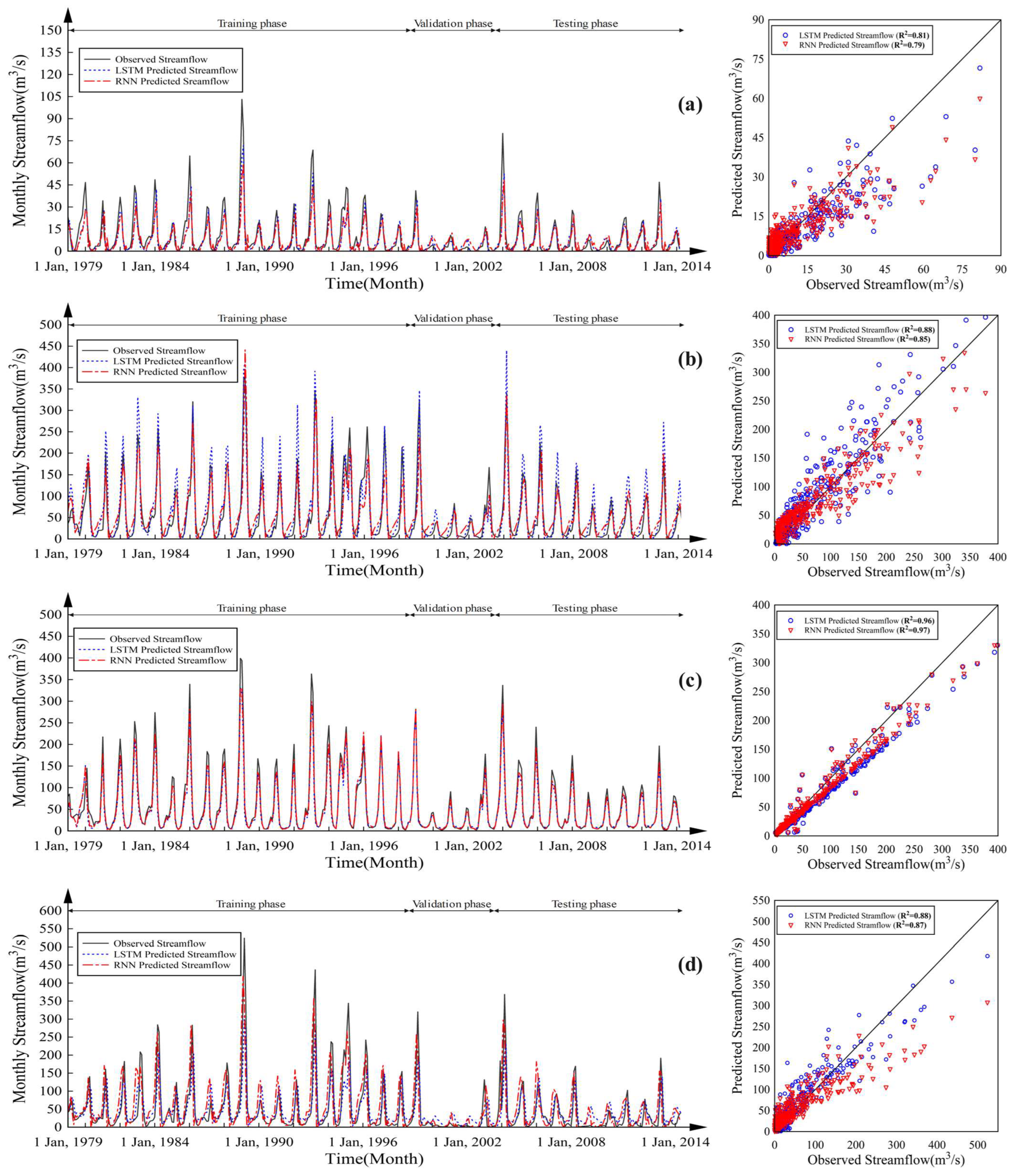
An evaluation of the precision and dependability of streamflow forecasting was performed utilizing three distinct statistical metrics: the Nash Sutcliffe coefficient (NSE), the coefficient of determination (R²), and the root mean square error (RMSE). Equation (14) represents the Sutcliffe Nash coefficient (NSE), a widely employed and reliable metric utilized in the evaluation of hydrological model performance. It signifies the proportion between the variances in observed and projected data. NSE ratings exhibit a range between 0 and 1, where values approaching 1 indicate enhanced performance [57]. The linear link between the data that were seen and the data that were anticipated is represented by the coefficient of determination (R²), which is found in Equation (15) and has a range of [0,1]. When the value of R² is closer to 1, the prediction model generates outcomes that are more accurate. An expression representing the magnitude of the deviation between actual and expected values is known as the root mean square error (RMSE) (Equation (16)). If the value of RMSE is near zero, the forecast is very precise.

$$\mathrm{N}\mathrm{S}\mathrm{E}=1-\frac{{\sum _{\mathrm{t}=1}({\mathrm{Q}}_{\mathrm{p}}-{\mathrm{Q}}_{\mathrm{o}})}^2}{{\sum _{\mathrm{t}=1}({\mathrm{Q}}_{\mathrm{o}}-\overline{\mathrm{Q}})}^2}$$

(14)

$${\mathrm{R}}^2=1-\frac{{\sum ({\mathrm{Q}}_{\mathrm{p}}-{\mathrm{Q}}_{\mathrm{o}})}^2}{\sum {\mathrm{Q}}_{\mathrm{p}}^2}$$

(15)

$$\mathrm{R}\mathrm{M}\mathrm{S}\mathrm{E}=\sqrt{\frac{{\sum ({\mathrm{Q}}_{\mathrm{p}}-{\mathrm{Q}}_{\mathrm{o}})}^2}{\mathrm{N}}}$$

(16)

where $\overline{{\mathrm{Q}}_{}}$, Q_p, and Q_o, indicate the average, predicted, and observed values, respectively, whereas N denotes the quantity of data points.

5. Results

5.1. Evaluation of LSTM and RNN Networks

As stated earlier, the research utilized LSTM and RNN networks with five unique model architectures in order to forecast streamflow at consecutive hydrometric stations located in the Zarrine River basin. In order to reduce the potential for overfitting, a train–validation–test methodology was implemented. The model was trained using the training dataset, while the validation dataset was employed to determine the most effective model structure and its corresponding parameters. Following that, the selected model was assessed using an unobserved test dataset. The level of generalization error of the model was ascertained through a comparison between the evaluation of the test and validation sets’ performance. When the outcomes of the two sets exhibited comparability, it indicated that the model possessed a minimal generalization error and had not been overfit.

The results of the LSTM and RNN models for the four hydrometric stations and five structures specified in Table 1 are presented in

Table 2. A comparison of the performance of LSTM and RNN-based streamflow forecasting models with varied monthly lag times for four station structures in the Zarrine River basin.

			Training Phase			Validation Phase			Testing Phase
Station	Model Type	Structure	NSE	R2	RMSE	NSE	R2	RMSE	NSE	R2	RMSE
Safakhaneh (#1)	LSTM	S1	0.21	0.42	13.3	0.44	0.31	3.4	0.01	0.3	11.8
		S2	0.48	0.65	10.8	0.38	0.21	5.7	0.44	0.48	8.9
		S3	0.77	0.83	7.17	0.53	0.24	4.2	0.64	0.67	7.2
		S4	0.56	0.63	10	0.58	0.27	3.7	0.55	0.58	8.0
		S5	0.68	0.77	8.4	0.68	0.71	5.0	0.7	0.73	6.3
	RNN	S1	0.56	0.7	17.21	0.44	0.35	3.3	0.58	0.04	14.6
		S2	0.62	0.16	15.1	0.68	0.1	3.3	0.61	0.1	11.9
		S3	0.68	0.75	8.4	0.65	0.5	2.5	0.64	0.67	7.1
		S4	0.69	0.75	8.3	0.64	0.56	2.5	0.68	0.71	6.7
		S5	0.75	0.81	7.5	0.75	0.76	5.0	0.76	0.79	5.6
Bookan reservoir (#2)	LSTM	S1	0.82	0.12	169	0.54	0.2	79	0.76	0.08	160
		S2	0.79	0.85	35.3	0.63	0.00	50.4	0.81	0.89	24.1
		S3	0.84	0.88	30.5	0.59	0.62	20.7	0.73	0.88	28.8
		S4	0.77	0.79	37	0.51	0.59	23.7	0.77	0.78	26.6
		S5	0.79	0.81	35.2	0.73	0.58	42.3	0.79	0.81	24.4
	RNN	S1	0.77	0.01	165.1	0.58	0.01	68.8	0.87	0.2	137.5
		S2	0.83	0.86	32.1	0.73	0.69	19.5	0.82	0.88	23.8
		S3	0.84	0.84	31.3	0.84	0.7	19.3	0.86	0.87	20.6
		S4	0.81	0.82	34.1	0.69	0.73	18.8	0.84	0.84	22.3
		S5	0.77	0.83	37.5	0.77	0.8	21.4	0.82	0.85	22.7
Qezkorpi (#3)	LSTM	S1	0.96	0.96	14.5	0.98	0.98	4.8	0.96	0.98	11
		S2	0.93	0.96	20.6	0.94	0.99	8.2	0.93	0.99	15
		S3	0.93	0.96	19	0.92	0.98	9.3	0.94	0.98	25.2
		S4	0.78	0.8	35.8	0.6	0.65	22.6	0.81	0.82	25.25
		S5	0.93	0.96	20.1	0.95	0.99	9.8	0.93	0.99	13.8
	RNN	S1	0.96	0.96	15.1	0.9	0.98	10.4	0.97	0.99	9.6
		S2	0.95	0.96	16.3	0.97	0.98	5.4	0.99	0.99	5.6
		S3	0.97	0.95	81.2	0.93	0.91	35.6	0.93	0.97	59.5
		S4	0.9	0.96	89.1	0.91	0.98	40.26	0.96	0.99	64.9
		S5	0.95	0.97	16.7	0.96	0.99	8.5	0.96	0.66	10.8
Nezamabad (#4)	LSTM	S1	0.65	0.01	16.7	0.28	0.53	3.3	0.57	0.01	13.8
		S2	0.59	0.64	9.6	0.56	0.28	4.9	0.51	0.51	8.3
		S3	0.78	0.82	7.03	0.48	0.04	3.4	0.61	0.64	7.4
		S4	0.57	0.63	9.8	0.51	0.31	3.6	0.56	0.58	7.9
		S5	0.48	0.11	10.8	0.66	0.11	6.76	0.47	0.52	8.5
	RNN	S1	0.65	0.78	47.8	0.55	6.2	14.5	0.64	0.75	31
		S2	0.81	0.84	35	0.65	0.69	12.7	0.79	0.79	23.6
		S3	0.87	0.88	28.7	0.65	0.76	12.8	0.78	0.83	24.1
		S4	0.88	0.89	26.9	0.73	0.79	11.7	0.8	0.84	22.8
		S5	0.82	0.29	101.3	0.77	0.31	36.5	0.75	0.2	61.1

. In order to prevent model overfitting, the selection of the ideal structure is based on which one achieves the highest performance measures, namely, NSE and R², while ensuring that the outcomes of the validation and test phases stay comparable.

As presented in Table 2, there is a significant enhancement in the performance of the models at the initial station, Safakhaneh, when transitioning from the S1 to S5 structure. This improvement suggests that utilizing antecedent data leads to the best output results. Notably, during the testing phase, the RNN model consistently outperforms the LSTM network for Safakhaneh, exhibiting higher values for NSE (0.76) and R² (0.79) and a lower RMSE (5.6). While the model structures for Safakhaneh do not incorporate upstream station streamflow data, downstream stations benefit from it. The RNN model’s output for the S5 structure in Safakhaneh station serves as upstream streamflow input for predicting outflow in the Bookan reservoir model. The RNN model consistently outperforms the LSTM model across all model structures. The S3 model, which includes all input variable values and has a delay of four months, demonstrates particularly outstanding results in this regard. Within this context, the accuracy measures are as follows: RMSE (22.8), R² (0.84), and NSE (0.8). This indicates that the performance of the model has a tendency to decrease when excessive inputs are introduced, which highlights the significance of maintaining a balanced level of model complexity.

In light of the downstream location of the Qezkorpi station in relation to the Bookan reservoir, the models utilize the reservoir’s monthly discharge as the upstream outflow input. Each of the model structures exhibits robust performance and produces similar outcomes. On the contrary, the RNN model that incorporates the S2 structure, which includes all input variables, and incorporates a lag period of one month demonstrates a marginal improvement in accuracy. The assessment criteria for the S2 model include NSE, R², and RMSE values of 0.99, 0.99, and 5.6, respectively, which indicate its exceptional accuracy. An outlet station of utmost importance in the Zarrine River basin is Nezamabad, which is tasked with feeding Lake Urmia with outflow. With the exception of S1, the RNN network demonstrates favorable output results across a range of structures. The S4 structure exhibits the most remarkable model performance, as seen by its NSE, R², and RMSE values of 0.8, 0.84, and 22.8, respectively. The outcomes underscore the remarkable capability of the RNN network to forecast monthly streamflow at consecutive stations across the basin, with a particular emphasis on the outlet station that aids in the inflow of Lake Urmia.

This study utilizes a successive station procedure to simulate the streamflow at each station. Therefore, the models use the downstream simulated streamflow in their structure, leading to improved prediction results at each station. The Boukan reservoir uses the Safakhaneh station’s streamflow, which is located on the river tributary leading to the reservoir. Thus, the simulated results improved at each upstream station. However, the model performance in the Nezamabad station (outlet station) is decreased due to the presence of numerous tributaries between the Qezkorpi station and the outlet station. This will increase the uncertainty in the model and reduce the model performance.

The scatter plots show the observed and predicted hydrographs for the highest performing models during the validation, training, and testing phases, and each hydrometric station is depicted in Figure 6. Streamflow fluctuations are predicted with a higher degree of accuracy by the RNN model, as evidenced by the hydrographs. Furthermore, the scatter plots reveal that in each station, the RNN model demonstrates higher R² values for streamflow compared to the LSTM model. Although the model displays certain incongruities, namely, during periods of high flow at the Safakhaneh station and Bookan reservoir, its operational efficacy remains satisfactory when applied to flows in the low to medium range. Significantly, the RNN model exhibits constant excellence across all flow circumstances for the stations of Qezkorpi and Nezamabad. The findings underscore the model’s enhanced performance for stations situated downstream as opposed to those situated upstream, a pattern that corresponds well with the calibrated river flow successfully reaching downstream stations. In general, these techniques have the potential to be examined and applied across various scientific disciplines, with particular relevance to environmental studies [58,59,60,61].

However, it is crucial to acknowledge that despite the high accuracy of the model, inherent uncertainties and complexities in flood dynamics pose significant challenges to comprehensive hazard management. One of the fundamental scientific aspects contributing to potential errors lies in the stochastic nature of the phenomenon. Flood events are influenced by a myriad of random variables, such as precipitation patterns, soil moisture content, topography, and human activities, making it challenging to predict with absolute certainty [62]. Moreover, the dynamic nature of hydrological processes introduces an additional layer of complexity. River basins are intricate systems characterized by nonlinear interactions between various components, including rainfall, runoff, infiltration, and channel flow. The interplay of these factors can lead to emergent behaviors that are difficult to capture accurately in a predictive model. As a result, the model’s susceptibility to errors increases, especially during extreme or unprecedented events that may deviate from historical patterns [63]. Another scientific consideration is the impact of climate change on flood dynamics. Climate variability introduces new challenges in predicting future flood scenarios, as shifts in precipitation patterns, temperature, and sea level contribute to altering the hydrological cycle. The model’s reliance on historical data may not adequately account for these evolving climatic conditions, leading to potential inaccuracies in long-term predictions [64]. Furthermore, uncertainties in data quality and availability can significantly affect the model’s performance. Incomplete or inaccurate data, especially in regions with limited monitoring infrastructure, may compromise the model’s ability to provide reliable flood forecasts. It is essential to continually update and validate the model with the latest data to enhance its robustness and reliability in real-world applications [65].

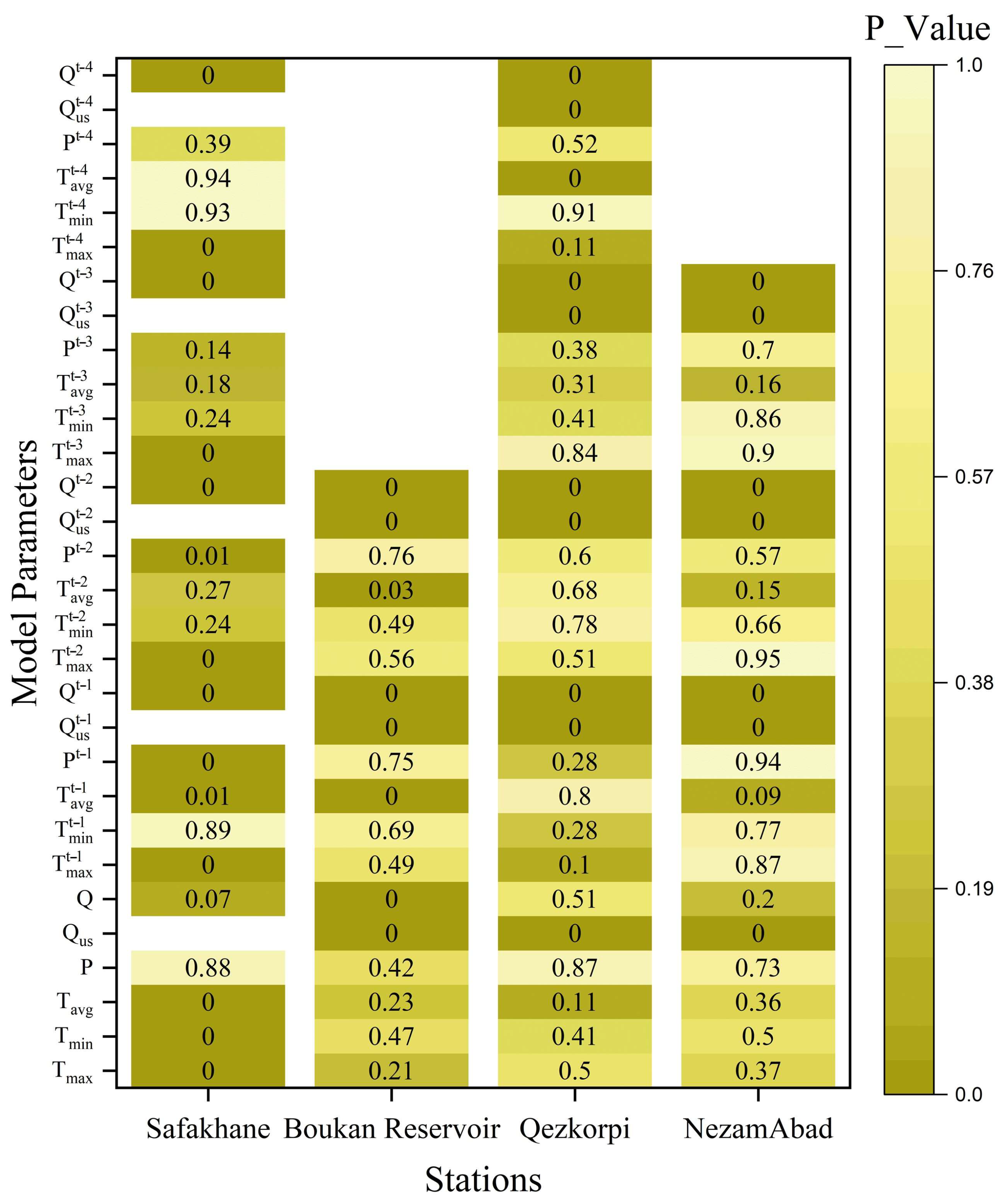
5.2. Sensitivity Analysis

Conducting a one-way analysis of variance (ANOVA) sensitivity study is critical for determining how different input parameters affect the performance of a model. A critical statistical indicator, the p-value acquired by a one-way ANOVA sensitivity analysis, measures the significance of the observed discrepancies in the model’s output that may be ascribed to various input parameters. A p-value that is small, usually less than a pre-established significance level (e.g., 0.05), provides robust support for rejecting the null hypothesis. This implies that at least one of the input parameters significantly influences the output of the model. On the contrary, a substantial p-value indicates that the available evidence is inadequate to reject the null hypothesis, thus suggesting that the input parameters might not significantly influence the operational efficiency of the model. ANOVA goes beyond merely identifying influential factors; it provides a statistical basis for comparing their individual contributions. This comprehensive analysis aids in discerning not only which factors play a significant role but also the extent to which they affect the accuracy of our streamflow predictions. The utilization of ANOVA in our sensitivity analysis strengthens the scientific rigor of our approach, allowing us to pinpoint and prioritize the key factors influencing the performance of our models.

The outcomes of the sensitivity analysis, as determined using one-way ANOVA, are depicted in Figure 7. In contrast to precipitation and minimum and average temperature, which have the least impact on the model’s output, the results indicate that upstream station streamflow, station streamflow, and maximum temperature exert the greatest influence on the model’s output. The downstream streamflow is not included in the sensitivity analysis of the Safakhaneh station; thus, the analysis only shows a great impact on the maximum temperature and the antecedent streamflow of that station. The other three stations not only show high influence on those inputs but also the downstream station of each one of the stations.

6. Physical Mechanism Analysis

The Muskingum–Cunge method is a widely used technique for predicting the flow of water through river channels, particularly in hydrological modeling. This method is essentially a routing equation that helps simulate the movement of water through a basin over time (Equation (17)).

Q_out (t) = K⋅Δt⋅(dQ_in(t)/dt) + (1−K)⋅Q_in(t−Δt)

(17)

where Q_out (t) is the outflow at time t; Q_in (t) is the inflow at time t; Δt is the time step; and K is the routing parameter.

This method essentially calculates the outflow at a given time (Q_out (t)) based on the inflow at the same time (Q_in(t)) and the inflow at a previous time (Q_in(t − Δt)), along with a fraction (K) of the rate of change in inflow with respect to time [66,67].

In the present research, the physical assessment of flow in the basin is programmed as per MATLAB 2021b software. The outcomes are demonstrated in Figure 8. In the model, as per the statistical data of the Water Management Organization of Iran, at the evaluated time, the maximum, average, and minimum flows of the Zarrine River basin are considered equal to 560, 250, and 60 m³/s, respectively. Also, the total time and Δt are adjusted to 100 and 30, respectively. In the model, different K values from 0 to 1 are computed in the present model. By concentrating on Figure 8, it can be concluded that the physical state of the basin is computed from 60 to 350 in the time steps, which is seen as the average of different station flows in Figure 6. Therefore, the physical analysis of average stations in the basin is close to the absolute measured values at different stations. Finally, the physical analysis of the basin approves the machine learning outputs of this study as well as the real data of the case study. In general, the contour plot provides a comprehensive visual representation of the dynamics of the outflow, considering the interplay between time and the parameter K in the Muskingum–Cunge method. It helps users understand how adjustments in the parameter K impact the outflow at different time points during the simulation.

7. Conclusions

In this study, we established a robust forecasting framework and evaluated the predictive capabilities of two prominent networks, namely, ANN and LSTM models, applied to monthly streamflow forecasting. The focus on the Zarrine River basin, a significant sub-basin of Lake Urmia, allowed us to attribute a substantial portion of variations in the lake’s water level to the dynamic streamflow of the Zarrine River. Our models, supported by an effective application of the ANOVA method, demonstrated remarkable performance in discerning the relative relevance of input factors. Examining streamflow at the current and upstream stations, precipitation, and temperature variables provided valuable insights. Crucially, our findings underscored the superiority of the RNN model over LSTM in accurately mimicking the rainfall–runoff processes inherent in monthly streamflow forecasting. The RNN’s capacity to filter out redundant information during the modeling of rainfall–runoff connections contributed to its superior performance, contrasting with the discernible decline in the accuracy of the typical ANN model. In terms of sensitivity analysis, the one-way ANOVA approach highlighted that maximum temperature, station streamflow, and upstream station streamflow significantly influenced the RNN model’s output. This insight emphasizes the critical role of these factors in shaping the predictive accuracy of our model.

Connecting these results with our study objectives, we aimed to provide not only a comparative evaluation of ANN and LSTM models but also a nuanced understanding of the factors influencing streamflow predictions. Looking ahead, these findings have broader implications for hydrological research and practical applications. They suggest the potential of RNN networks, particularly in mitigating information redundancy, and emphasize the importance of considering key factors like temperature and upstream streamflow in hydrological modeling. This study contributes to advancing our understanding of effective methodologies for streamflow forecasting, paving the way for future research and informed water resource management practices.

References

1. Feng, Z.; Niu, W.; Tang, Z.; Jiang, Z.; Xu, Y.; Liu, Y.; Zhang, H. Monthly Runoff Time Series Prediction by Variational Mode Decomposition and Support Vector Machine Based on Quantum-Behaved Particle Swarm Optimization. J. Hydrol. 2020, 583, 124627. [Google Scholar] [CrossRef]
2. Nohara, D.; Nishioka, Y.; Hori, T.; Sato, Y. Real-Time Reservoir Operation for Flood Management Considering Ensemble Streamflow Prediction and Its Uncertainty. In Advances in Hydroinformatics; Springer: Berlin/Heidelberg, Germany, 2016; pp. 333–347. [Google Scholar]
3. Sabzi, H.Z.; King, J.P.; Abudu, S. Developing an Intelligent Expert System for Streamflow Prediction, Integrated in a Dynamic Decision Support System for Managing Multiple Reservoirs: A Case Study. Expert Syst. Appl. 2017, 83, 145–163. [Google Scholar] [CrossRef]
4. Young, C.-C.; Liu, W.-C. Prediction and Modelling of Rainfall–Runoff during Typhoon Events Using a Physically-Based and Artificial Neural Network Hybrid Model. Hydrol. Sci. J. 2015, 60, 2102–2116. [Google Scholar] [CrossRef]
5. Partington, D.; Brunner, P.; Simmons, C.T.; Werner, A.D.; Therrien, R.; Maier, H.R.; Dandy, G.C. Evaluation of Outputs from Automated Baseflow Separation Methods against Simulated Baseflow from a Physically Based, Surface Water-Groundwater Flow Model. J. Hydrol. 2012, 458, 28–39. [Google Scholar] [CrossRef]
6. Zhang, J.; Chen, X.; Khan, A.; Zhang, Y.; Kuang, X.; Liang, X.; Taccari, M.L.; Nuttall, J. Daily Runoff Forecasting by Deep Recursive Neural Network. J. Hydrol. 2021, 596, 126067. [Google Scholar] [CrossRef]
7. Gao, S.; Huang, Y.; Zhang, S.; Han, J.; Wang, G.; Zhang, M.; Lin, Q. Short-Term Runoff Prediction with GRU and LSTM Networks without Requiring Time Step Optimization during Sample Generation. J. Hydrol. 2020, 589, 125188. [Google Scholar] [CrossRef]
8. Pulukuri, S.; Keesara, V.R.; Deva, P. Flow Forecasting in a Watershed Using Autoregressive Updating Model. Water Resour. Manag. 2018, 32, 2701–2716. [Google Scholar] [CrossRef]
9. Rath, A.; Samantaray, S.; Bhoi, K.S.; Swain, P.C. Flow Forecasting of Hirakud Reservoir with ARIMA Model. In Proceedings of the IEEE 2017 International Conference on Energy, Communication, Data Analytics and Soft Computing (ICECDS), Chennai, India, 1–2 August 2017; pp. 2952–2960. [Google Scholar]
10. Zhang, J.; Xiao, H.; Fang, H. Component-Based Reconstruction Prediction of Runoff at Multi-Time Scales in the Source Area of the Yellow River Based on the ARMA Model. Water Resour. Manag. 2022, 36, 433–448. [Google Scholar] [CrossRef]
11. Kan, G.; Yao, C.; Li, Q.; Li, Z.; Yu, Z.; Liu, Z.; Ding, L.; He, X.; Liang, K. Improving Event-Based Rainfall-Runoff Simulation Using an Ensemble Artificial Neural Network Based Hybrid Data-Driven Model. Stoch. Environ. Res. Risk Assess. 2015, 29, 1345–1370. [Google Scholar] [CrossRef]
12. Gheibi, M.; Moezzi, R. A Social-Based Decision Support System for Flood Damage Risk Reduction in European Smart Cities. Quanta Res. 2023, 1, 27–33. [Google Scholar] [CrossRef]
13. Poonia, V.; Tiwari, H.L. Rainfall-Runoff Modeling for the Hoshangabad Basin of Narmada River Using Artificial Neural Network. Arab. J. Geosci. 2020, 13, 944. [Google Scholar] [CrossRef]
14. Wang, W.; Xu, D.; Chau, K.; Chen, S. Improved Annual Rainfall-Runoff Forecasting Using PSO–SVM Model Based on EEMD. J. Hydroinform. 2013, 15, 1377–1390. [Google Scholar] [CrossRef]
15. Wu, Y.; Wang, Q.; Li, G.; Li, J. Data-Driven Runoff Forecasting for Minjiang River: A Case Study. Water Supply 2020, 20, 2284–2295. [Google Scholar] [CrossRef]
16. Cheng, M.; Fang, F.; Kinouchi, T.; Navon, I.M.; Pain, C.C. Long Lead-Time Daily and Monthly Streamflow Forecasting Using Machine Learning Methods. J. Hydrol. 2020, 590, 125376. [Google Scholar] [CrossRef]
17. Nourani, V.; Komasi, M. A Geomorphology-Based ANFIS Model for Multi-Station Modeling of Rainfall–Runoff Process. J. Hydrol. 2013, 490, 41–55. [Google Scholar] [CrossRef]
18. Alvisi, S.; Franchini, M. Fuzzy Neural Networks for Water Level and Discharge Forecasting with Uncertainty. Environ. Model. Softw. 2011, 26, 523–537. [Google Scholar] [CrossRef]
19. Shortridge, J.E.; Guikema, S.D.; Zaitchik, B.F. Machine Learning Methods for Empirical Streamflow Simulation: A Comparison of Model Accuracy, Interpretability, and Uncertainty in Seasonal Watersheds. Hydrol. Earth Syst. Sci. 2016, 20, 2611–2628. [Google Scholar] [CrossRef]
20. Kalra, A.; Ahmad, S.; Nayak, A. Increasing Streamflow Forecast Lead Time for Snowmelt-Driven Catchment Based on Large-Scale Climate Patterns. Adv. Water Resour. 2013, 53, 150–162. [Google Scholar] [CrossRef]
21. Yu, P.-S.; Yang, T.-C.; Chen, S.-Y.; Kuo, C.-M.; Tseng, H.-W. Comparison of Random Forests and Support Vector Machine for Real-Time Radar-Derived Rainfall Forecasting. J. Hydrol. 2017, 552, 92–104. [Google Scholar] [CrossRef]
22. Mosavi, A.; Ozturk, P.; Chau, K. Flood Prediction Using Machine Learning Models: Literature Review. Water 2018, 10, 1536. [Google Scholar] [CrossRef]
23. Reichstein, M.; Camps-Valls, G.; Stevens, B.; Jung, M.; Denzler, J.; Carvalhais, N. Deep Learning and Process Understanding for Data-Driven Earth System Science. Nature 2019, 566, 195–204. [Google Scholar] [CrossRef] [PubMed]
24. Xiang, Z.; Demir, I. Distributed Long-Term Hourly Streamflow Predictions Using Deep Learning–A Case Study for State of Iowa. Environ. Model. Softw. 2020, 131, 104761. [Google Scholar] [CrossRef]
25. Rangapuram, S.S.; Seeger, M.W.; Gasthaus, J.; Stella, L.; Wang, B.; Januschowski, T. Deep State Space Models for Time Series Forecasting. In Proceedings of the Advances in Neural Information Processing Systems 31: 32nd Conference on Neural Information Processing Systems (NeurIPS 2018), Montréal, QC, Canada, 3–8 December 2018. [Google Scholar]
26. Hochreiter, S.; Schmidhuber, J. Long Short-Term Memory. Neural Comput. 1997, 9, 1735–1780. [Google Scholar] [CrossRef] [PubMed]
27. Mouatadid, S.; Adamowski, J.F.; Tiwari, M.K.; Quilty, J.M. Coupling the Maximum Overlap Discrete Wavelet Transform and Long Short-Term Memory Networks for Irrigation Flow Forecasting. Agric. Water Manag. 2019, 219, 72–85. [Google Scholar] [CrossRef]
28. Zhang, D.; Lindholm, G.; Ratnaweera, H. Use Long Short-Term Memory to Enhance Internet of Things for Combined Sewer Overflow Monitoring. J. Hydrol. 2018, 556, 409–418. [Google Scholar] [CrossRef]
29. Zhang, J.; Zhu, Y.; Zhang, X.; Ye, M.; Yang, J. Developing a Long Short-Term Memory (LSTM) Based Model for Predicting Water Table Depth in Agricultural Areas. J. Hydrol. 2018, 561, 918–929. [Google Scholar] [CrossRef]
30. Wang, Q.; Huang, J.; Liu, R.; Men, C.; Guo, L.; Miao, Y.; Jiao, L.; Wang, Y.; Shoaib, M.; Xia, X. Sequence-Based Statistical Downscaling and Its Application to Hydrologic Simulations Based on Machine Learning and Big Data. J. Hydrol. 2020, 586, 124875. [Google Scholar] [CrossRef]
31. Li, X.; Song, G.; Zhou, S.; Yan, Y.; Du, Z. Rainfall Runoff Prediction via a Hybrid Model of Neighbourhood Rough Set with LSTM. Int. J. Embed. Syst. 2020, 13, 405–413. [Google Scholar] [CrossRef]
32. Ren, Y.; Zeng, S.; Liu, J.; Tang, Z.; Hua, X.; Li, Z.; Song, J.; Xia, J. Mid-to Long-Term Runoff Prediction Based on Deep Learning at Different Time Scales in the Upper Yangtze River Basin. Water 2022, 14, 1692. [Google Scholar] [CrossRef]
33. Zanjanian, H.; Niksokhan, M.H.; Ghorbani, M.; Rezaei, A.R. A Novel Framework for Water Right Conflict Resolution Considering Actors’ Power and Inter-Organizational Relationships Analysis. J. Hydroinform. 2022, 24, 622–641. [Google Scholar] [CrossRef]
34. Zhihua, L.V.; Zuo, J.; Rodriguez, D. Predicting of Runoff Using an Optimized SWAT-ANN: A Case Study. J. Hydrol. Reg. Stud. 2020, 29, 100688. [Google Scholar]
35. Sarzaeim, P.; Bozorg-Haddad, O.; Bozorgi, A.; Loáiciga, H.A. Runoff Projection under Climate Change Conditions with Data-Mining Methods. J. Irrig. Drain. Eng. 2017, 143, 4017026. [Google Scholar] [CrossRef]
36. Asadi, S.; Shahrabi, J.; Abbaszadeh, P.; Tabanmehr, S. A New Hybrid Artificial Neural Networks for Rainfall–Runoff Process Modeling. Neurocomputing 2013, 121, 470–480. [Google Scholar] [CrossRef]
37. Alizadeh, A.; Rajabi, A.; Shabanlou, S.; Yaghoubi, B.; Yosefvand, F. Modeling Long-Term Rainfall-Runoff Time Series through Wavelet-Weighted Regularization Extreme Learning Machine. Earth Sci. Inform. 2021, 14, 1047–1063. [Google Scholar] [CrossRef]
38. Wu, H.; Chen, B. Evaluating Uncertainty Estimates in Distributed Hydrological Modeling for the Wenjing River Watershed in China by GLUE, SUFI-2, and ParaSol Methods. Ecol. Eng. 2015, 76, 110–121. [Google Scholar] [CrossRef]
39. Bae, D.-H.; Trinh, H.L.; Nguyen, H.M. Uncertainty Estimation of the SURR Model Parameters and Input Data for the Imjin River Basin Using the GLUE Method. J. Hydro-Environ. Res. 2018, 20, 52–62. [Google Scholar] [CrossRef]
40. Lee, H.; Balin, D.; Shrestha, R.R.; Rode, M. Streamflow Prediction with Uncertainty Analysis, Weida Catchment, Germany. KSCE J. Civ. Eng. 2010, 14, 413–420. [Google Scholar] [CrossRef]
41. Tang, X.; Zhang, J.; Wang, G.; Jin, J.; Liu, C.; Liu, Y.; He, R.; Bao, Z. Uncertainty Analysis of SWAT Modeling in the Lancang River Basin Using Four Different Algorithms. Water 2021, 13, 341. [Google Scholar] [CrossRef]
42. Zhang, C.; Yan, H.; Takase, K.; Oue, H. Comparison of the Soil Physical Properties and Hydrological Processes in Two Different Forest Type Catchments. Water Resour. 2016, 43, 225. [Google Scholar] [CrossRef]
43. Her, Y.; Yoo, S.-H.; Cho, J.; Hwang, S.; Jeong, J.; Seong, C. Uncertainty in Hydrological Analysis of Climate Change: Multi-Parameter vs. Multi-GCM Ensemble Predictions. Sci. Rep. 2019, 9, 1–22. [Google Scholar] [CrossRef]
44. Zhao, T.; Wang, Q.J.; Bennett, J.C.; Robertson, D.E.; Shao, Q.; Zhao, J. Quantifying Predictive Uncertainty of Streamflow Forecasts Based on a Bayesian Joint Probability Model. J. Hydrol. 2015, 528, 329–340. [Google Scholar] [CrossRef]
45. Liu, Y.; Hou, G.; Huang, F.; Qin, H.; Wang, B.; Yi, L. Directed Graph Deep Neural Network for Multi-Step Daily Streamflow Forecasting. J. Hydrol. 2022, 607, 127515. [Google Scholar] [CrossRef]
46. Najafi, M.R.; Moradkhani, H. Ensemble Combination of Seasonal Streamflow Forecasts. J. Hydrol. Eng. 2016, 21, 4015043. [Google Scholar] [CrossRef]
47. Farajzadeh, J.; Fard, A.F.; Lotfi, S. Modeling of Monthly Rainfall and Runoff of Urmia Lake Basin Using “Feed-Forward Neural Network” and “Time Series Analysis” Model. Water Resour. Ind. 2014, 7, 38–48. [Google Scholar] [CrossRef]
48. Yazdandoost, F.; Moradian, S.; Izadi, A. Evaluation of Water Sustainability under a Changing Climate in Zarrineh River Basin, Iran. Water Resour. Manag. 2020, 34, 4831–4846. [Google Scholar] [CrossRef]
49. Amini, A.; Ghazvinei, P.T.; Javan, M.; Saghafian, B. Evaluating the Impacts of Watershed Management on Runoff Storage and Peak Flow in Gav-Darreh Watershed, Kurdistan, Iran. Arab. J. Geosci. 2014, 7, 3271–3279. [Google Scholar] [CrossRef]
50. Emami, F.; Koch, M. Agricultural Water Productivity-Based Hydro-Economic Modeling for Optimal Crop Pattern and Water Resources Planning in the Zarrine River Basin, Iran, in the Wake of Climate Change. Sustainability 2018, 10, 3953. [Google Scholar] [CrossRef]
51. Graves, A.; Mohamed, A.; Hinton, G. Speech Recognition with Deep Recurrent Neural Networks. In Proceedings of the 2013 IEEE International Conference on Acoustics, Speech and Signal Processing, Vancouver, BC, Canada, 26–31 May 2013; pp. 6645–6649. [Google Scholar]
52. Zhao, Z.; Chen, W.; Wu, X.; Chen, P.C.Y.; Liu, J. LSTM Network: A Deep Learning Approach for Short-term Traffic Forecast. IET Intell. Transp. Syst. 2017, 11, 68–75. [Google Scholar] [CrossRef]
53. Fischer, T.; Krauss, C. Deep Learning with Long Short-Term Memory Networks for Financial Market Predictions. Eur. J. Oper. Res. 2018, 270, 654–669. [Google Scholar] [CrossRef]
54. Johnson, R.A.; Bhattacharyya, G.K. Statistics: Principles and Methods; John Wiley Sons: Hoboken, NJ, USA, 2019; ISBN 1119497116. [Google Scholar]
55. Kaihena, M.; Talakua, C.M.; Pagaya, J.; Talakua, S.M. Analysis of Water Pollution in Microbiology Aspect of Some Watersheds at Ambon City, Maluku Province. In IOP Conference Series: Earth and Environmental Science; IOP Publishing: Bristol, UK, 2021; Volume 805, p. 12021. [Google Scholar]
56. Zhu, S.; Heddam, S.; Nyarko, E.K.; Hadzima-Nyarko, M.; Piccolroaz, S.; Wu, S. Modeling Daily Water Temperature for Rivers: Comparison between Adaptive Neuro-Fuzzy Inference Systems and Artificial Neural Networks Models. Environ. Sci. Pollut. Res. 2019, 26, 402–420. [Google Scholar] [CrossRef]
57. Kumar, P.S.; Praveen, T.V.; Prasad, M.A. Artificial Neural Network Model for Rainfall-Runoff-A Case Study. Int. J. Hybrid Inf. Technol. 2016, 9, 263–272. [Google Scholar] [CrossRef]
58. Gheibi, M.; Chahkandi, B.; Behzadian, K.; Akrami, M.; Moezzi, R. Evaluation of Ceramic Water Filters’ Performance and Analysis of Managerial Insights by SWOT Matrix. Environ. Ind. Lett. 2023, 1, 1–9. [Google Scholar] [CrossRef]
59. Kiyan, A.; Gheibi, M.; Akrami, M.; Moezzi, R.; Behzadian, K. A Comprehensive Platform for Air Pollution Control System Operation in Smart Cities of Developing Countries: A Case Study of Tehran. Environ. Ind. Lett. 2023, 1, 10–27. [Google Scholar] [CrossRef]
60. Kiyan, A.; Gheibi, M.; Akrami, M.; Moezzi, R.; Behzadian, K.; Taghavian, H. The Operation of Urban Water Treatment Plants: A Review of Smart Dashboard Frameworks. Environ. Ind. Lett. 2023, 1, 28–45. [Google Scholar] [CrossRef]
61. Kiyan, A.; Gheibi, M.; Moezzi, R.; Behzadian, K. Smart Dashboard of Water Distribution Network Operation: A Case Study of Tehran. Environ. Ind. Lett. 2023, 1, 46–63. [Google Scholar] [CrossRef]
62. Akbarian, H.; Gheibi, M.; Hajiaghaei-Keshteli, M.; Rahmani, M. A hybrid novel framework for flood disaster risk control in developing countries based on smart prediction systems and prioritized scenarios. J. Environ. Manag. 2022, 312, 114939. [Google Scholar] [CrossRef]
63. Zabihi, O.; Siamaki, M.; Gheibi, M.; Akrami, M.; Hajiaghaei-Keshteli, M. A smart sustainable system for flood damage management with the application of artificial intelligence and multi-criteria decision-making computations. Int. J. Disaster Risk Reduct. 2023, 84, 103470. [Google Scholar] [CrossRef]
64. Nakhaei, M.; Nakhaei, P.; Gheibi, M.; Chahkandi, B.; Wacławek, S.; Behzadian, K.; Chen, A.S.; Campos, L.C. Enhancing community resilience in arid regions: A smart framework for flash flood risk assessment. Ecol. Indic. 2023, 153, 110457. [Google Scholar] [CrossRef]
65. Akrami, M.; Behzadian, K.; Gheibi, M.; Khaleghiabbasabadi, M.; Wacławek, S. Application of Decision-Making Techniques for Prioritizing Water Treatment Technology in Flood Events: A Preventive Crisis Management in the Czech Republic (No. EGU23-9445). In Proceedings of the Copernicus Meetings, Vienna, Austria, 23–28 April 2023. [Google Scholar]
66. Bindas, T.; Tsai, W.P.; Liu, J.; Rahmani, F.; Feng, D.; Bian, Y.; Lawson, K.; Shen, C. Improving large-basin river routing using a differentiable Muskingum-Cunge model and physics-informed machine learning. ESS Open Arch. 2023; Authorea Preprints. [Google Scholar] [CrossRef]
67. Ponce, V.M.; Yevjevich, V. Muskingum-Cunge method with variable parameters. J. Hydraul. Div. 1978, 104, 1663–1667. [Google Scholar] [CrossRef]
Figure 1. Bibliometrix of streamflow prediction subject based on (a) the Sankey diagram and (b) the keyword attributions of streamflow prediction.
Water 16 00208 g001aWater 16 00208 g001b
Figure 2. Study Area Map (A) Iran Map; (B) West Azerbaijan Province Map; (C) Zarrine River Basin Map.
Water 16 00208 g002
Figure 3. Schematic of an RNN cell.
Water 16 00208 g003
Figure 4. Schematic of an LSTM cell.
Water 16 00208 g004
Figure 5. Proposed methodology.
Water 16 00208 g005
Figure 6. The scatter plot and hydrograph of the RNN and LSTM models for the following stations: (a) Nezamabad station; (b) Bookan Reservoir; (c) Ghezkorpi; and (d) Safakhaneh.
Water 16 00208 g006
Figure 7. The results of one-way ANOVA sensitive analysis for various input parameters in the RNN network.
Water 16 00208 g007
Figure 8. The output of basin physical analysis as per Muskingum–Cunge method in this research.
Water 16 00208 g008