Article

Comparison of Machine Learning-Based Predictive Models of the Nutrient Loads Delivered from the Mississippi/Atchafalaya River Basin to the Gulf of Mexico

1
Department of Natural Sciences, Southern University at New Orleans, New Orleans, LA 70126, USA
2
Department of Earth and Environmental Studies, Montclair State University, Montclair, NJ 07043, USA
3
Computational Science Initiative, Brookhaven National Laboratory, Upton, NY 11973, USA
*
Author to whom correspondence should be addressed.
Water 2024, 16(19), 2857; https://doi.org/10.3390/w16192857
Submission received: 8 July 2024 / Revised: 2 October 2024 / Accepted: 6 October 2024 / Published: 8 October 2024

Abstract

:
Predicting nutrient loads is essential to understanding and managing one of the environmental issues faced by the northern Gulf of Mexico hypoxic zone, which poses a severe threat to the Gulf’s healthy ecosystem and economy. The development of hypoxia in the Gulf of Mexico is strongly associated with the eutrophication process initiated by excessive nutrient loads. Due to the complexities in the excessive nutrient loads to the Gulf of Mexico, it is challenging to understand and predict the underlying temporal variation of nutrient loads. The study was aimed at identifying an optimal predictive machine learning model to capture and predict nonlinear behavior of the nutrient loads delivered from the Mississippi/Atchafalaya River Basin (MARB) to the Gulf of Mexico. For this purpose, monthly nutrient loads (N and P) in tons were collected from US Geological Survey (USGS) monitoring station 07373420 from 1980 to 2020. Machine learning models—including autoregressive integrated moving average (ARIMA), gaussian process regression (GPR), single-layer multilayer perceptron (MLP), and a long short-term memory (LSTM) with the single hidden layer—were developed to predict the monthly nutrient loads, and model performances were evaluated by standard assessment metrics—Root Mean Square Error (RMSE) and Correlation Coefficient (R). The residuals of predictive models were examined by the Durbin–Watson statistic. The results showed that MLP and LSTM persistently achieved better accuracy in predicting monthly TN and TP loads compared to GPR and ARIMA. In addition, GPR models achieved slightly better test RMSE score than ARIMA models while their correlation coefficients are much lower than ARIMA models. Moreover, MLP performed slightly better than LSTM in predicting monthly TP loads while LSTM slightly outperformed for TN loads. Furthermore, it was found that the optimizer and number of inputs didn’t show effects on the LSTM performance while they exhibited impacts on MLP outcomes. This study explores the capability of machine learning models to accurately predict nonlinearly fluctuating nutrient loads delivered to the Gulf of Mexico. Further efforts focus on improving the accuracy of forecasting using hybrid models which combine several machine learning models with superior predictive performance for nutrient fluxes throughout the MARB.

1. Introduction

The development of predictive models of nutrient loads may hold the key to understanding and managing the dynamics of hypoxia in the northern Gulf of Mexico. A hypoxic zone (or dead zone) is an area where oxygen levels drop to 2 milligrams per liter or lower and most marine life can no longer survive due to depleted oxygen levels [1]. Hypoxia, which occurs near the coastal Gulf of Mexico, has attracted much attention because it poses a threat to the coastal ecosystem and economy by destroying coastal wetland habitats of numerous fish and wildlife species at an alarming rate [2]. Water quality is deteriorated by increasing municipal and manufacturing needs [2]. Studies shows that the formation of hypoxia in the northern Gulf of Mexico is closely related to excess nutrients (N and P) from the MARB [3]. It is desirable to forecast time series of nutrient loads in order to effectively manage and precisely control excess nutrient export from the MARB. Time series of nutrient load predictions, however, are complex and challenging due to the volatile and nonlinear fluctuations caused by the uncertain sources of nutrient loads relating to changes in the geomorphological nature of riverine and estuarine systems and anthropogenic activities [4,5].
Extensive efforts have been made to pinpoint the critical sources of N and P throughout the MARB, analyze trends of nutrient loads, identify the key influential factors in the nutrient fluxes, investigate the spatial correlations of the distributions of nutrient yields, and assess the effectiveness of nutrient reduction strategies using various statistical approaches [6,7,8,9,10,11,12,13,14,15,16,17,18,19,20,21,22,23]. Simulation techniques, such as SPAtially Referenced Regression On Watershed attributes (SPARROW) models and The Soil and Water Assessment Tool (SWAT), are the most commonly used to describe loads/yields throughout the MARB, analyze the relative importance of various sources, and evaluate the effectiveness of management practices [24,25,26,27]. The ARIMA model has been prevalent in modeling economical and financial time series [28,29,30,31]. The working principle of ARIMA is to investigate the correlations among time series observations and construct a model to describe the structures of the relationships. The patterns in the correlations are assumed stationary over the time and then used to predict the future values. However, the assumption of stationarity poses limitations to the effectiveness of the ARIMA model because, in practice, the time series may be non-stationary [32]. Apart from its restricted assumption, it is hard for the ARIMA model to capture nonlinear variations in time series [32]. The advancement in machine learning architectures brings the possibility of developing sophisticated methods to predict time series with nonlinear behaviors. Time series forecasting problems have been addressed by various machine learning-based approaches. For instance, algorithms of deep learning and random forests have been applied to predict stock time series [33]. Deep learning-based modeling has been reported to under-perform in gradient-boosted trees and random forests and it is difficult to train neural networks. The RNN-based approach is introduced to predict time series of stock returns [34]. RNN-based methods are used in predicting time series in financial markets [34,35]. As a variant of RNN, LSTM is designed to cope with the vanishing gradient situation [36].
In this study, computational frameworks including ARIMA, GPR, MLP, and LSTM were developed to predict monthly nutrient loads (N and P) from 1980 to 2020 and explore the optimal machine learning architecture for the forecasting of time series of nutrient loads. Moreover, to make comparisons to ARIMA and GPR, the neural networks MLP and LSTM are restricted to single hidden layered architectures. The study showed that neural networks LSTM and MLP persistently lead in forecasting competition, as expected, while GPR exhibits comparable performance, better than multi-criteria selected ARIMA. Furthermore, although GPR achieves better accuracy than ARIMA, its R-squared score is the lowest while ARIMA’s is the highest. The article is organized as follows. Section 2 describes the study site, data sources, and the mathematical formalism of ARIMA, GPR, MLP, and LSTM. Section 3 presents descriptive statistics of nutrient loads and predictive performances of ARIMA, GPR, MLP, and LSTM models of nutrient loads. Section 4 discusses the predictive models and concludes the paper.

2. Materials and Methods

Figure 1 shows the flowchart of the methodology, which will be explained in detail in the next subsections.

2.1. Study Site and Data

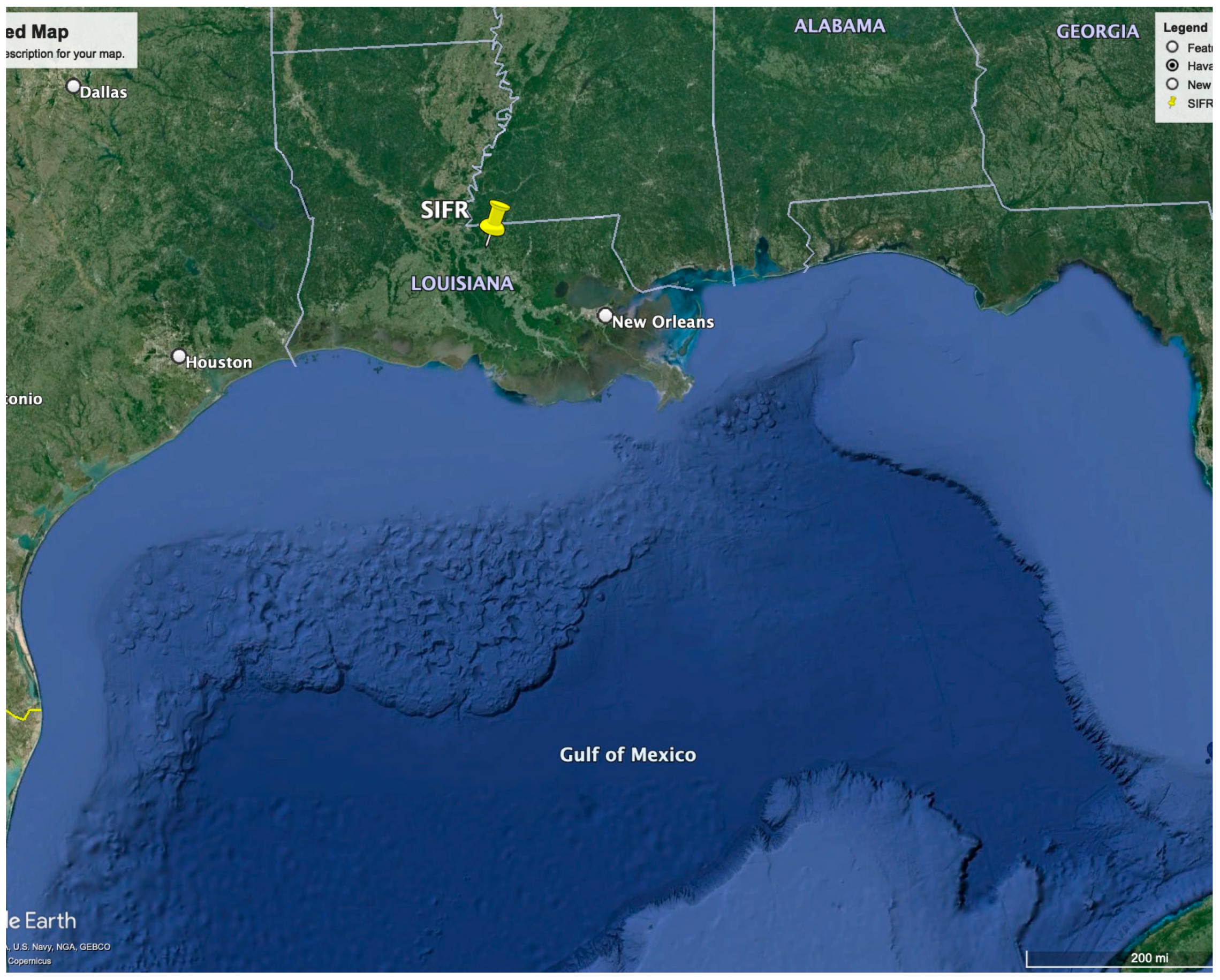
Monthly TN (total nitrogen) and TP (total phosphorus) loads from US Geological Survey (USGS) gaging station 07373420 (Hydrologic unit: 08070100; SITE_ABB: STFR) were downloaded from the government public data source (https://www.sciencebase.gov/catalog/item/61c08ec5d34ee9cd54ed3425; accessed on 20 March 2024). The USGS 07373420 is located on the Mississippi River in West Feliciana Parish, Louisiana in the lower MARB, as shown in Figure 2. The nutrient load data are presented monthly for the period 1980–2020 and are recorded based on the water year (the 12-month period from October 1, for a given year, through 30 September of the following year). The monthly nutrient loads are reported in tons and used for characterization of trends and seasonal variation and development of predictive models.

2.1.1. Data Processing

The dataset used in this study was split into training data (80%) and testing data (20%). The training dataset was used for hyper-parameter tuning. The optimal predictive ARIMA models of the nutrient loads are identified using the software R (version 4.4.0). The analysis on GPR, MLP, and LSTM was carried out in the Python (version 3.10.8) programming environment along with TensorFlow and Keras APIs. The selections of optimal GPR, single-layer MLP, and single-layer LSTM for forecasting nutrient loads were conducted in a Jupyter Notebook (6.5.2). Comparison of performances among predictive models were made.

2.1.2. Assessment Metric

ARIMA, GPR, single layer MLP, and single layer LSTM are implemented to predict the monthly TN and TP loads. Prediction accuracy is assessed by RMSE and R scores, which measure the differences or residuals between actual and predicted values. The formula for computing the RMSE and R are as follows:
R M S E = 1 N Σ i = 1 N ( y i y ^ i ) 2
R = Σ i = 1 N ( y i y ¯ ) ( y i ^ y ^ ¯ ) Σ i = 1 N ( y i y ¯ ) 2 ( y i ^ y ^ ¯ ) 2
where N is the total number of observations, y i is the actual observation, y i ^ is the predicated value, y ¯ is the average observation, and y ^ ¯ is average prediction. The RMSE score is used as a primary model selection criterion followed by R scores and significance of residuals due to RMSE being affected by large errors and being scaled in the same units as the forecast values (i.e., tons per month for this study). The smallest RMSE along with the greatest possible R and insignificant residuals indicate the best model. The randomness of the residuals is examined by the Durbin–Watson statistic. Comparison of performance among predictive models ARIMA, GPR, MLP, and LSTM are made.

2.2. Description of the ARIMA Model

ARIMA [31] is a composite model of the time series observations. The model consists of an autoregressive component of order p (AR(p)) which describes the linear dependencies of an observation on p-lagged observations and a moving average component of order q (MA(q)) which is used to account for the dependency between observations and q-lagged error terms. The integrated step is to convert a non-stationary time series into a stationary by differencing the time ordered observations (d). The general ARIMA (p, d, q) model is expressed as,
ϕ ( B ) ( 1 B ) d Y t = θ ( B ) e t
where Y t is the observation, B is backshift operator B Y t = Y t 1 , ϕ ( B ) = 1 ϕ 1 B ϕ 2 B 2 . . . ϕ p B p is a non-seasonal AR (p), θ ( B ) = 1 θ 1 B θ 2 B 2 . . . θ q B q is a non-seasonal MA(q), and e t is the white noise term which follows Gaussian distribution with mean zero and variance σ e 2 > 0. With seasonal time series data, the seasonal factors are introduced by a multiplicative seasonal ARIMA model. The mathematical expression of a seasonal ARIMA model with seasonal period S denoted ARIMA(p, d, q) × (P, D, Q)s is given as,
ϕ ( B ) ( 1 Φ 1 B S . . . Φ P B S P ) ( 1 B ) d ( 1 B S ) D Y t = θ ( B ) ( 1 Θ 1 B S . . . Θ Q B S Q ) e t
where P is the seasonal AR order, D is the seasonal differencing, Q is the seasonal MA order, Φ is a seasonal AR coefficient, and Θ is a seasonal MA coefficient.

2.3. Description of the GPR Model

GPR is an optimal probabilistic model in which the relationships between the predictor variables and response variables are described by a Gaussian distribution [37]. The predictive model is developed based on the assumption that the function to be learned follows a Gaussian process. Explicitly, let x be the input variable, the prediction from the GPR model can be found by:
f ( x ) N ( μ ( x ) , k ( x , x ) )
where f is the function to be learned, N is a Gaussian distribution, µ is the mean function, and k is the variance matrix known as the kernel function. The GPR model uses a Bayesian posterior distribution to predict unseen observations.

2.4. Description of the MLP Model

As a feedforward neural network, MLP is used to learn the relationship between the input and output variables [38]. The architecture consists of an input layer which is fed with observations of input variables and hidden layers and an output layer with the values of output variables. The neurons in two consecutive layers are fully connected through weighted combinations, and a nonlinear activation function will be applied to the values of the neurons before they are fed forward into the next layer in order to introduce non-linearity to the model. Explicitly, the value of the i-th neuron in the n-th layer z i n is related to the activations in the (n − 1)-th layer by
z i n = σ ( Σ m w i m n z m n 1 + b i n )
where σ is activation function, w i m n is a weight relating activation of m-th neuron in (n − 1)-th layer to the i-th neuron in the n-th layer, and b i n is a bias for n-th layer. The learning process seeks optimal weights and bias which minimize the error function of the predicted and actual observations.
m i n w , b E r r o r ( y , y ^ )
where w are weights, b are biases, y are actual observations, and y ^ are the outputs from the MLP. In this study, the final optimal model architecture of the single layer MLP is selected by exploring a wide range of possibilities. Six models with 10, 30, 50, 100, 150, and 200 neurons are experimented upon: with optimizers adaptive moment estimation (Adam), root mean squared propagation (Rmsprop), and Nesterov-accelerated adaptive moment estimation (Nadam); epoch numbers 10, 20, 50, 100, 150, 200, 250, 300, and 350; batch sizes 1, 2, 4, 8, 16, and 32; and numbers of inputs 1, 2, 3, 4, 5, and 6. The default learning rate 0.01 and activation function Relu are used for the entire study. Each combination of hyperparameters is executed 30 times.

2.5. Description of LSTM Model

LSTM [39,40] is a variant of the Recurrent Neural Network (RNN), capable of remembering the observations from earlier stages for the future use. The LSTM model consists of an input layer which takes in a time sequence of data, an output layer which generates predicted values, and LSTM layers in between to produce short-term memory represented by hidden states ( h t ) and updated cell states ( c t ) which manage long term memory and encode the most information from the input sequence. The architecture of an LSTM layer consists of four gates to update hidden states and cell states. Explicitly, for a given input at time t ( x t ), the hidden state at the previous step ( h t 1 ), weight (W), and bias (b), three gates—input gate i t = σ ( W i x t + W h i h t 1 + b i ) , forget gate f t = σ ( W f x t + W h f h t 1 + b f ) , and change gate c ˜ t = σ ( W c x t + W h c h t 1 + b c ) , where σ is the sigmoid function—are used to dispose, filter, and add the information into memory. Taking account of the results from the three gates, the memory cell state c t is updated by
c t = f t c t 1 + i t c t ˜
where the operator is the element-wise product. Using the output gate o t and current memory cell state c t , the current hidden state h t is given by
h t = o t t a n h ( c t )
where o t = σ ( W o x t + W h o h t 1 + b o ) and tanh represents the hyperbolic tangent function. The iterations continue until the final corresponding h f is reached. Then, the final hidden state h f is used to make a prediction from the LSTM. In this study, the final optimal model architecture of the single-layer LSTM is selected by exploring a wide range of possibilities. Six models with 10, 30, 50, 100, 150, and 200 neurons are experimented upon, with optimizers Adam, Rmsprop, and Nadam; epoch numbers 10, 20, 50, 100, 150, 200, 250, 300, 350, 500, and 700; batch sizes 1, 2, 4, 8, 16, 32; and numbers of inputs 1, 2, 3, 4, 5, and 6. The default learning rate 0.01, default activation function tanh, and default recurrent activation function sigmoid are adopted for the entire computation. Each combination of hyperparameters is executed 30 times. The optimal combinations of hyper parameters for the predictions of TN and TP loads are selected based on the average RMSE score in the test dataset.

3. Results

3.1. Annual Variation

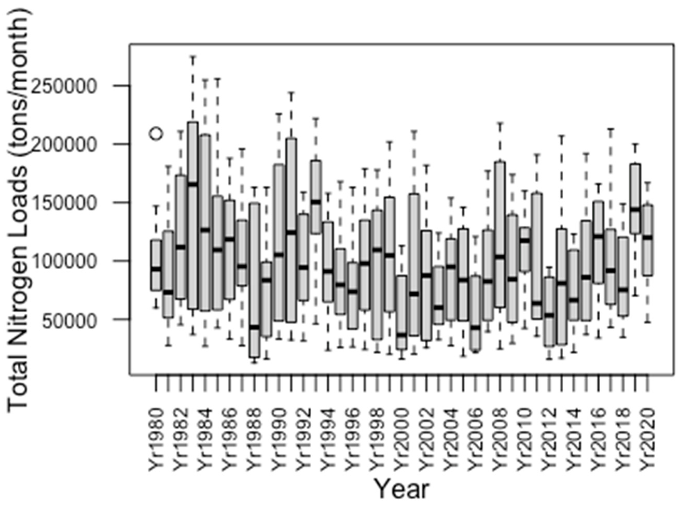
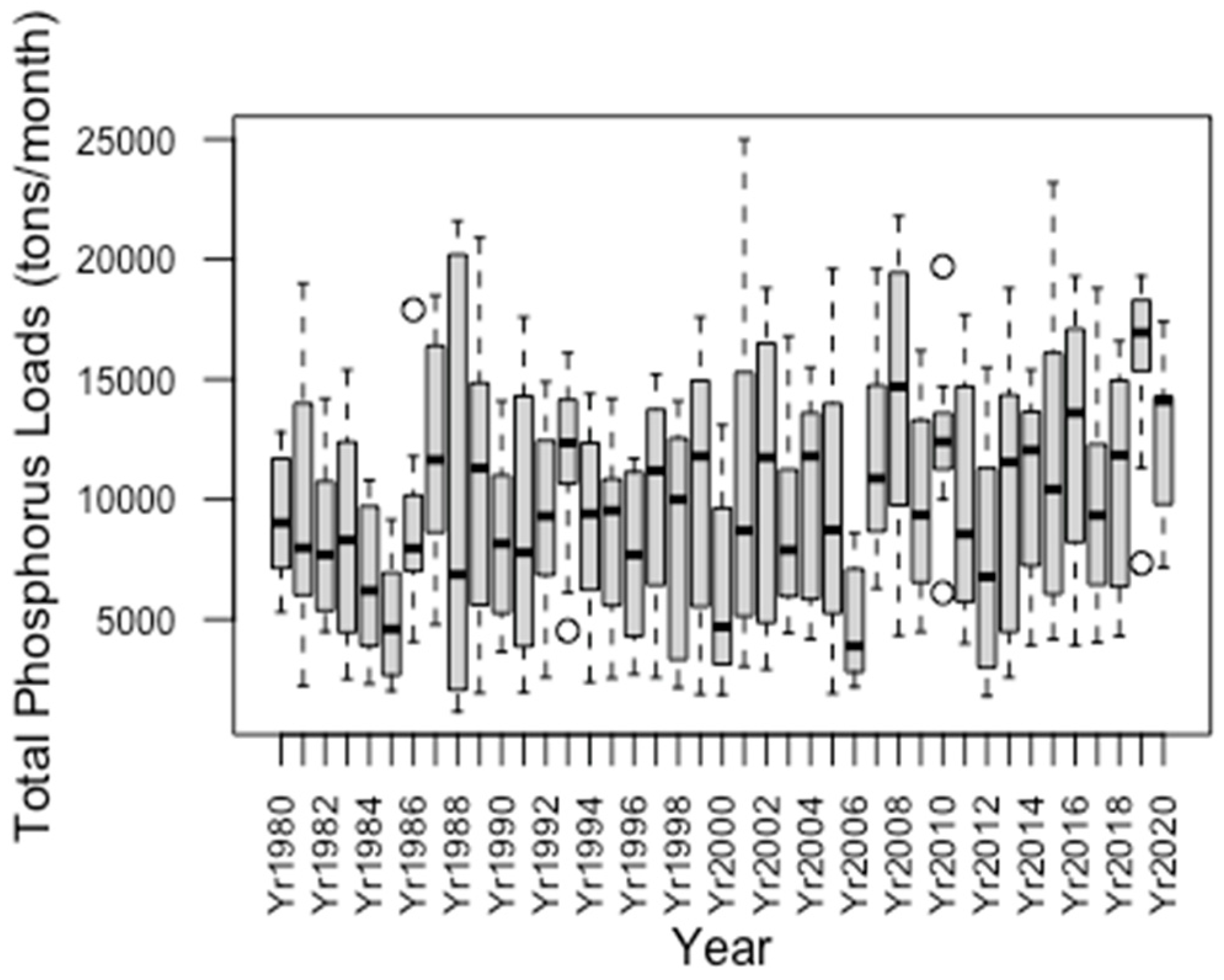
The mean monthly TN and TP loads at USGS monitoring station 07373420 from 1980 to 2020 are shown in Figure 3 and Figure 4, respectively. Figure 3 shows that the mean of the monthly TN loads from 1980 to 2020 observed at Station 07373420 was 99,323.61 ± 23,683.35 tons/month with a range of 54,308.33 to 153,916.67 tons/month. The mean monthly TN loads slightly decreased from 109037.50 tons/month in the 1980s to 105,543.33 tons/month in the 1990s, significantly declined to 83,910.83 tons/month in the 2000s, and then slightly increased to 98,472.73 tons/month in the 2010s. The maximum TN loads occurred in the 1980s and decreased in the last three decades. From Figure 4, it can be seen that the mean of monthly TP loads from 1980 to 2020 observed at Station 07373420 was 9830.77 ± 2217.51 tons/month with a range of 4791.67 to 16,003.33 tons/month. The mean monthly TP loads increased from 8869.00 tons/month in the 1980s to 9263.42 tons/month in the 1990s, and slightly continuously increased to 9749.67 tons/month in the 2000s, and then significantly increased to 11,294.62 tons/month in the 2010s. The mean monthly TP loads peaked in the 2010s, showing a persistent increasing trend.

3.2. Seasonal Variations

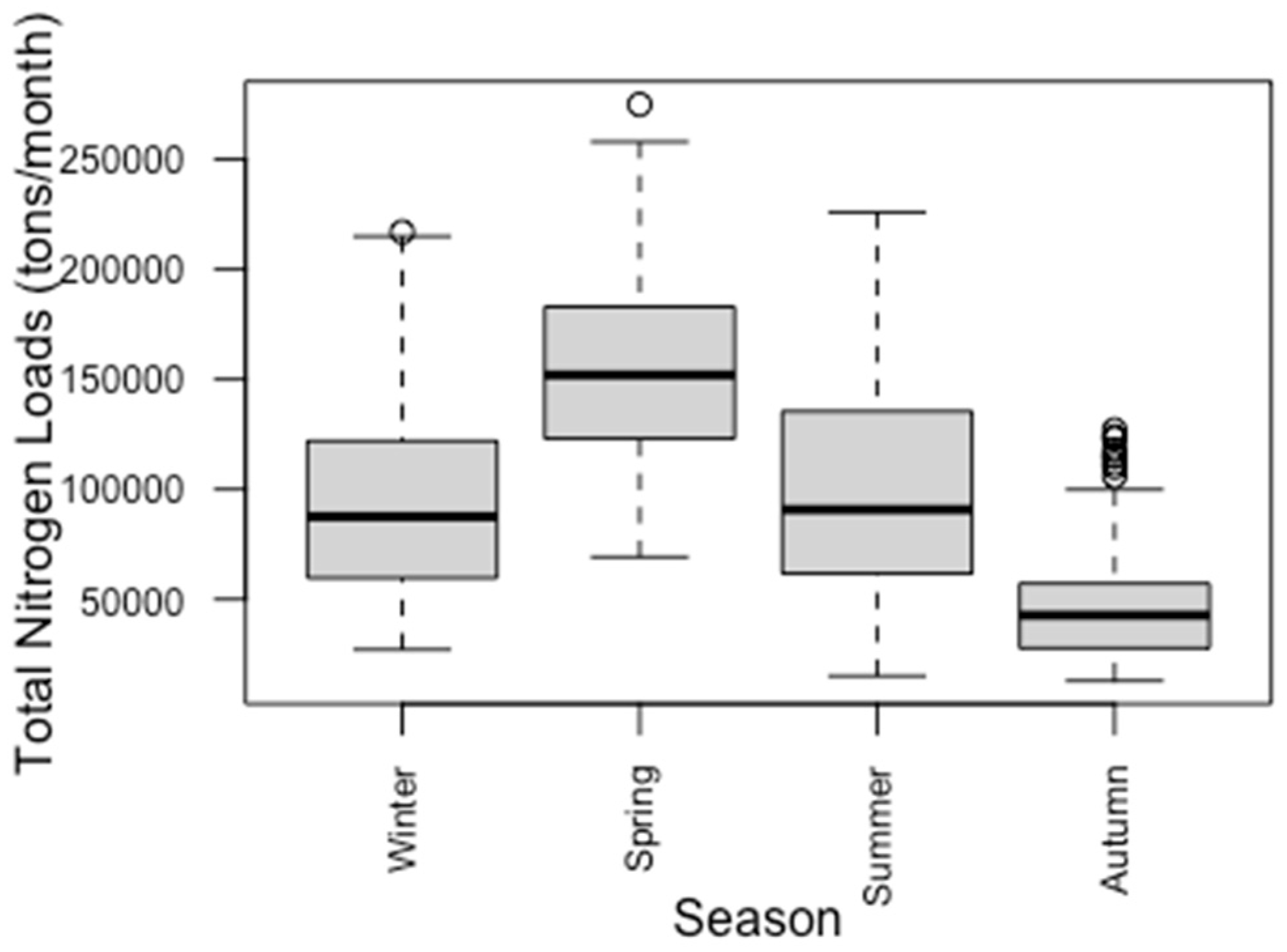
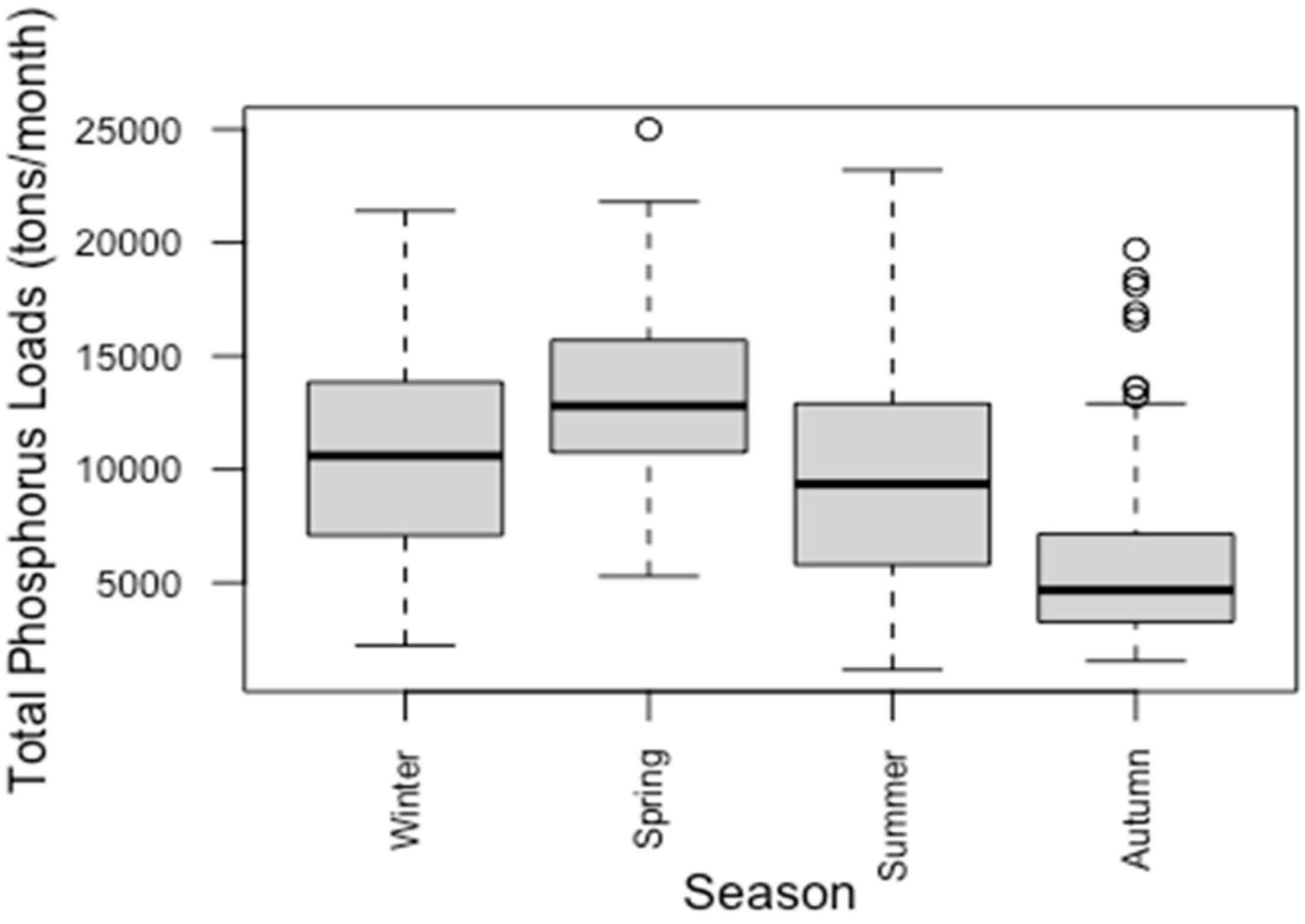
The seasonal variations in the mean monthly TN and TP loads at Station 07373420 are presented in Figure 5 and Figure 6, respectively. These figures suggest that the mean monthly nutrient loads in autumn were lowest while those in spring were highest. In addition, the mean monthly TP load was maximum in spring and lowest in autumn (spring > winter > summer > autumn) while the mean monthly TN loads in summer was slightly higher than that in winter. Similar to TP loads, TN loads in spring are consistently larger than those in the other three seasons. A relatively high mean in monthly TN loads (154,659.35 tons) was observed in spring, followed by summer (99,542.28 tons), winter (94,913.82 tons), and autumn (47,773.98 tons), while the highest mean monthly TP loads were in spring (13,273.90 tons), followed by winter (10,680.24 tons), summer (9472.11 tons), and autumn (5896.83 tons). The mean monthly TN and TP loads for different seasons at Station 07373420 were computed using the data from 1980 to 2020, sorting by springs, summers, autumns, and winters. The contributions of different seasons’ nutrient loads to the total nutrient loads varied considerably. TN nutrient loads in spring contribute the largest proportion (39%), followed by summer (25%), winter (24%), and autumn (12%), while seasonal contribution of TP loads was in the order: spring (34%), winter (27%), summer (24%), and autumn (15%).

3.3. Nutrient Loads Prediction

3.3.1. ARIMA Prediction

An autoregressive integrated moving average (ARIMA) model was constructed for the TN and TP nutrient load forecasts. For the monthly TN loads, the augmented Dickey–Fuller test detected stationarity in the dataset (p = 0.01). Therefore, the ARIMA model is suitable for TN loads. ARIMA (1,0,0) × (0,1,1)12 is selected as the final predictive model of TN loads which is expressed as follows:
( 1 ϕ 1 B ) ( 1 B S ) ( X t μ ) = ( 1 + θ 1 S B 1 , S ) w t
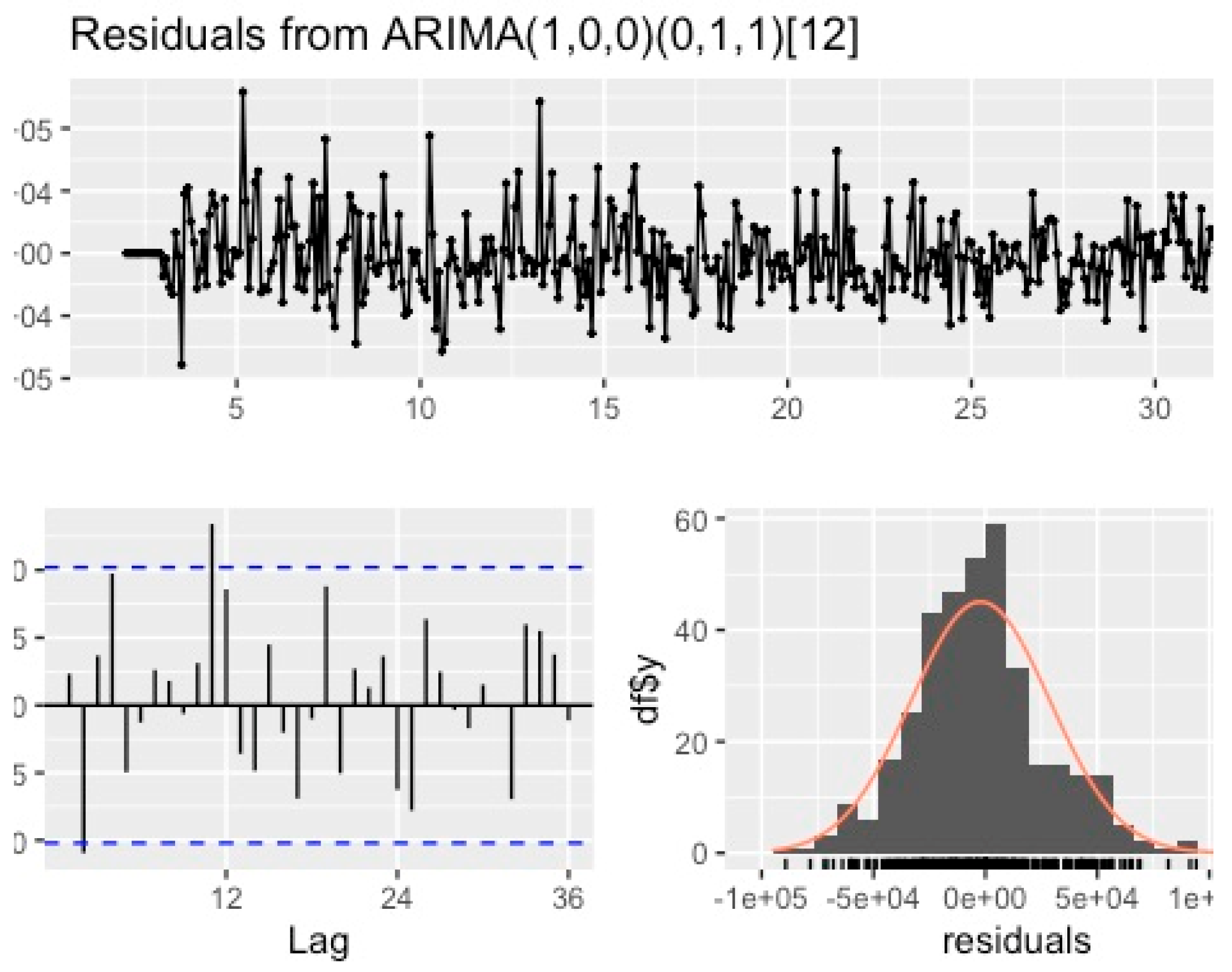
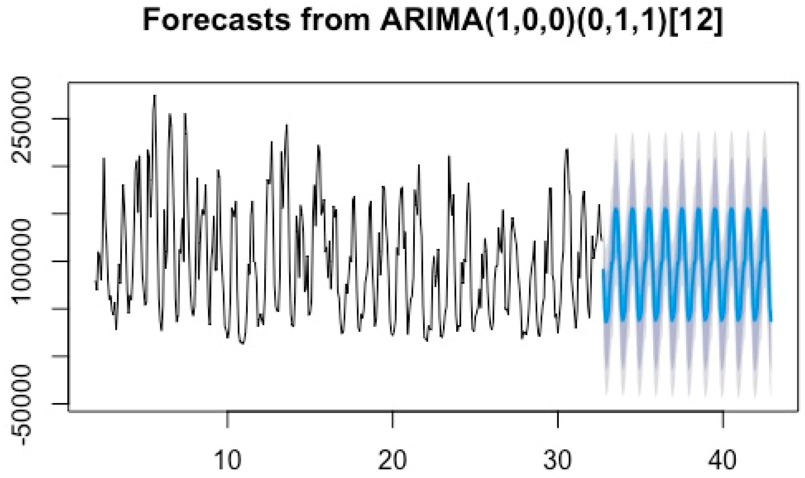
where B is backshift operator, B S is seasonal backshift operator, ϕ 1 = 0.6486 is the coefficient of AR (1) term, and θ 1 S = −0.9261 is the coefficient of seasonal MA (1) term. The coefficients are all highly significant (p < 0.0001). The residuals of ARIMA (1,0,0) × (0,1,1)12 for TN loads are shown in Figure 7. The Durbin–Watson statistic of 1.5373 and the residuals plot indicate that the multi-criteria-based model captures the time series attributes of the observations. The monthly TN forecasting load is shown in Figure 8 along with the observations in the testing dataset.
For TP loads, the augmented Dickey–Fuller Test confirms the stationarity of the dataset (p = 0.01). The final model is defined as ARIMA (1,0,0) × (5,1,0)12,
( 1 ϕ 1 B ) ( 1 ϕ 1 S B 1 , S . . . ϕ 5 S B 5 , S ( 1 B S ) ( X t μ ) = w t
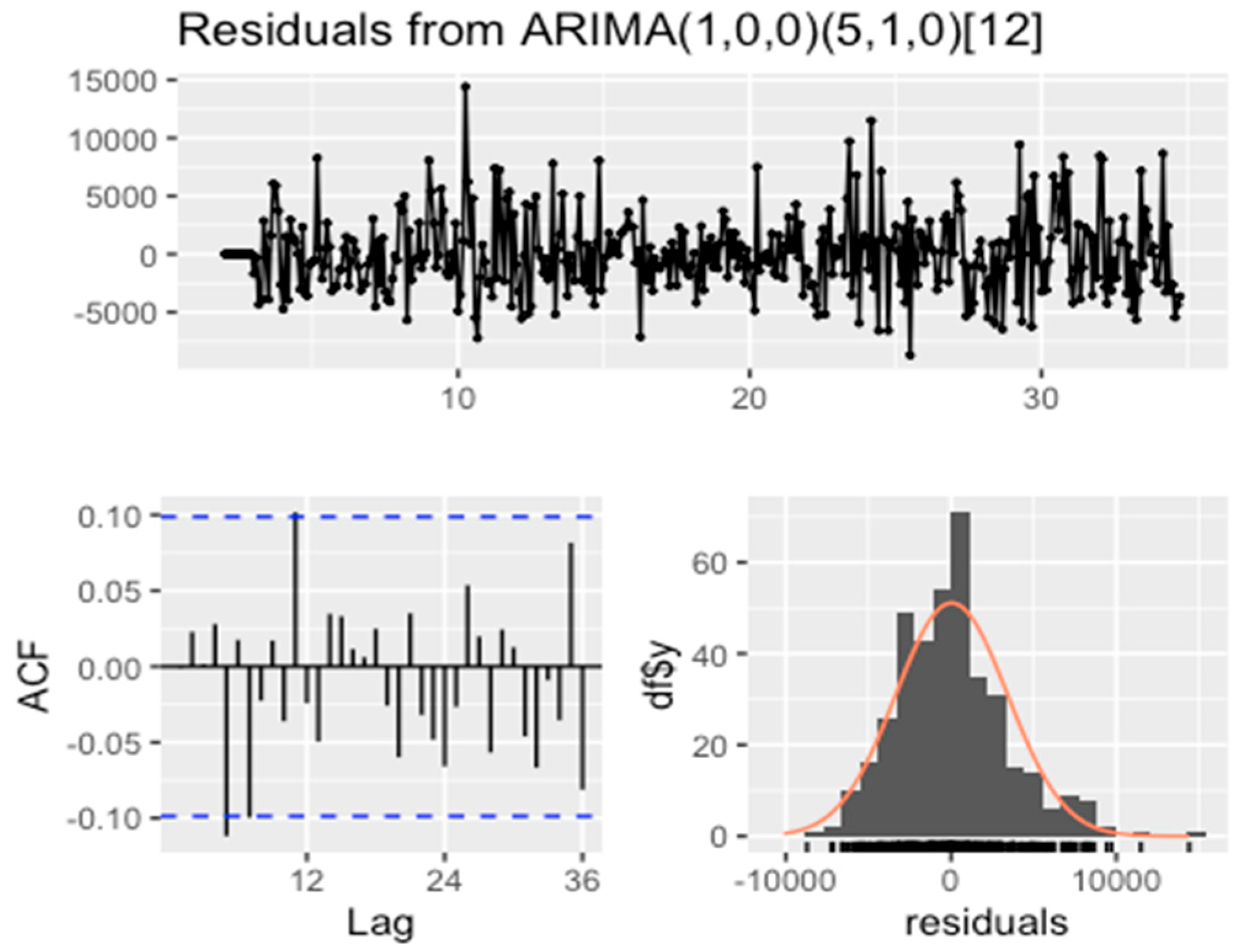
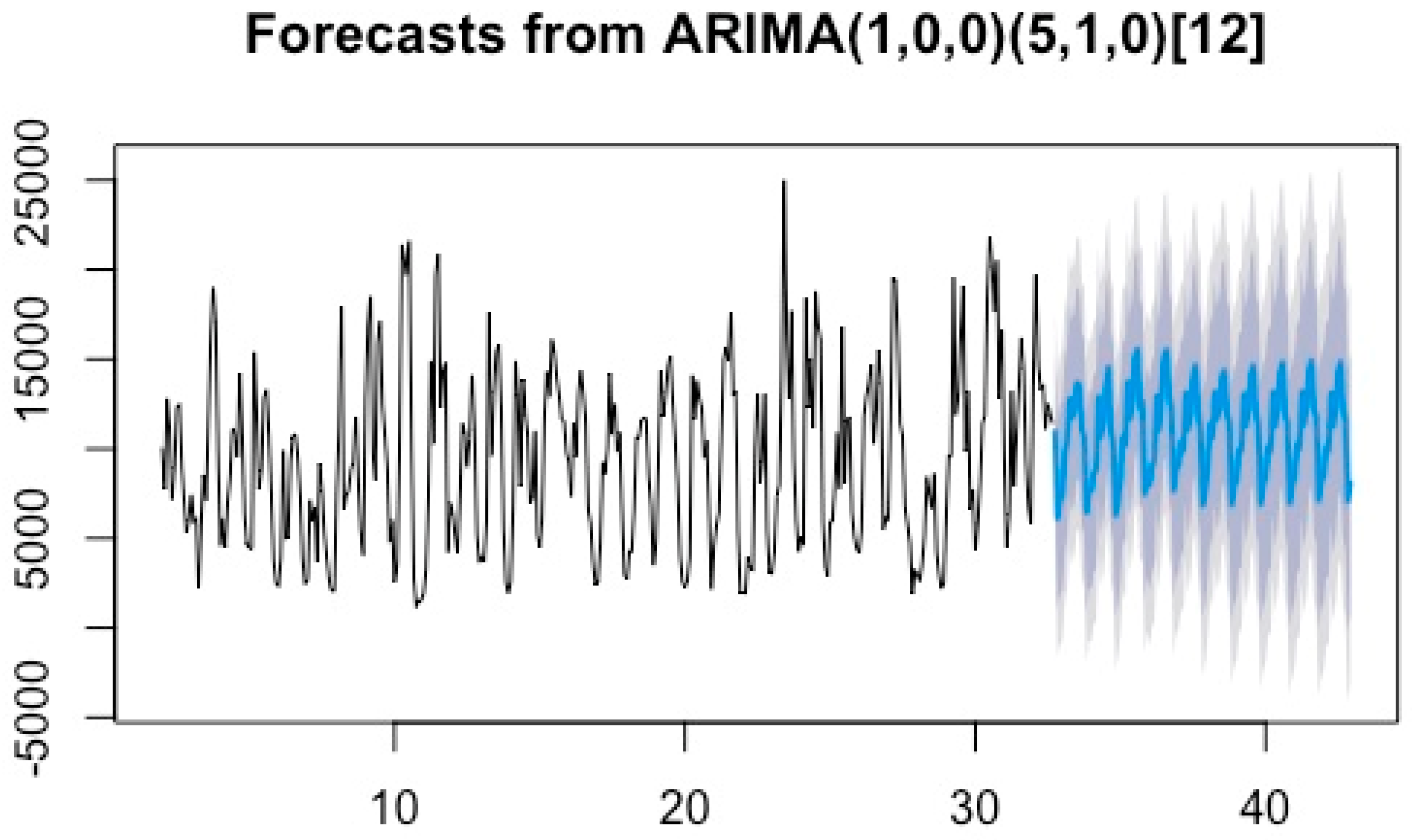
where B is backshift operator, B S is seasonal backshift operator, ϕ 1 = 0.5803 is the highly significant coefficient of AR (1) (p < 0.0001), and ϕ 1 S = −0.7636 (p < 0.0001), ϕ 2 S = −0.6014 (p < 0.0001), ϕ 3 S = −0.3649 (p < 0.0001), ϕ 4 S = −0.3152 (p < 0.0001), and ϕ 5 S = −0.1508 (p < 0.001) are the coefficients of the seasonal AR(1), AR(2), AR(3), AR(4), and AR(5) terms, respectively. The residuals of ARIMA (1,0,0) × (5,1,0)12 are shown in Figure 8. From Figure 9, it can be seen that the model captured the characteristics of the time series observations of the monthly TP loads. The conclusion of non-correlated residuals is supported by the Durbin–Watson statistic of 1.7801, which falls between 1.5 and 2.5. The forecasting values of loads are presented along with original observations in the testing dataset in Figure 10.

3.3.2. GPR Prediction

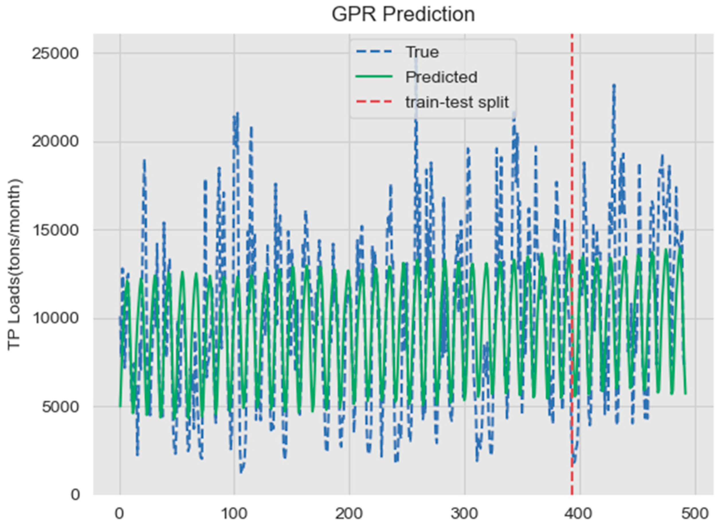
The final optimal GPR model is selected by exploring all kernel functions available. The best combination of hyper parameters and kernel functions for the predictive models of TN and TP loads are selected by the lowest RMSE score. To reach its best forecasting performance, the kernel chosen is a combination of the linear kernel, radial basis function kernel, and exponential sine squared kernel. The optimal set of hyper parameters (the variance and length scale) is determined using cross-validation. The predictions of TN and TP loads from the optimal GPR model are shown in Figure 11 and Figure 12, respectively.

3.3.3. MLP Prediction

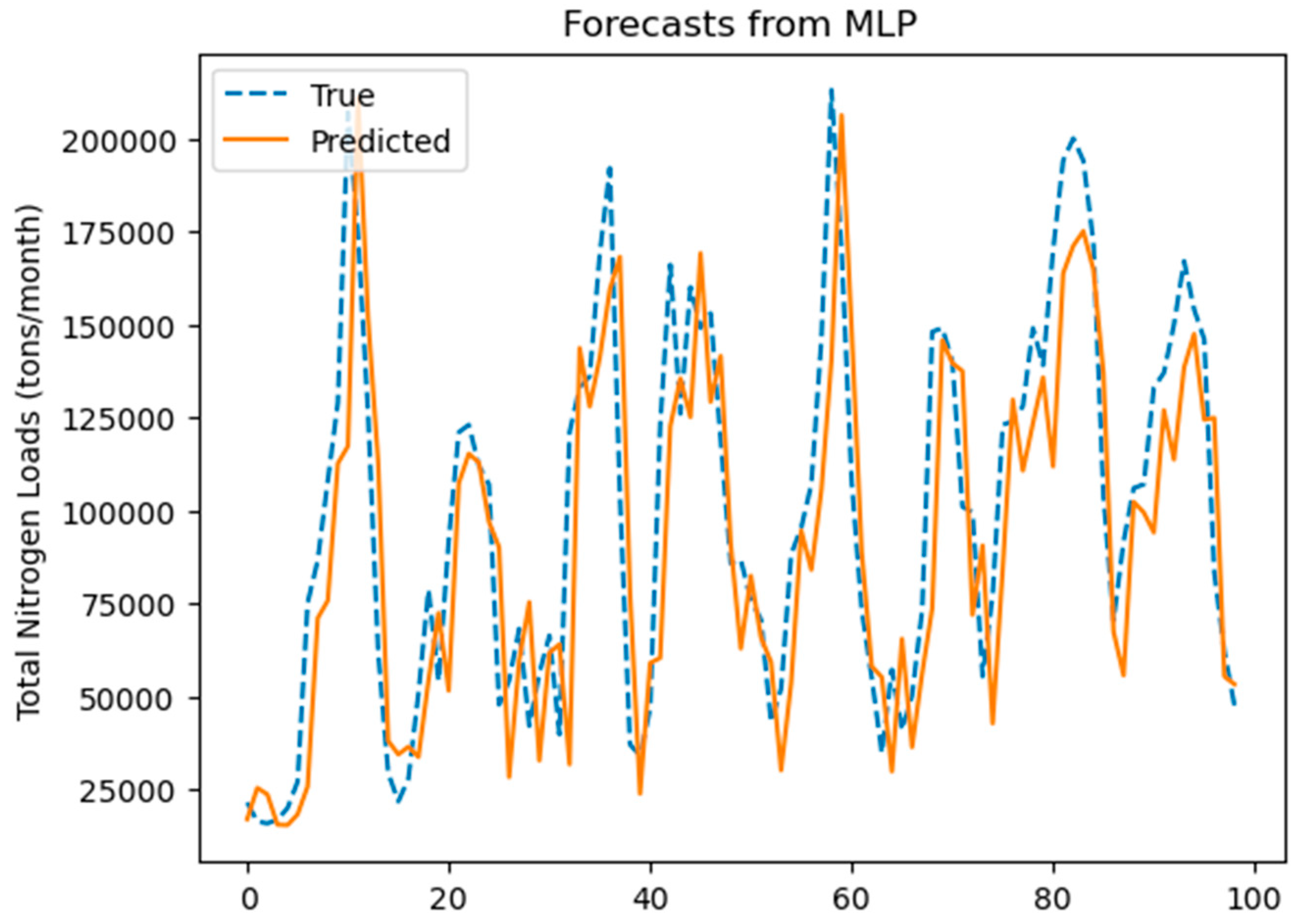
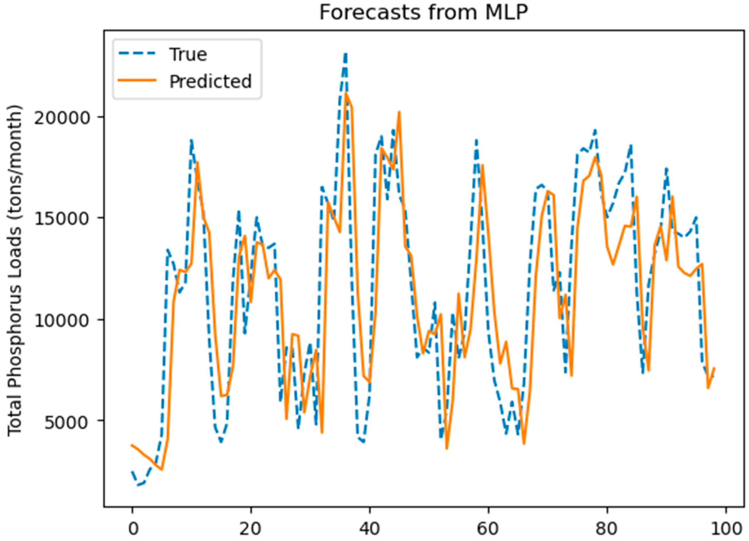
Table 1 presents the best hyperparameters for all six single layer MLP models to predict TN loads. Table 1 suggests that the model with 50 neurons outperforms the others in the RMSE of test dataset, while all six models present a similar R, as shown in Table 1. Thus, a single layer MLP model with 50 neurons may be considered as the most likely best model to forecast TN loads. For the predictive model of TP loads, Table 2 suggests that the model with 200 neurons and the lowest RMSE can be considered as the winner among the other candidates. From Table 1, it can be seen that RMSE decreases over the range of neurons from 10 to 50, then increases from 100 to 150, and then slightly decreases from 150 to 200. Table 2 shows the steady decrease of the RMSE from 10 to 200. All Durbin–Watson statistics ranging between 1.5 and 2.5 indicate that there is no significant presence of autocorrelations in the residuals of models. Figure 13 and Figure 14 represent the original TN and TP loads together with predictions obtained from the reproductions with the lowest RMSE score of the best single layer MLP model, respectively. In Figure 13 and Figure 14, the dotted curve represents the actual values, whereas the solid curves represent the predictions in the test data. It can be seen that the prediction curves of over the test dataset almost match with the curve of the actual observations of TN and TP loads. This implies that the optimal MLP model can learn nonlinear variations of the TN and TP loads quite well.

3.3.4. LSTM Prediction

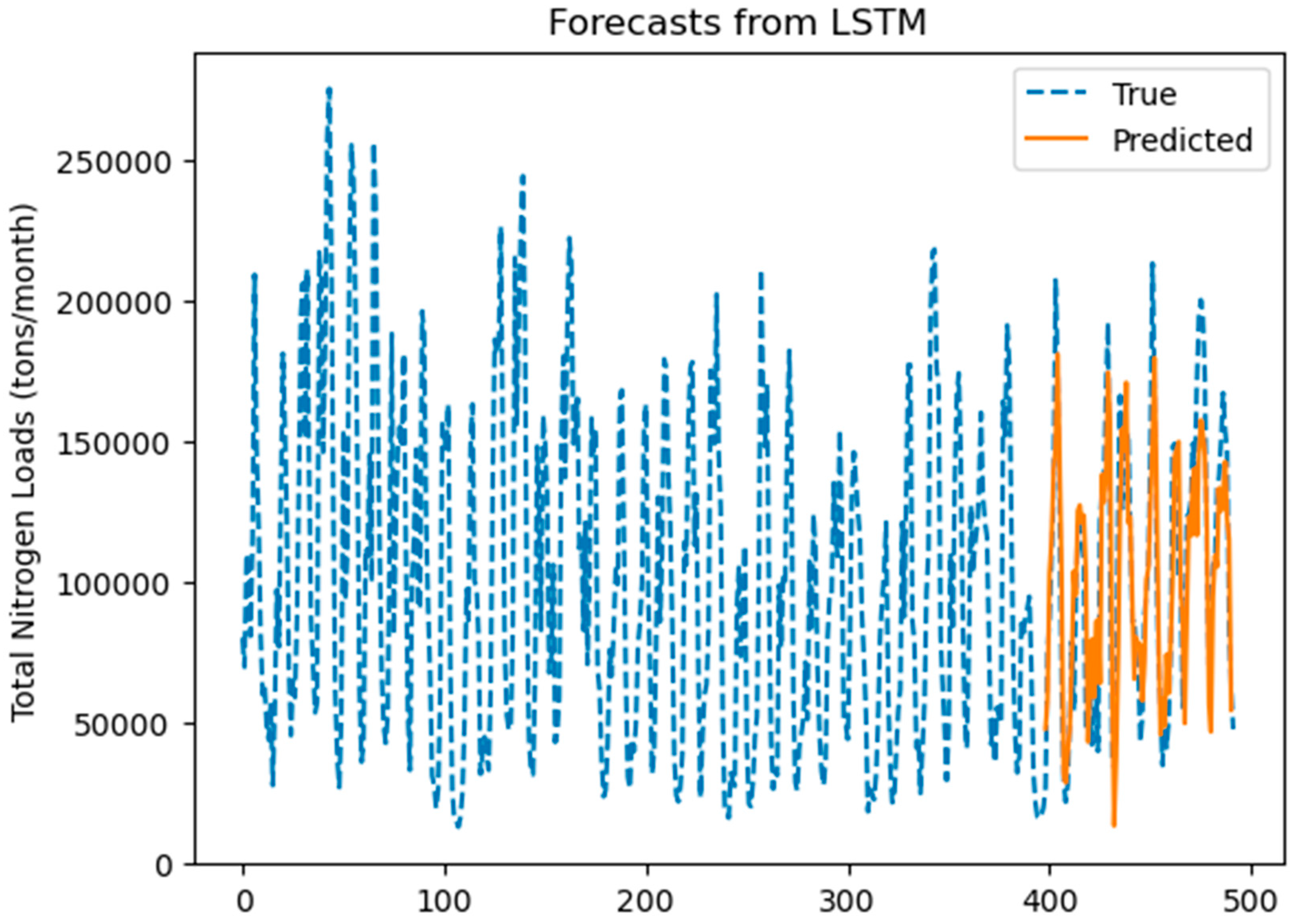
Table 3 presented the best hyperparameters for all six single layer LSTM models to predict TN loads. The results indicate that the model with 100 neurons outperforms in RMSE while all six models present a similar R score. Thus, a single layer LSTM model with 100 neurons may be considered as the most likely best model to forecast TN loads. For the predictive model of TP loads, Table 4 suggests that the model with 30 neurons and the lowest RMSE can be considered as the winner among the other candidates. From Table 3, it can be seen that RMSE decreases over neurons ranging from 10 to 100, and then rises from 100 to 200. Table 4 shows a decrease of the RMSE from 10 to 30 neurons, which then stays around 3730 from 30 to 200. The Durbin–Watson statistics of all models fall between 1.5 and 2.5 and indicate that there is no significant autocorrelation detected in the residuals. Figure 15 and Figure 16 represent the original TN and TP loads together with predicted values obtained from the reproductions of the optimal single-layered LSTM with the lowest test RMSE score, respectively. In Figure 15 and Figure 16, the dotted curve represents the actual observations, whereas the solid curves represent the predictions in the test data. It can be seen that the predictions of the TN and TP loads in the test data closely follow the variations of the true observations. This indicates that the LSTM model is capable of capturing nonlinear patterns in the variations of the nutrient loads.

3.3.5. Evaluation of Model Performance

The best model performance of multi-criteria-based ARIMA, GPR, MLP, and LSTM models of TN and TP loads are summarized in Table 5 and Table 6, respectively. The results show that LSTM persistently outperformed in the predictions of TN loads while MLP slightly outperformed LSTM in the forecasts of TP loads. In addition, although GPR has a better test RMSE score, its R score is much lower than ARIMA. Moreover, ARIMA achieved the best R score compared to the other three models. Overall, MLP and LSTM persistently outperform GPR and ARIMA due to their ability to capture nonlinearities and complexities in the variations of nutrient loads. Furthermore, the optimal number of input observations in the predictive MLP and LSTM models of TP loads are consistent with that of autoregressive order in ARIMA. It is worth highlighting that the multi-criteria-based ARIMA exhibits competitive performance.

4. Discussion and Conclusions

The decreasing pattern of variations in TN from 1980 to 2020 implies that excessive nutrient fluxes are manageable through collective efforts [3]. Nutrient load forecasting is one of the research focuses in the environmental science community. Precise prediction of nutrient loads, however, is a challenging because of their complex origins and nonlinear behavior. There are several factors that can impact predictions of temporal and spatial properties such as land usage, industrial activities, precipitation, agriculture, and the distribution location of excess nutrients. In this study, ARIMA, GPR, MLP, and LSTM models were developed to predict the nutrient loads at USGS 07373420. MLP and LSTM persistently achieved the best performance compared to the ARIMA and GPR models because the neural network type models are capable of capturing complex underlying processes and nonlinear nature in the variations of nutrient loads. ARIMA, however, demonstrates comparable forecasting ability if it is selected based on multi-criteria, which indicates that AIC value alone is not adequate for selection of the best ARIMA model, while residuals of the fitted model and the significance of the coefficients of model are the most influential factors which affect the accuracy of predictions from ARIMA. In order to select the ARIMA with best performance, multiple selection criteria, including results of the autocorrelation function, the partial autocorrelation function, significance of coefficients, Akaike information criterion values, residuals of the fitted model, and test errors, should be considered. The RMSE scores indicate that ARIMA (1,0,0) × (0,1,1)12 and ARIMA (1,0,0) × (5,1,0)12 are the best models in the prediction of TN loads and TP loads, respectively. By experimenting with a wide range of combinations of hyper parameters, the optimal architecture of the single-layer MLP for TN loads is identified as the model with 50 neurons, while for TP loads, the number of neurons is 200. For single-layered LSTM, the model with best performance has 100 neurons for TN loads and 30 for TP loads. In addition, the optimal number of input observations needed in the predictive MLP and LSTM models of TP loads are consistent with those of autoregressive order in ARIMA. Moreover, although GPR achieved slightly better RMSE score than ARIMA, which demonstrated the power of Bayesian inference in prediction, R-squared scores are much lower than ARIMA. Furthermore, it is found, surprisingly, that the Rmsprop optimizer performed well in the LSTM models to forecast TP loads instead of the robust Adam optimizer. This study demonstrates the combination of several criteria is an effective tool to select the ARIMA with the best performance and explores the ability of machine learning models to accurately reproduce nutrient loads delivered to the Gulf of Mexico. The future plan is to improve the accuracy of predictions by hybridizing models with superior performances and to investigate the characteristics of the predictive models in the upper, middle, and lower Mississippi/Atchafalaya River Basin.

Author Contributions

Study conceptualization, Y.Z., H.F. and S.Y.; data processing and modeling tasks, Y.Z., H.F. and S.Y.; analysis and result interpretation, Y.Z., H.F. and S.Y.; writing—original draft preparation, Y.Z.; writing—review and editing, H.F. and S.Y. All authors have read and agreed to the published version of the manuscript.

Funding

This research received no external funding.

Data Availability Statement

The data are publicly available on the USGS website (https://www.sciencebase.gov/catalog/item/61c08ec5d34ee9cd54ed3425).

Acknowledgments

We gratefully acknowledge the staff members in the Office of Education Programs and the Computational Science Initiative at Brookhaven National Laboratory for their support and assistance in this research. We gratefully acknowledge the three anonymous reviewers for their helpful comments and advice, which have substantially improved the quality of this manuscript. This work was supported in part by the U.S. Department of Energy, Office of Science, Office of Workforce Development for Teachers and Scientists (WDTS) under the Visiting Faculty Program (VFP).

Conflicts of Interest

We declare that we do not have any commercial or associative interest that represents a conflict of interest in connection with the work submitted.

References

  1. Diaz, R.J.; Rosenberg, R. Spreading Dead Zones and Consequences for Marine Ecosystems. Science 2008, 321, 926–929. [Google Scholar] [CrossRef] [PubMed]
  2. U.S. Environmental Protection Agency (USEPA). Nutrient Criteria Technical Guidance Manual—Lakes and Reservoirs; U.S. Environmental Protection Agency, Office of Water: Washington, DC, USA, 2000; 232p.
  3. Robertson, D.M.; Schwarz, G.E.; Saad, D.A.; Alexander, R.A. Incorporating Uncertainty into the Ranking of SPARROW Model Nutrient Yields from Mississippi/Atchafalaya River Basin Watersheds. J. Am. Water Resour. Assoc. 2009, 45, 534. [Google Scholar] [CrossRef] [PubMed]
  4. Robertson, D.M.; Saad, D.A. Nitrogen and Phosphorus Sources and Delivery from the Mississippi/Atchafalaya River Basin: An Update Using 2012 SPARROW Models. J. Am. Water Resour. Assoc. 2021, 57, 406. [Google Scholar] [CrossRef]
  5. Nie, J.; Mirza, S.; Viteritto, M.; Li, Y.; Witherell, B.B.; Deng, Y.; Yoo, S.; Feng, H. Estimation of nutrient (N and P) fluxes into Newark Bay, USA. Mar. Pollut. Bull. 2023, 190, 114832. [Google Scholar] [CrossRef]
  6. He, S.; Chu, T.-J.; Lu, Z.; Li, D. Coupling Imports of Dissolved Inorganic Nitrogen and Particulate Organic Matter by Aquaculture Sewage to Zhangjiang Estuary, Southeastern China. Water 2024, 16, 2054. [Google Scholar] [CrossRef]
  7. Morales-Marín, L.A.; Chun, K.P.; Wheater, H.S.; Lindenschmidt, K.E. Trend analysis of nutrient loadings in a large prairie catchment. Hydrol. Sci. J. 2017, 62, 657. [Google Scholar] [CrossRef]
  8. Feng, H.; Qian, Y.; Cochran, J.K.; Zhu, Q.; Hu, W.; Yan, H.; Li, L.; Huang, X.; Chu, Y.S.; Liu, H.; et al. Nanoscale measurement of trace element distributions in Spartina alterniflora root tissue during dormancy. Sci. Rep. 2017, 7, 40420. [Google Scholar] [CrossRef]
  9. Antonopoulos, V.Z.; Papamichail, D.M.; Mitsiou, K.A. Statistical and trend analysis of water quality and quantity data for the Strymon River in Greece. Hydrol. Earth Syst. Sci. 2001, 5, 679. [Google Scholar] [CrossRef]
  10. Alexander, R.B.; Smith, R.A. Trends in the nutrient enrichment of U.S. rivers during the late 20th century and their relation to changes in probable stream trophic conditions. Limnol. Oceanogr. 2006, 51, 639. [Google Scholar] [CrossRef]
  11. Fernández del Castillo, A.; Yebra-Montes, C.; Verduzco Garibay, M.; de Anda, J.; Garcia-Gonzalez, A.; Gradilla-Hernández, M.S. Simple Prediction of an Ecosystem-Specifific Water Quality Index and the Water Quality Classifification of a Highly Polluted River through Supervised Machine Learning. Water 2022, 14, 1235. [Google Scholar] [CrossRef]
  12. Du, J.L.; Feng, H.; Nie, J.; Li, Y.; Witherell, B.B. Characterisation and assessment of spatiotemporal variations in nutrient concentrations and fluxes in an urban watershed: Passaic River Basin, New Jersey, USA. Int. J. Environ. Pollut. 2018, 63, 154. [Google Scholar] [CrossRef]
  13. LIoyd, C.E.M.; Freer, J.E.; Johnes, P.J.; Collins, A.L. Using hysteresis analysis of high-resolution water quality monitoring data, including uncertainty, to infer controls on nutrient and sediment transfer in catchments. Sci. Total Environ. 2016, 543, 388. [Google Scholar] [CrossRef]
  14. Goolsby, D.A.; Battaglin, W.A.; Lawrence, G.B.; Artz, R.S.; Aulenbach, B.T.; Hooper, R.P.; Keeney, D.R.; Stensland, G.J. Flux and Sources of Nutrients in the Mississippi-Atchafalaya River Basin: Topic 3 Report for the Integrated Assessment on Hypoxia in the Gulf of Mexico; NOAA Coastal Ocean Program Decision Analysis Series No. 17; NOAA Coastal Ocean Program: Silver Spring, MD, USA, 1999; 130p. [Google Scholar]
  15. David, M.B.; Drinkwater, L.E.; McIssac, G.F. Sources of Nitrate Yields in the Mississippi River Basin. J. Environ. Qual. 2010, 39, 1657. [Google Scholar] [CrossRef]
  16. Jacobson, L.M.; David, M.B.; Drinkwater, L.E. A Spatial Analysis of Phosphorus in the Mississippi River Basin. J. Environ. Qual. 2011, 40, 931. [Google Scholar] [CrossRef] [PubMed]
  17. Feng, H.; Qian, Y.; Cochran, J.K.; Zhu, Q.; Heilbrun, C.; Li, L.; Hu, W.; Yan, H.; Huang, X.; Ge, M.; et al. Seasonal differences in trace element concentrations and distribution in Spartina alterniflora root tissue. Chemosphere 2018, 204, 359. [Google Scholar] [CrossRef] [PubMed]
  18. Schreiber, S.G.; Schreiber, S.; Tanna, R.N.; Roberts, D.R.; Arciszewski, T.J. Statistical tools for water quality assessment and monitoring in river ecosystems—A scoping review and recommendations for data analysis. Water Qual. Res. J. 2022, 57, 40. [Google Scholar] [CrossRef]
  19. de Andrade Costa, D.; Soares de Azevedo, J.P.; dos Santos, M.A.; dos Santos, R. Water quality assessment based on multivariate statistics and water quality index of a strategic river in the Brazilian Atlantic Forest. Sci. Rep. 2020, 10, 22038. [Google Scholar] [CrossRef]
  20. Yang, W.; Zhao, Y.; Wang, D.; Wu, H.; Lin, A.; He, L. Using Principal Components Analysis and IDW Interpolation to Determine Spatial and Temporal Changes of Surface Water Quality of Xin’anjiang River in Huangshan, China. Int. J. Environ. Res. Public Health 2020, 17, 2942. [Google Scholar] [CrossRef] [PubMed] [PubMed Central]
  21. Singh, K.P.; Malik, A.; Mohan, D.; Sinha, S. Multivariate statistical techniques for the evaluation of spatial and temporal variations in water quality of Gomti River (India)—A case study. Water Res. 2004, 38, 3980. [Google Scholar] [CrossRef]
  22. Dutta, S.; Dwivedi, A.; SureshKumar, M. Use of water quality index and multivariate statistical techniques for the assessment of spatial variations in water quality of a small river. Environ. Monit. Assess. 2018, 190, 718. [Google Scholar] [CrossRef]
  23. Zhen, Y.; Feng, H.; Yoo, S. Structuring Nutrient Yields throughout Mississippi/Atchafalaya River Basin Using Machine Learning Approaches. Environments 2023, 10, 162. [Google Scholar] [CrossRef]
  24. Neitsch, S.L.; Arnold, J.G.; Kiniry, J.R.; Williams, J.R. Soil and Water Assessment Tool Theoretical Documentation Version 2009; Texas Water Resources Institute: College Station, TX, USA, 2011. [Google Scholar]
  25. Worku, T.; Khare, D.; Tripathi, S. Modeling runoff–sediment response to land use/land cover changes using integrated GIS and SWAT model in the Beressa watershed. Environ. Earth Sci. 2017, 76, 550. [Google Scholar] [CrossRef]
  26. Robertson, D.M.; Saad, D.A. SPARROW Models Used to Understand Nutrient Sources in the Mississippi/Atchafalaya River Basin. J. Environ. Qual. 2013, 42, 1422. [Google Scholar] [CrossRef]
  27. Robertson, D.M.; Saad, D.A.; Schwarz, G.E. Spatial Variability in Nutrient Transport by HUC8, State, and Subbasin based on Mississippi/Atchafalaya River Basin SPARROW models. J. Am. Water Resour. Assoc. 2014, 50, 988. [Google Scholar] [CrossRef]
  28. Adebiyi, A.A.; Adewumi, A.O.; Ayo, C.K. Stock Price Prediction Using the ARIMA Model. In Proceedings of the UKSim-AMSS 16th International Conference on Computer Modeling and Simulation, Cambridge, UK, 26–28 March 2014. [Google Scholar]
  29. Alonso, A.M.; Garcia-Martos, C. Time Series Analysis—Forecasting with ARIMA Models; Universidad Carlos III de Madrid: Madrid, Spain; Universidad Politecnica de Madrid: Madrid, Spain, 2012. [Google Scholar]
  30. Brownlee, J. Time Series Prediction with LSTM Recurrent Neural Networks in Python with Keras. 2016. Available online: https://machinelearningmastery.com/time-series-prediction-lstm-recurrent-neural-networks-python-keras/ (accessed on 20 May 2019).
  31. Box, G.; Jenkins, G. Time Series Analysis: Forecasting and Control; Holden-Day: San Francisco, CA, USA, 1970. [Google Scholar]
  32. Earnest, A.; Chen, M.I.; Ng, D.; Sin, L.Y. Using Autoregressive Integrated Moving Average (ARIMA) Models to Predict and Monitor the Number of Beds Occupied During a SARS Outbreak in a Tertiary Hospital in Singapore. BMC Health Serv. Res. 2005, 5, 36. [Google Scholar] [CrossRef] [PubMed]
  33. Krauss, C.; Do, X.A.; Huck, N. Deep neural networks, gradient- boosted trees, random forests: Statistical arbitrage on the S&P 500. Eur. J. Oper. Res. 2017, 259, 689. [Google Scholar] [CrossRef]
  34. Patterson, J.; Gibson, A. Deep Learning: A Practitioner’s Approach; O’Reilly Media: Sevastopol, CA, USA, 2017; ISBN 10 1491914254/13: 978-1491914250. [Google Scholar]
  35. Bhandari, H.N.; Rimal, B.; Pokhrel, N.R.; Rimal, R.; Dahal, K.R.; Khatri, R.K.C. Predicting stock market index using LSTM. Mach. Learn. Appl. 2022, 9, 100320. [Google Scholar] [CrossRef]
  36. Hochreiter, S. The vanishing gradient problem during learning recurrent neural nets and problem solutions. Int. J. Uncertain. Fuzziness Knowl.-Based Syst. 1998, 6, 107. [Google Scholar] [CrossRef]
  37. Rasmussen, C.E.; Williams, C.K.I. Gaussian Processes for Machine Learning; MIT Press: Cambridge, MA, USA, 2006; ISBN 978-0-262-18253-9. [Google Scholar]
  38. Haykin, S. Neural Networks: A Comprehensive Foundation; Prentice Hall PTR: Lebanon, IN, USA, 1994. [Google Scholar]
  39. Elman, J.L. Finding structure in time. Cogn. Sci. 1990, 14, 179. [Google Scholar] [CrossRef]
  40. Hochreiter, S.; Schmidhuber, J. Long short-term memory. Neural Comput. 1997, 9, 1735. [Google Scholar] [CrossRef]
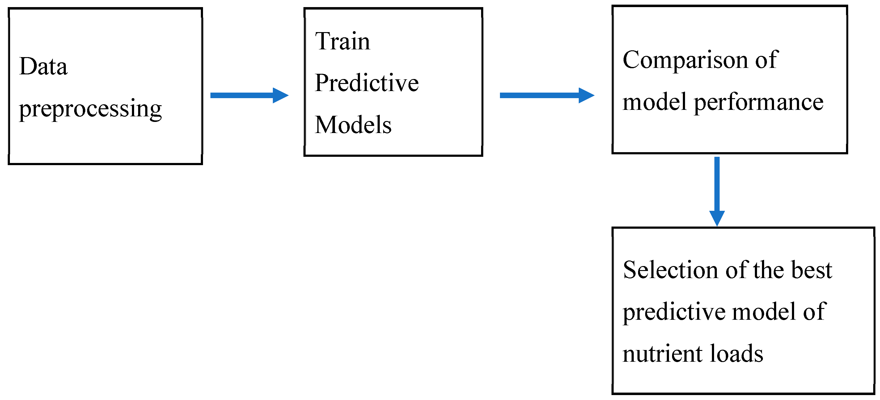
Figure 1. Schematic diagram of methodology.
Water 16 02857 g001
Figure 2. USGS water station 07373420 (STFR) concerned in Mississippi/Atchafalaya River Basin indicated by yellow placeholder.
Water 16 02857 g002
Figure 3. Mean monthly TN loads from 1980 to 2020.
Water 16 02857 g003
Figure 4. Mean monthly TP loads from 1980 to 2020.
Water 16 02857 g004
Figure 5. Seasonal mean monthly total nitrogen from 1980 to 2020.
Water 16 02857 g005
Figure 6. Seasonal mean monthly total phosphorus from 1980 to 2020.
Water 16 02857 g006
Figure 7. The residuals of ARIMA (1,0,0) × (0,1,1)12 for TN loads.
Water 16 02857 g007
Figure 8. The predictions from ARIMA (1,0,0) × (0,1,1)12 for TN loads. The blue line represents the predictions of TN loads and the grey line represents the actual observations.
Water 16 02857 g008
Figure 9. The residuals of ARIMA (1,0,0) × (5,1,0)12 for TP loads.
Water 16 02857 g009
Figure 10. The forecasts of TP loads from ARIMA (1,0,0) × (5,1,0)12. The blue solid line represents the predictions of TP loads.
Water 16 02857 g010
Figure 11. The predictions from the best single layer GPR for TN loads.
Water 16 02857 g011
Figure 12. The predictions from the best single layer GPR for TP loads.
Water 16 02857 g012
Figure 13. The predictions from best single layer MLP (optimizer: Adam; neurons: 50; learning rate: 0.01; inputs: 5; epochs: 50; batch size: 1) for TN loads.
Water 16 02857 g013
Figure 14. The predictions from the best single layer MLP (optimizer: Nadam; neurons: 200; learning rate: 0.01; inputs: 6; epochs: 50; batch size: 8) for TP loads.
Water 16 02857 g014
Figure 15. The predictions from the optimal LSTM with a single hidden layer (optimizer: Adam; neurons: 100; learning rate (default): 0.01; inputs: 4; epochs: 100; batch size: 8) for TN loads in the test dataset.
Water 16 02857 g015
Figure 16. The predictions from the best single layer LSTM (optimizer: Nadam; neurons: 30; learning rate: 0.01; inputs: 2; epochs: 100; batch size: 1) for TP loads in the test dataset.
Water 16 02857 g016
Table 1. List of the best hyper parameters for the single-layer MLP model for predictions of TN loads.
No. of NeuronsOptimizerNo. of EpochsBatch SizeNo. of InputsAverage Test RMSEAverage R ScoreThe Durbin–Watson Statistic of Residuals
10Rmsprop501629,779.760.6561.7493
30Nadam501529,690.460.6441.6609
50Adam501529,454.620.6611.8440
100Nadam501529,463.610.6611.8209
150Adam1501231,195.690.6191.7408
200Adam501229,614.520.6201.7352
Table 2. List of the best hyper parameters for single layer MLP model for predictions of TP loads.
No. of NeuronsOptimizerNo. of EpochsBatch SizeNo. of InputsAverage Test RMSEAverage R ScoreThe Durbin–Watson Statistic of Residuals
10Adam100263692.700.4851.9298
30Adam100153692.940.4771.8508
50Adam100253682.140.4881.8604
100Adam50453661.150.4861.8574
150Adam50253659.850.4921.8736
200Nadam50863645.580.4921.8964
Table 3. List of the best hyper parameters for the single layer LSTM model for predictions of TN loads.
No. of NeuronsOptimizerNo. of EpochsBatch SizeNo. Of InputsAverage Test RMSEAverage R ScoreThe Durbin–Watson Statistic of Residuals
10Nadam1001428,199.360.6851.5490
30Nadam1001427,298.640.7071.5024
50Adam1004427,560.250.7101.7185
100Adam1008427,251.680.7071.6255
150Adam1001428,003.560.6951.6555
200Nadam1001428,015.950.6961.7363
Table 4. List of the best hyper parameters for the single layer LSTM model for predictions of TP loads.
No. of NeuronsOptimizerNo. of EpochsBatch SizeNo. of InputsAverage Test RMSEAverage R ScoreThe Durbin–Watson Statistic of Residuals
10Nadam200423748.940.4841.7189
30Nadam100123684.780.4821.5469
50Rmsprop100153742.030.4821.6803
100Rmsprop150123734.910.4691.8065
150Adam100423704.340.4861.5498
200Rmsprop50113737.010.4791.5694
Table 5. Summarizes the best performances of the predictive models for TN loads.
Model TypeTest RMSE Score R-Squared Score
ARIMA34,710.540.760
MLP29,454.620.661
LSTM27,251.680.707
GPR33,035.130.551
Table 6. Summarizes the best performances of the predictive models for TP loads.
Model TypeTest RMSE Score R-Squared Score
ARIMA4390.630.587
MLP3645.580.492
LSTM3684.780.482
GPR4367.470.136
Disclaimer/Publisher’s Note: The statements, opinions and data contained in all publications are solely those of the individual author(s) and contributor(s) and not of MDPI and/or the editor(s). MDPI and/or the editor(s) disclaim responsibility for any injury to people or property resulting from any ideas, methods, instructions or products referred to in the content.